Abstract

Spin-polarizabilities are predicted by calculating the cross-section difference $\sigma_{3/2}-\sigma_{1/2}$ from available data for the resonance couplings $A_{3/2}$ and $A_{1/2}$ and CGLN amplitudes. The forward spin-polarizabilities are predicted to be $\gamma^{(p)}_{0}=-0.58\pm 0.20$ and $\gamma^{(n)}_{0}=+0.38\pm 0.22$ in units of $10^{-4}$ fm⁴ where the different signs are found to be due to the isospin dependencies of the $E_{0+}$ and the $(M,E)^{(1/2)}_{1+}$ amplitudes. The backward spin-polarizabilities are predicted to be $\gamma^{(p)}_{\pi}=-36.6$ and $\gamma^{(n)}_{\pi}=+58.3$, to be compared with the experimental values $\gamma^{(p)}_{\pi}=-36.4\pm 1.5$ and $\gamma^{(n)}_{\pi}=+58.6\pm 4.0$. Electric $\gamma_{E}$ and magnetic $\gamma_{M}$ spin-polarizabilities are introduced and discussed in terms of the $E1$ and $M1/E2$ components of the photo-absorption cross section of the nucleon.

1 Introduction

Studies of the spin-polarizabilities of the nucleon are a fascinating subject of present and future experimental and theoretical research. In a recent article [1] the forward amplitude for polarized Compton scattering by dispersion integrals has been constructed as a guideline for future experiments to extract the spin-polarizabilities of the nucleon. In this work [1] the spin-polarizabilities and their generalized versions are given in terms of pion photoproduction multipoles as well as measured spin-dependent cross sections. Furthermore, references are given of previous experimental and theoretical work.

The purpose of the present paper is to supplement on the important topic of research addressed in [1] by making use of methods to describe the electromagnetic structure of the nucleon as derived in [2, 3, 4, 5, 6, 7, 8]. This method describes the amplitudes for Compton scattering in terms of partial contributions which each can be attributed to a special one-photon or two-photon excitation mechanism. The method is described in detail in [7] and also some more information is given in the next section. The progress achieved in comparison to previous approaches is based on an isospin decomposition of the CGLN amplitudes described in [7]. This makes it possible to avoid the use of available data in terms of partial reaction channels. Through this method it is possible to take advantage of the very precise parametrizations of CGLN amplitudes of Drechsel et al. [9] which are based on the world data of pion photo- and electroproduction and is updated regularly. Furthermore, a method is developed to calculate total cross sections $\sigma_{T}(\omega)$ and spin-dependent cross-section differences $\sigma_{3/2}(\omega)-\sigma_{1/2}(\omega)$ for the nucleon resonances from the resonance couplings $A_{3/2}$ and $A_{1/2}$ which are collected and updated regularly by the Particle Data Group [10]. These resonance couplings contain the effects of the two-pion channel. Therefore, the use of these resonance couplings avoids the problem of the two-pion channel which occurs when relying on the CGLN amplitudes alone. On the basis of these data it is possible to calculate any nucleon structure quantity which is given by a dispersion integral not only in terms of the total quantity but separately in terms of multipolarity and isospin and in terms of resonant or nonresonant excitations. This means that the method translates one-to-one the world data [9] known from photoexcitation experiments into structure constants like the contributions to the Gerasimov-Drell-Hearn (GDH) integral and the electric and magnetic polarizabilities and the spin-polarizabilities for the forward and backward directions.

In the previous paper [7] this method was applied to those quantities where independent directly measured experimental data are available. In a first place these are the cross-section differences $\sigma_{3/2}(\omega)-\sigma_{1/2}(\omega)$ measured by the GDH Collaboration at MAMI (Mainz) and ELSA (Bonn). Good agreement has been obtained between experimental data and predictions. One remarkable result is that the cross-section difference $\sigma_{3/2}(\omega)-\sigma_{1/2}(\omega)$ measured for the $P_{33}(1232)$ resonance is strongly enhanced by the $E2/M1$ ratio. This enhancement amounts to $26\%$ whereas the corresponding quantity is small for $\sigma_{T}(\omega)$. This interesting finding will be analyzed in more detail in the present paper. Another result obtained in the previous paper [7] was that the predicted GDH integrals for the proton and the neutron are in good agreement with the experimental results obtained at MAMI and ELSA. An investigation has also been carried out for the backward spin-polarizabilities where again good agreement has been obtained with directly measured experimental data. However, no investigation has been carried out for the forward spin-polarizabilities because no directly measured data are available. It is the purpose of the present paper to fill this gap of information as far as the predictions are concerned. Since again this investigation of the forward spin-polarizabilities is based on the world data of CGLN amplitudes and resonance couplings $A_{3/2}$ and $A_{1/2}$ the results are expected to be of good precision.

2 Résumé of dispersion theory

Compton scattering is described by the invariant amplitudes $A_{i}(s,t)$ $(i=1-6)$ which are analytic functions in the two variables $s$ and $t$ and, therefore, may be treated in terms of dispersion relations [11, 12, 13, 14]. The degrees of freedom of the nucleon including the structure of the constituent quarks enter into these invariant amplitudes via a cut on the real axis of the complex $s$-plane and in terms of point like singularities on the positive real axis of the $t$-plane as illustrated in Figure 1. The $s$-channel cut contains the total photo-absorption cross section and through a decomposition in terms of excitation mechanisms the complete electromagnetic structure of the nucleon as seen in one-photon processes.

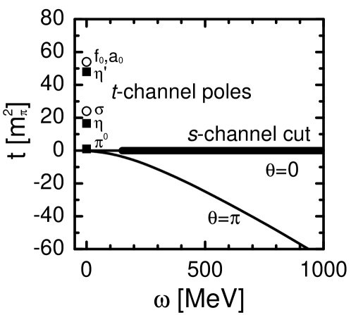
Figure 1: Singularities of the $s$- and the $t$-channel. Horizontal thick line: $s$-channel cut representing the nucleon degrees of freedom, with $\omega$ being the energy of the incoming photon in the lab system. Squares and circles on the vertical real $t$-axis: $t$-channel poles representing the constituent-quark degrees of freedom. The physical range of nucleon Compton scattering extends from the line at $\theta=0$ to the line at $\theta=\pi$.

The point like singularities correspond to the bare masses $m_{0}$ of the mesons which in case of scalar mesons have to be compared with the masses entering into the pole $\sqrt{s_{R}}=M_{R}-\frac{1}{2}\,i\,\Gamma_{R}$ located on the second Riemann sheet of the complex $s$-plane. For the $\sigma$-meson the bare mass is $m_{\sigma}=666$ MeV [8] whereas for the quantities $M_{\sigma}$ and $\Gamma_{\sigma}$ the results $M_{\sigma}=441^{+16}_{-8}$ MeV and $\Gamma_{\sigma}=544^{+18}_{-25}$ [15] have been obtained. Further details may be found in [8]. The relation between the bare mass $m_{0}$ and the pole at $\sqrt{s_{R}}$ can easily be understood from the arguments contained in [16, 17]. Here the propagator is written down in the form

$$P(s)=\frac{1}{m^{2}_{0}+\Pi(s)-s}$$ (1)

where $m_{0}$ is the bare mass of the scalar meson and $\Pi(s)$ a complex analytic function taking into account the effects of decay of the scalar meson into two mesons. The real part of $\Pi(s)$ is equal to the square of the mass shift and the imaginary part proportional to the particle width. The analytic continuation of this propagator has a pole at $s_{R}=(M_{R}-\frac{1}{2}\,i\,\Gamma_{R})^{2}$ on the second Riemann sheet. In case of Compton scattering the reaction $\gamma\gamma\to\sigma\to N\bar{N}$ has to be considered instead of the reaction $\gamma\gamma\to\sigma\to\pi\pi$. This leads to the consequence that $\Pi(s)\equiv 0$, so that the propagator has the form

$$P(s)=\frac{1}{m^{2}_{0}-s},$$ (2)

corresponding to a pole on the positive $t$-axis at $t_{0}=m^{2}_{0}$. Differing from the present procedure, in older works (see [2]) use is made of the pole located on the second Riemann sheet. This is possible by taking into account the reaction $\gamma\gamma\to\sigma\to\pi\pi\to\sigma\to N\bar{N}$ instead of the reaction $\gamma\gamma\to\sigma\to N\bar{N}$. This older procedure is equivalent in principle to the present one but requires a more elaborate numerical calculation.

The point like singularities on the positive real $t$-axis may be related to the structure of the constituent quarks which couple to all mesons with a nonzero meson-quark coupling constant. Of these the $\pi^{0}$- and the $\sigma$-meson are of special interest but also the mesons $\eta$, $\eta^{\prime}$, $f_{0}(980)$ and $a_{0}(980)$ have to be taken into account. In a formal sense the singularities on the positive real $t$-axis correspond to the fusion of two photons with 4-momenta $k_{1}$ and $k_{2}$ and helicities $\lambda_{1}$ and $\lambda_{2}$ to form a $t$-channel intermediate state $|\pi^{0}\rangle$ or $|\sigma\rangle$ or one of the other mesons, from which – in a second step – a proton-antiproton pair is created. In the present case the $N\bar{N}$ pair creation-process is virtual, i.e. the energy is too low to put the proton-antiproton pair on the mass shell (see [2] for more details).

2.1 The kinematics of Compton scattering

In more quantitative terms the content of the forgoing paragraph may be described in the following form. The conservation of energy and momentum in nucleon Compton scattering

$$\gamma(k,\lambda)+N(p)\to\gamma^{\prime}(k^{\prime},\lambda^{\prime})+N^{\prime}(p^{\prime})$$ (3)

is given by

$$k+p=k^{\prime}+p^{\prime}$$ (4)

where $k$ and $k^{\prime}$ are the 4-momenta of the incoming and outgoing photon and $p$ and $p^{\prime}$ the 4-momenta of incoming and outgoing proton. Mandelstam variables are introduced via

$$s=(k+p)^{2}=(k^{\prime}+p^{\prime})^{2},t=(k-k^{\prime})^{2}=(p^{\prime}-p)^{2},u=(k-p^{\prime})^{2}=(k^{\prime}-p)^{2},$$ (5)

$$s+t+u=2m^{2}.$$ (6)

with $m$ being the nucleon mass.

In terms of the Mandelstam variables the scattering angle $\theta$ in the c.m. system is given by

$$\sin^{2}\frac{\theta}{2}=-\frac{st}{(s-m^{2})^{2}}.$$ (7)

The $t$-channel corresponds to the fusion of two photons with four-momenta $k_{1}$ and $k_{2}$ and helicities $\lambda_{1}$ and $\lambda_{2}$ to form a $t$-channel intermediate state $|t\rangle$ from which – in a second step – a proton-antiproton pair is created. The corresponding reaction may be formulated in the form

$$\gamma(k_{1},\lambda_{1})+\gamma(k_{2},\lambda_{2})\to\bar{N}(p_{1})+N(p_{2}).$$ (8)

Since for Compton scattering the related $N\bar{N}$ pair creation-process is virtual, in dispersion theory we have to treat the process described in (8) in the unphysical region. In the c.m. frame of (8) where

$${\bf k_{1}}+{\bf k_{2}}=0$$ (9)

we obtain

$$\sqrt{t}=\sqrt{(k_{1}+k_{2})^{2}}=\omega_{1}+\omega_{2}=W^{t},$$ (10)

where $W^{t}$ is the energy transferred to the $t$-channel via two-photon fusion. At positive $t$ the $t$-channel of Compton scattering $\gamma N\to N\gamma$ coincides with the $s$-channel of the two-photon fusion reaction $\gamma_{1}+\gamma_{2}\to N\bar{N}$.

2.2 Dispersion integrals for the polarizabilities

For the following discussion it is convenient to use the lab frame and to consider special cases for the scattering amplitude $T_{fi}$. These special cases are the extreme forward ($\theta=0$) and extreme backward ($\theta=\pi$) direction where the amplitudes for Compton scattering may be written in the form [18]

$$\frac{1}{8\pi m}[T_{fi}]_{\theta=0}=f_{0}(\omega){\mbox{\boldmath$\epsilon$}}^{\prime}{}^{*}\cdot{\mbox{\boldmath$\epsilon$}}+g_{0}(\omega)\,\mbox{i}\,{\mbox{\boldmath$\sigma$}}\cdot({\mbox{\boldmath$\epsilon$}}^{\prime}{}^{*}\times{\mbox{\boldmath$\epsilon$}}),$$ (11)

$$\frac{1}{8\pi m}[T_{fi}]_{\theta=\pi}=f_{\pi}(\omega){\mbox{\boldmath$\epsilon$}}^{\prime}{}^{*}\cdot{\mbox{\boldmath$\epsilon$}}+g_{\pi}(\omega)\,\mbox{i}\,{\mbox{\boldmath$\sigma$}}\cdot({{\mbox{\boldmath$\epsilon$}}}^{\prime}{}^{*}\times{{\mbox{\boldmath$\epsilon$}}})$$ (12)

with $m$ being the nucleon mass, $\epsilon$ the polarization of the photon and $\sigma$ the spin vector. Equations (11) and (12) can be used to define the polarizabilities and spin-polarizabilities as the lowest-order coefficients in an $\omega$-dependent development of the nucleon-structure dependent parts of the scattering amplitudes:

$$f_{0}(\omega) = -({e^{2}}/{4\pi m})Z^{2}+{\omega}^{2}({\alpha}+{\beta})+{\cal O}({\omega}^{4}),$$ (13)

$$g_{0}(\omega) = \omega\left[-({e^{2}}/{8\pi m^{2}})\,{\kappa}^{2}+{\omega}^{2}{\gamma_{0}}+{\cal O}({\omega}^{4})\right],$$ (14)

$$f_{\pi}(\omega) = \left(1+({\omega^{\prime}\omega}/{m^{2}})\right)^{1/2}[-({e^{2}}/{4\pi m})Z^{2}+\omega\omega^{\prime}({\alpha}-{\beta})+{\cal O}({\omega}^{2}{{\omega}^{\prime}}^{2})],$$ (15)

$$g_{\pi}(\omega) = \sqrt{\omega\omega^{\prime}}[({e^{2}}/{8\pi m^{2}})({\kappa}^{2}+4Z{\kappa}+2Z^{2})+\omega\omega^{\prime}{{\gamma_{\pi}}}+{\cal O}({\omega}^{2}{{\omega}^{\prime}}^{2})]$$ (16)

where $Ze$ is the electric charge of the nucleon ($e^{2}/4\pi=1/137.04$), $\kappa$ the anomalous magnetic moment of the nucleon and $\omega^{\prime}=\omega/(1+\frac{2\omega}{m})$.

In the relations for $f_{0}(\omega)$ and $f_{\pi}(\omega)$ the first nucleon structure dependent coefficients are the photon-helicity non-flip $(\alpha+\beta)$ (forward polarizability) and photon-helicity flip $(\alpha-\beta)$ (backward polarizability) linear combinations of the electromagnetic polarizabilities $\alpha$ and $\beta$. In the relations for $g_{0}(\omega)$ and $g_{\pi}(\omega)$ the corresponding coefficients are the spin-polarizabilities $\gamma_{0}$ and $\gamma_{\pi}$, respectively.

The appropriate tool for the prediction of polarizabilities is to simultaneously apply the forward-angle sum rule for $(\alpha+\beta)$ and the backward-angle sum rule for $(\alpha-\beta)$. This leads to the following relations [4, 7] :

$$\alpha=\alpha^{s}+\alpha^{t},$$ (17)

$$\alpha^{s}=\frac{1}{2\pi^{2}}\int^{\infty}_{\omega_{0}}\left[A(\omega)\sigma(\omega,E1,M2,\cdots)+B(\omega)\sigma(\omega,M1,E2,\cdots)\right]\frac{d\omega}{\omega^{2}},$$ (18)

$$\alpha^{t}=\frac{1}{2}(\alpha-\beta)^{t}$$ (19)

and

$$\beta=\beta^{s}+\beta^{t},$$ (20)

$$\beta^{s}=\frac{1}{2\pi^{2}}\int^{\infty}_{\omega_{0}}\left[A(\omega)\sigma(\omega,M1,E2,\cdots)+B(\omega)\sigma(\omega,E1,M2,\cdots)\right]\frac{d\omega}{\omega^{2}},$$ (21)

$$\beta^{t}=-\frac{1}{2}(\alpha-\beta)^{t},$$ (22)

with

$$\omega_{0}=m_{\pi}+\frac{m^{2}_{\pi}}{2m},$$ (23)

$$A(\omega)=\frac{1}{2}\left(1+\sqrt{1+\frac{2\omega}{m}}\right),$$ (24)

$$B(\omega)=\frac{1}{2}\left(1-\sqrt{1+\frac{2\omega}{m}}\right),$$ (25)

$$(\alpha-\beta)^{t}=\frac{g_{\sigma NN}{\cal M}(\sigma\to\gamma\gamma)}{2\pi m^{2}_{\sigma}}+\frac{g_{f_{0}NN}{\cal M}(f_{0}\to\gamma\gamma)}{2\pi m^{2}_{f_{0}}}+\frac{g_{a_{0}NN}{\cal M}(a_{0}\to\gamma\gamma)}{2\pi m^{2}_{a_{0}}}\tau_{3}.$$ (26)

In (17) to (26) $\omega$ is the photon energy in the lab system and $m_{\pi}$ the pion mass. The quantities $\alpha^{s},\beta^{s}$ are the $s$-channel electric and magnetic polarizabilities, and $\alpha^{t},\beta^{t}$ the $t$-channel electric and magnetic polarizabilities, respectively. The multipole content of the photo-absorption cross section enters through

$$\sigma(\omega,E1,M2,\cdots)=\sigma(\omega,E1)+\sigma(\omega,M2)+\cdots,$$ (27)

$$\sigma(\omega,M1,E2,\cdots)=\sigma(\omega,M1)+\sigma(\omega,E2)+\cdots,$$ (28)

i.e. through the sums of cross sections with change and without change of parity during the electromagnetic transition, respectively. The multipoles belonging to parity change are favored for the electric polarizability $\alpha^{s}$ whereas the multipoles belonging to parity nonchange are favored for the magnetic polarizability $\beta^{s}$. For the $t$-channel parts we use the pole representations described in [5].

The forward spin-polarizability is given by

$$\gamma_{0}=-\frac{1}{4\,\pi^{2}}\int^{\infty}_{\omega_{0}}\left[\sigma_{3/2}(\omega)-\sigma_{1/2}(\omega)\right]\frac{d\omega}{\omega^{3}},$$ (29)

and the backward spin-polarizability by [5, 13]

$$\gamma_{\pi}=\int^{\infty}_{\omega_{0}}\sqrt{1+\frac{2\omega}{m}}\left(1+\frac{\omega}{m}\right)\times\sum_{n}P_{n}[\sigma^{n}_{3/2}(\omega)-\sigma^{n}_{1/2}(\omega)]\frac{d\omega}{4\pi^{2}\omega^{3}}+\gamma^{t}_{\pi},$$ (30)

$$\gamma^{t}_{\pi}=\frac{1}{2\pi m}\left[\frac{g_{\pi NN}{\cal M}(\pi^{0}\to\gamma\gamma)}{m^{2}_{\pi^{0}}}\tau_{3}+\frac{g_{\eta NN}{\cal M}(\eta\to\gamma\gamma)}{m^{2}_{\eta}}+\frac{g_{\eta^{\prime}NN}{\cal M}(\eta^{\prime}\to\gamma\gamma)}{m^{2}_{\eta^{\prime}}}\right]$$ (31)

where the parity factor is $P_{n}(E1,M2,\cdots)=-1$ and $P_{n}(M1,E2,\cdots)=+1$. The quantities $g_{MNN}$ are the meson-nucleon coupling constants and ${\cal M}(M\to\gamma\gamma)$ are the decay matrix elements.

2.3 Introduction of electric and magnetic spin-polarizabilities

It has become customary to describe the spin-independent polarizabilities via an electric ($\alpha$) and magnetic ($\beta$) polarizability and the spin-dependent polarizabilities via a forward spin-polarizability $\gamma_{0}$ and a backward spin-polarizability $\gamma_{\pi}$. During the present studies we noticed that it is also useful to separate the spin-polarizabilities into an electric and a magnetic part. One argument in favor of the introduction of electric and magnetic spin-polarizabilities may be derived from the fact that a large portion of the spin-polarizability is due to the $E_{0+}$ amplitude which does not have a transparent relation to the spin of the nucleon. This amplitude is related to meson photoproduction via an electric-dipole excitation of the nucleon-pion system and, therefore, in a natural way demands the introduction of a spin-polarizability $\gamma_{E}$. Related considerations may be found in [19, 20, 21].

Polarizabilities may be measured by simultaneous interaction of two photons with the nucleon. This is depicted in Figure 2. The scattering of slow neutrons in the electrostatic field of a heavy nucleus corresponds to the encircled upper part of panel (1) in Figure 1, showing two parallel electric vectors. Only this case is accessible with longitudinal photons at low particle velocities. Compton scattering in the forward and backward directions leads to more general combinations of electric and magnetic fields. This is depicted in the four panels of Figure 2.

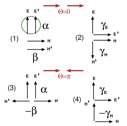
Figure 2: Compton scattering viewed as simultaneous interaction of two electric field vectors ${\bf E,E^{\prime}}$ and magnetic field vectors ${\bf H,H^{\prime}}$ for four different cases. (1) Helicity independent forward Compton scattering as given by the amplitude $f_{0}(\omega)$. (2) Helicity dependent forward Compton scattering as given by the amplitude $g_{0}(\omega)$. (3) Helicity independent backward Compton scattering as given by the amplitude $f_{\pi}(\omega)$. (4) Helicity dependent backward Compton scattering as given by the amplitude $g_{\pi}(\omega)$. Longitudinal photons can only provide two electric vectors with parallel planes of linear polarization as shown in the encircled upper part of panel (1). In panels (2) and (4) the direction of rotation leading from ${\bf E}$ to ${\bf E^{\prime}}$ depends on the helicity difference $|\lambda_{N}-\lambda_{\gamma}|$, being 1/2 or 3/2.

Panel (1) corresponds to the amplitude $f_{0}(\omega)$, panel (2) to the amplitude $g_{0}(\omega)$, panel (3) to the amplitude $f_{\pi}(\omega)$ and panel (4) to the amplitude $g_{\pi}(\omega)$. Panel (1) contains two parallel electric vectors and two parallel magnetic vectors. Through these the electric polarizability $\alpha$ and the magnetic polarizability $\beta$ can be measured. In panel (3) corresponding to backward scattering the direction of the magnetic vector is reversed so that instead of $+\beta$ the quantity $-\beta$ is measured. The nucleon has a spin and because of this the two electric and magnetic vectors have the option of being perpendicular to each other. This leads to the definition of the spin-polarizability $\gamma$ which comes in different versions $\gamma_{E}$ and $\gamma_{H}$, respectively. The different directions of the magnetic field in the forward and backward direction leads to definitions of polarizabilities for the four cases

$$(1)\quad(\alpha+\beta)\hskip 56.9055pt\text{forward polarizability},$$ (32)

$$(2)\quad\gamma_{0}=\gamma_{E}+\gamma_{H}\hskip 25.60747pt\text{forward spin-polarizability},$$ (33)

$$(3)\quad(\alpha-\beta)\hskip 56.9055pt\text{backward polarizability},$$ (34)

$$(4)\quad\gamma_{\pi}=(\gamma_{E}-\gamma_{H})\hskip 17.07164pt\text{backward spin-polarizability}.$$ (35)

3 Resonant and nonresonant spin-dependent and spin-independent cross sections

The $s$-channel degrees of freedom are given by the resonant and nonresonant spin-dependent and spin-independent cross sections for photo-absorption. The most precise information on these cross sections may be obtained from the CGLN amplitudes of meson photoproduction and from the couplings $A_{1/2}$ and $A_{3/2}$ of the nucleon resonant states. The somewhat lengthy procedure to obtain these relations between partial cross sections and the amplitudes is described in detail in the previous paper [7] and should not be repeated here. Instead we give in the following a detailed description of the essential results and refer the reader to the previous work [7] for further details.

3.1 Prediction of nonresonant photo-absorption cross section

In case of the nonresonant contributions we have to take into account the CGLN amplitudes of the multipoles $E_{0+}$, $M^{(3/2)}_{1-}$ and $(M,E)^{(1/2)}_{1+}$. These amplitudes lead to the following partial cross sections

$$\sigma_{1/2}(0+)=\frac{8\pi q}{k}\left[3\left|{}_{(p,n)}E^{(1/2)}_{0+}\right|^{2}+\frac{2}{3}\left|E^{(3/2)}_{0+}\right|^{2}\right],$$ (36)

$$\sigma_{3/2}(0+)=0,$$ (37)

$$\sigma^{(3/2)}_{1/2}(1-)=\frac{8\pi q}{k}\frac{2}{3}\left|M^{(3/2)}_{1-}\right|^{2},$$ (38)

$$\sigma^{(3/2)}_{3/2}(1-)=0,$$ (39)

$$\sigma^{(1/2)}_{1/2}(1+)=\frac{8\pi q}{k}\frac{3}{2}\left|3_{(p,n)}E^{(1/2)}_{1+}+_{(p,n)}M^{(1/2)}_{1+}\right|^{2},$$ (40)

$$\sigma^{(1/2)}_{3/2}(1+)=\frac{8\pi q}{k}\frac{9}{2}\left|{}_{(p,n)}E^{(1/2)}_{1+}-_{(p,n)}M^{(1/2)}_{1+}\right|^{2}$$ (41)

where $q$ and $k$ are the 3-momenta of the pion and the photon in the c.m. system, respectively. From these relations the spin-dependent and spin-independent cross sections can be calculated using available CGLN amplitudes. For the $E_{0+}$ amplitude we obtain the relation

$$\sigma_{3/2}(0+)-\sigma_{1/2}(0+)=-2\,\sigma_{T}(0+).$$ (42)

Eq. (42) shows that the spin-dependent and spin-independent amplitudes corresponding to the $E_{0+}$ multipole are proportional to each other so that the following discussion of $\sigma_{T}(0+)$ implies also the parallel discussion of $\sigma_{3/2}(0+)-\sigma_{1/2}(0+)$.

The contribution of the $E_{0+}$ multipole may be considered as the electric-dipole “pion-cloud” contribution because this is the only electric-dipole amplitude which is given by nonresonant pion photoexcitation. In order to study the driving mechanism for the photoproduction process it is useful to first refer to the Born approximation as represented by the two upper curves in Figure 3. In case of the Born approximation there are two contributions viz. the Kroll-Ruderman term (photoproduction of charged pions on the nucleon) and the pion pole term (photoproduction of a charged pion being emitted by a nucleon). The difference between the cross sections for the proton and the neutron is a consequence of the different dipole moments of the $N\pi$ system in the two cases. For both contributions the pseudovector coupling (PV) constant $f=g_{\pi NN}(m_{\pi}/2m)$ enters into the pion photoproduction matrix element with $g_{\pi NN}=13.169\pm 0.057$ (for more details see [22]).

Figure 3: Spin independent photo-absorption cross section due the $E_{0+}$ amplitude for the neutron (n) and proton (p), respectively. Upper curves: Born approximation. Lower curves: Empirical data.

In Figure 3 the upper cross sections predicted in the Born approximation apparently are much larger than the empirical cross sections. This means that the “pion cloud” contribution to the polarizabilities and spin-polarizabilities cannot simply be understood in terms of the Kroll-Ruderman term and the pion pole term together with the pseudovector coupling constant $f$. Two reasons for the deviation of the empirical $E_{0+}$ amplitude from the Born approximation have been discussed in [23]. The first reason is that the pseudovector (PV) coupling is not valid at high photon energies but has to be replaced by some average of the PV and the pseudoscalar (PS) coupling, or by introducing a formfactor. The second reason are $\rho$- and $\omega$-meson $t$-channel exchanges which are not taken into account in the Born approximation. From these findings we have to conclude that the “pion cloud” contribution to the polarizabilities and spin-polarizabilities cannot be understood in terms of models which only take into account those effects which show up in the low-energy limit.

3.2 Predicted resonant photo-absorption cross sections

For the resonant cross sections in principle also a direct calculation from the CGLN amplitudes is possible provided the one-pion branching $\Gamma_{\pi}/\Gamma_{r}$ of the resonances is taken into account where necessary. However, as shown in [7], a much more precise procedure is available. This procedure makes use of the fact that precise values for total cross-sections $\sigma_{T}$ are easier to obtain than for the cross-section differences $\sigma_{3/2}-\sigma_{1/2}$. Therefore, we start from the relation

$$\sigma^{n}_{3/2}-\sigma^{n}_{1/2}=A_{n}\,\frac{1}{2}\,(\sigma^{n}_{3/2}+\sigma^{n}_{1/2})=A_{n}\,\sigma^{n}_{T}$$ (43)

where $n$ refers to the different resonant states. For the precise prediction of $\sigma^{n}_{T}=\frac{1}{2}\,(\sigma^{n}_{3/2}+\sigma^{n}_{1/2})$ we use the Walker parameterization of resonant states where the cross sections are represented in terms of Lorentzians in the form

$$I=I_{r}\left(\frac{k_{r}}{k}\right)^{2}\frac{W^{2}_{r}\,\Gamma(q)\Gamma^{*}_{\gamma}(k)}{(W^{2}-W^{2}_{r})^{2}+W^{2}_{r}\,\Gamma^{2}(q)}$$ (44)

where $W_{r}$ is the resonance energy of the resonance. The functions $\Gamma(q)$ and $\Gamma^{*}_{\gamma}(k)$ are chosen such that a precise representation of the shapes of the resonances are obtained. The appropriate parameterizations and the related references are given in [7]. Furthermore, some consideration given in [7] shows that the peak cross section can be expressed through the resonance couplings in the following form

$$I_{r}=\frac{2\,m}{W_{r}\Gamma_{r}}\left[|A_{1/2}|^{2}+|A_{3/2}|^{2}\right].$$ (45)

For the total widths $\Gamma_{r}$ and the resonance couplings precise data are available. Tabulations of values adopted for the present purpose are given in [7].

Figure 4: Resonant part of the helicity independent photo-absorption cross-section for the proton and the neutron. Thick line: Sum of all resonances. Thin lines: Contributing single resonances. The energies and strengths corresponding to these resonances are given in Tables 7 and 8 of [7].

Figure 5: Resonant part of the helicity dependent photo-absorption cross-section for the proton and the neutron. Thick line: Sum of all resonances. Thin lines: Contributing single resonances. The energies and strengths corresponding to these resonances are given in Tables 7 and 8 of [7]. The signs of the cross sections are given in Table 3 of [7].

The results obtained for $\sigma_{T}$ and $\sigma_{3/2}-\sigma_{1/2}$ from the present procedure are shown in Figures 4 and 5. The resonance couplings $A_{3/2}$ and $A_{1/2}$, the widths $\Gamma_{r}$ and the scaling factors $A_{n}$ entering into (43) are tabulated in [7]. For the present purpose the scaling factor $A_{n}$ of the $P_{33}(1232)$ resonance, i.e. quantity $A(P_{33}(1232))$ should be discussed in more detail because this resonance provides by far the largest contribution.

For this purpose we start from the relations

$$\sigma^{(3/2)}_{1/2}(1+)=\frac{8\pi q}{k}\frac{1}{3}\left|3E^{(3/2)}_{1+}+M^{(3/2)}_{1+}\right|^{2}(\Gamma_{r}/\Gamma_{\pi})$$ (46)

$$\sigma^{(3/2)}_{3/2}(1+)=\frac{8\pi q}{k}\left|E^{(3/2)}_{1+}-M^{(3/2)}_{1+}\right|^{2}(\Gamma_{r}/\Gamma_{\pi})$$ (47)

where the one-pion branching factor $(\Gamma_{\pi}/\Gamma_{r})$ has been included for completeness only, because this factor is equal to 1 in case of the $P_{33}(1232)$ resonance. The scaling factor $A_{n}$ (see Eq. 43) for the $P_{33}(1232)$ resonance may be obtained in the following way. First we introduce

$$\delta=\left(\frac{E^{(3/2)}_{1+}}{M^{(3/2)}_{1+}}\right)_{\rm res}$$ (48)

and find

$$\sigma^{(3/2)}_{1/2}(1+)=\frac{1}{2}\,\sigma^{(3/2)}_{T}(1+)\,(1+6\,{\rm Re}\,\delta),$$ (49)

$$\sigma^{(3/2)}_{3/2}(1+)=\frac{3}{2}\,\sigma^{(3/2)}_{T}(1+)\,(1-2\,{\rm Re}\,\delta),$$ (50)

$$A(P_{33}(1232))=1-6\,{\rm Re}\,\delta$$ (51)

where use has been made of the reasonable approximation $|\delta|^{2}\ll|{\rm Re}\,\delta|$. We see that $A(P_{33}(1232))=1$ for $\delta=0$, but is strongly dependent on $\delta$ otherwise. The number we get for $\delta$ is strongly dependent on the energy at which we read ${E^{(3/2)}_{1+}}$ and ${M^{(3/2)}_{1+}}$ from available CGLN data. The appropriate choice is to select that energy where the ratio $A(P_{33}(1232))$ obtains its maximum. Using the data in [9] we arrive at

$$A(P_{33}(1232))=1.26\quad\text{and}\quad{\rm Re}\,\delta=-4.4\%.$$ (52)

This value for $A(P_{33}(1232))$ has been tested and found valid when compared with the experimental Mainz data on $\sigma_{3/2}-\sigma_{1/2}$ [7]. Therefore, it is completely justified to use the numbers in Eq. (52) for the calculation of the spin-polarizabilities.

On the other hand the $E2/M1$ ratio given by ${\rm Re}\,\delta$ is larger than the adopted value of REM=$E2/M1$=$-2.2\%$ [9] or REM=$-2.5\%$[10] by approximately a factor of 2. The explanation for this difference is that REM is defined at the resonance energy $W_{r}$ of the nucleon resonance where indeed the smaller value for $E2/M1$ is obtained than the $E2/M1$ ratio corresponding to its maximum. For the comparison of the two different results for the $E2/M1$ ratio it is useful to refer to [24] where it is clearly shown that at the resonance energy $W_{r}=1232$ MeV of the $P_{33}(1232)$ resonance Im $E_{1+}$ is equal to about $50\%$ of this quantity at its maximum which is located at $W=1200$ MeV.

4 Numerical results

Numerical results for the spin-polarizabilities calculated on the basis of the procedure given above and partly also outlined in [7] are given in Table 1.

Table 1: Resonant (lines 2–9), single-pion nonresonant (lines 11–13) and $t$-channel (lines 15–17) components of the spin-polarizabilities in units of $10^{-4}$fm⁴. For the backward spin-polarizabilities $\gamma_{\pi}$ more information may be found in [7].

1		$\gamma^{(p)}_{0}$	$\gamma^{(n)}_{0}$	$\gamma^{(p)}_{\pi}$	$\gamma^{(n)}_{\pi}$	$\gamma^{(p)}_{E}$	$\gamma^{(n)}_{E}$	$\gamma^{(p)}_{M}$	$\gamma^{(n)}_{M}$
2	$P_{33}(1232)$	$-3.03$	$-3.03$	$+5.11$	$+5.11$	$+1.04$	$1.04$	$-4.07$	$-4.07$
3	$P_{11}(1440)$	$+0.05$	$+0.02$	$-0.10$	$-0.04$	$-0.025$	$-0.01$	$+0.075$	$+0.03$
4	$D_{13}(1520)$	$-0.14$	$-0.07$	$-0.39$	$-0.20$	$-0.265$	$-0.135$	$+0.125$	$+0.65$
5	$S_{11}(1535)$	$+0.05$	$+0.01$	$+0.13$	$+0.04$	$+0.09$	$0.025$	$-0.04$	$-0.015$
6	$S_{11}(1650)$	$+0.01$	$+0.00$	$+0.03$	$+0.00$	$+0.02$	$0.00$	$-0.01$	$+0.00$
7	$D_{15}(1675)$	$-0.00$	$-0.00$	$-0.00$	$-0.01$	$+0.00$	$-0.005$	$0.00$	$+0.005$
8	$F_{15}(1680)$	$-0.04$	$-0.00$	$+0.13$	$+0.01$	$+0.045$	$+0.005$	$-0.085$	$-0.005$
9	higher res.	$0.00$	$0.00$	$+0.03$	$+0.03$	$0.015$	$+0.015$	$-0.015$	$-0.015$
10	sum-res.	$-3.09$	$-3.07$	$+4.94$	$+4.94$	$+0.925$	$+0.935$	$-4.015$	$-4.005$
11	$E_{0+}$	$+2.47$	$+3.18$	$+3.75$	$+4.81$	$+3.11$	$+3.995$	$-0.64$	$-0.815$
12	$M^{(3/2)}_{1-}$	$-0.11$	$-0.11$	$-0.18$	$-0.18$	$-0.145$	$-0.145$	$+0.035$	$+0.035$
13	$(M,E)^{(1/2)}_{1+}$	$+0.14$	$+0.38$	$+0.24$	$+0.66$	$+0.19$	$+0.52$	$-0.05$	$-0.14$
14	1$\pi$-nonres.	$+2.51$	$+3.45$	$+3.81$	$+5.29$	$+3.16$	$+4.37$	$-0.65$	$-0.92$
15	$\pi^{0}$-$t$-chan.	$0.00$	$0.00$	$-46.7$	$+46.7$	$-23.35$	$+23.35$	$+23.35$	$-23.35$
16	$\eta$-$t$-chan.	$0.00$	$0.00$	$+1.2$	$+1.2$	$+0.6$	$+0.6$	$-0.6$	$-0.6$
17	$\eta^{\prime}$-$t$-chan.	$0.00$	$0.00$	$+0.4$	$+0.4$	$+0.2$	$+0.2$	$-0.2$	$-0.2$
18	sum $t$-chan.	0.00	0.00	$-45.1$	$+48.3$	$-22.55$	$+24.15$	$+22.55$	$-24.15$
19	$\gamma N\to\pi\Delta$	$0.00$	$0.00$	$-0.28$	$-0.23$	$-0.14$	$-0.115$	$+0.14$	$0.115$
20	tot. sum	$-0.58$	$+0.38$	$-36.6$	$+58.3$	$-18.6$	$+29.3$	$+18.0$	$-29.0$

In this table we order the separate contributions to the spin-polarizabilities in three groups which are the resonant nucleon excitations, the nonresonant nucleon excitations and the $t$-channel contributions. The resonant contributions are dominated by the $P_{33}(1232)$ resonance, the nonresonant nucleon excitations by the $E_{0+}$ amplitude and the $t$-channel by the $\pi^{0}$ pole.

Except for the precision, the advantage of the present method is that it is comparatively easy to arrive at reliable errors. Three errors are relevant, (i) the error of the spin-dependent peak cross section $1.26\times I_{r}$ of the $P_{33}(1232)$ resonance, the error of its width $\Gamma_{r}$ and (ii) the error of the cross section $\sigma(E_{0+}$). These quantities are well investigated, so that a 1$\sigma$ error of $3(4)\%$ for each of these quantities appears to be appropriate without being too optimistic. This leads to $\gamma^{(p)}_{0}=-0.58\pm 0.15(0.20)$ and $\gamma^{(n)}=+0.38\pm 0.17(0.22)$. Taking into account the well-known rules of error analysis these results are not modified by the errors of all the other contributions even in case rather large relative errors of the order of $20-30\%$ are adopted. Therefore, the values

$$\gamma^{(p)}_{0}=-0.58\pm 0.20,\quad\gamma^{(n)}_{0}=+0.38\pm 0.22.$$ (53)

appear to be justified as final results. These final results are also given in the abstract.

For the proton the present result may be compared with the most recent previous evaluation [1]. The main result of this evaluation is $\gamma^{(p)}_{0}=-0.90\pm 0.08\pm 0.11$. Other results based on different photomeson analyses are $\gamma^{(p)}_{0}=-0.67$ (HDT), $-0.65$ (MAID), $-0.86$ (SAID) and $-0.76$ (DMT). In view of the fact that different data sets have been used in these analyses the consistency of these results and the agreement with our result appears remarkably good. A comparison is also possible with the analysis of Drechsel et al. [25] based on CGLN amplitudes and dispersion theory. The numbers obtained are $\gamma^{(p)}_{0}=-0.6$ and $\gamma^{(n)}_{0}=+0.0$ based on the HDT parametrization. The result obtained in [25] for the proton is in close agreement with our result, not only with respect to the total result but also with respect to the partial contributions. The result obtained in [25] for the neutron confirms our result that the quantity $\gamma^{(n)}_{0}$ has the tendency of being shifted towards positive values. In [25] also a detailed comparison with chiral perturbation theory is given which should not be repeated here.

Our present results for the backward spin-polarizabilities may be compared with the predictions of L’vov and Nathan [13] obtained on the basis of the SAID and HDT parameterizations of the CGLN amplitudes. Our result agrees best with the results from the HDT parameterization being $\gamma^{(p)}_{\pi}=-37.0$ and $\gamma^{(n)}=+57.8$. From these comparisons we conclude that the predicted spin-polarizabilities are satisfactorily known as far as their numerical values are concerned.

After obtaining this high precision for the predicted backward spin-polarizabilities a reconsideration of the corresponding experimental data is advisable. For the neutron the result $\gamma^{(n)}_{\pi}=58.6\pm 4.0$ given before [2] still remains its validity because there are no further data available. For the proton three experiments of high precision [26, 27],[28] and [29] have been carried out to determine $\gamma^{(p)}_{\pi}$. As mentioned above the evaluation of the data requires the use of CGLN parameterizations to represent the Compton amplitudes, in addition to the spin-polarizability $\gamma_{\pi}$ which is treated as an adjustable parameter. This procedure implies that the determination of $\gamma_{\pi}$ becomes to some extent model dependent. In our previous determination of a recommended final result [2] all the available data have been included in the weighted average though some of them showed large deviations from the majority of the data, which can be traced back to inconsistencies in the respective CGLN parameterizations. Details may be found in section 5.2 of Ref. [2]. Figure 14 contained in the same section of Ref. [2] explains why results of an early experiment [30] cannot be included in the averaging procedure. Omitting now evaluations with obvious inconsistencies the selection of data shown in Table 2 is obtained.

Table 2: Reevaluation of the experimental backward spin-polarizability of the proton: The present average over experimental data differs from the previous one [2] because some evaluations of the data measured in [26, 27] and [29] have been excluded because of systematic inconsistencies in the CGLN amplitudes.

$\gamma^{(p)}_{\pi}$	reference
$-37.1\pm 3.0$	[26, 27]
$-35.9\pm 2.3$	[28]
$-36.5\pm 2.5$	[29]
$-36.4\pm 1.5$	weighted average

We propose to use the weighted average shown in Table 2 as the updated recommended value for the backward spin-polarizability of the proton.

5 Some properties of the polarizabilities and spin-polarizabilities

The final goal of the ongoing research is to eventually understand the polarizabilities and spin-polarizabilities in terms of models of the nucleon. We do not present a final solution for this problem in the present paper. However, as a first step we investigate some properties of the polarizabilities and spin-polarizabilities which may be helpful for reaching the final goal. A reasonable tool appears to us to compare some properties of polarizabilities and spin-polarizabilities with each other.

5.1 Spin-polarizabilities compared with the electric and magnetic polarizabilities

The introduction of electric ($\gamma_{E}$) and magnetic ($\gamma_{M}$) spin-polarizabilities makes it possible to compare these quantities with the electric ($\alpha$) and magnetic ($\beta$) polarizabilities. This is carried out in Tables 3 and 4. In Table 3 we investigate how the for quantities $\alpha(E_{0+})$, $\beta(E_{0+})$, $\gamma_{E}(E_{0+})$

Table 3: Electric and magnetic polarizabilities and spin-polarizabilities corresponding to the excitation of the nonresonant $E_{0+}$ multipole.

dispersion integral	proton	neutron	unit
$\alpha(E_{0+})=\frac{1}{4\pi^{2}}\int\left[1+\sqrt{1+\frac{2\omega}{m}}\right]\sigma^{(E_{0+})}_{T}(\omega)\frac{d\omega}{\omega^{2}}$	+3.19	+4.07	$10^{-4}$ fm3
$\beta(E_{0+})=\frac{1}{4\pi^{2}}\int\left[1-\sqrt{1+\frac{2\omega}{m}}\right]\sigma^{(E_{0+})}_{T}(\omega)\frac{d\omega}{\omega^{2}}$	–0.34	–0.43	$10^{-4}$ fm3
$\gamma_{E}(E_{0+})=\frac{1}{4\pi^{2}}\int\left[1+\sqrt{1+\frac{2\omega}{m}}(1+\frac{\omega}{m})\right]\sigma^{(E_{0+})}_{T}(\omega)\frac{d\omega}{\omega^{3}}$	+3.11	+4.00	$10^{-4}$ fm4
$\gamma_{M}(E_{0+})=\frac{1}{4\pi^{2}}\int\left[1-\sqrt{1+\frac{2\omega}{m}}(1+\frac{\omega}{m})\right]\sigma^{(E_{0+})}_{T}(\omega)\frac{d\omega}{\omega^{3}}$	–0.64	–0.82	$10^{-4}$ fm4

Table 4: Electric and magnetic polarizabilities and spin-polarizabilities corresponding to resonant excitation of the $P_{33}(1232)$ resonance.

dispersion integral	proton	neutron	unit
$\alpha(P_{33})=\frac{1}{4\pi^{2}}\int\left[1-\sqrt{1+\frac{2\omega}{m}}\right]\sigma^{(P_{33})}_{T}(\omega)\frac{d\omega}{\omega^{2}}$	$-1.07$	$-1.07$	$10^{-4}$ fm3
$\beta(P_{33})=\frac{1}{4\pi^{2}}\int\left[1+\sqrt{1+\frac{2\omega}{m}}\right]\sigma^{(P_{33})}_{T}(\omega)\frac{d\omega}{\omega^{2}}$	$+8.32$	$+8.32$	$10^{-4}$ fm3
$\gamma_{E}(P_{33})=-\frac{A(P_{33})}{8\pi^{2}}\int\left[1-\sqrt{1+\frac{2\omega}{m}}(1+\frac{\omega}{m})\right]\sigma^{(P_{33})}_{T}(\omega)\frac{d\omega}{\omega^{3}}$	$+1.04$	$+1.04$	$10^{-4}$ fm4
$\gamma_{M}(P_{33})=-\frac{A(P_{33})}{8\pi^{2}}\int\left[1+\sqrt{1+\frac{2\omega}{m}}(1+\frac{\omega}{m})\right]\sigma^{(P_{33})}_{T}(\omega)\frac{d\omega}{\omega^{3}}$	$-4.07$	$-4.07$	$10^{-4}$ fm4

and $\gamma_{M}(E_{0+})$ are related to the cross section $\sigma^{(E_{0+})}_{T}$. First of all we notice that dispersion integrals of very similar structure are obtained for the polarizabilities and spin-polarizabilities. In the limit $m\to\infty$ only the electric parts $\alpha$ and $\gamma_{E}$ are different from zero. This means that the nonzero values obtained for $\beta$ and $\gamma_{M}$ may be understood in terms of “relativistic” or “recoil” effects. In a classical model the quantity $\alpha$ corresponds to an electric dipole moment induced in the “pion cloud” through the action of a first electric field vector E. This dipole moment interacts with an electric field vector E’ being parallel to the direction of the first electric field vector E. The main difference between the electric polarizability $\alpha$ and the electric spin-polarizability $\gamma_{E}$ is that for the latter quantity the second electric field vector E’ is perpendicular to the first one. It certainly is a challenge for further research to find a model which explains the relative sizes of the quantities $\alpha(E_{0+})$ and $\gamma_{E}(E_{0+})$. A model like this may be expected to contain valuable information on the dynamics of the excitation of the “pion cloud”.

In Table 4 it is investigated how the quantities $\alpha(P_{33})$, $\beta(P_{33})$, $\gamma_{E}(P_{33})$ and $\gamma_{M}(P_{33})$ are related to the cross section $\sigma^{(P_{33})}_{T}$ corresponding to the $P_{33}(1232)$ resonance. In this case the quantities $\beta(P_{33})$ and $\gamma_{M}(P_{33})$ are the large quantities whereas the quantities $\alpha(P_{33})$ and $\gamma_{E}(P_{33})$ are small “relativistic” or “recoil” corrections. The most interesting difference between the polarizabilities and the spin-polarizabilities is the enhancement factor $A(P_{33}(1232))$ which enters into the spin-polarizabilities but does not enter into the polarizabilities. This enhancement factor has been discussed in detail in subsection 3.2. Since this factor differs from $A(P_{33}(1232))$=1 only because of the nonzero $\delta=E^{(3/2)}_{1+}/M^{(3/2)}_{1+}$ ratio, it is of interest to study the quantity $\delta$ in terms of a model in order to eventually obtain a deeper insight into the driving mechanisms connected with the spin-polarizabilities. This is carried out in the next subsection.

5.2 Experimental and predicted resonance couplings $A_{3/2}$ and $A_{1/2}$ for the $P_{33}(1232)$ resonance

The resonance couplings are quantities which on the one hand can be determined from experimental CGLN amplitudes and on the other hand can be predicted in models of the nucleon. Of these the SU(6)$\times$O(3) harmonic oscillator model has been investigated in detail. Therefore, the resonance couplings predicted in the framework of this model are suitable for relating the resonant components of the spin-polarizabilities to a model of the nucleon.

On the side of the experimental data the resonance couplings are given by

$$A_{1/2}(1+)=-\frac{1}{2}\left[3{\bar{E}}^{(3/2)}_{1+}+{\bar{M}}^{(3/2)}_{1+}\right],$$ (54)

$$A_{3/2}(1+)=\frac{1}{2}\sqrt{3}\left[{\bar{E}}^{(3/2)}_{1+}-{\bar{M}}^{(3/2)}_{1+}\right]$$ (55)

where

$$({\bar{E}}^{(3/2)}_{1+},{\bar{M}}^{(3/2)}_{1+})=\sqrt{\frac{2}{3}}\left[\frac{4\pi\,q_{r}\,W_{r}\,\Gamma^{2}_{r}}{k_{r}\,m\,\Gamma_{\pi}}\right](E^{(3/2)}_{1+},M^{(3/2)}_{1+})$$ (56)

and where $q_{r}$ and $k_{r}$ are the 3-momenta $q$ and $k$ at the resonance maximum. This leads to

$${\rm REM}=\frac{A_{1/2}(1+)-\frac{1}{\sqrt{3}}A_{3/2}(1+)}{A_{1/2}(1+)+\sqrt{3}A_{3/2}(1+)}=\frac{E^{(3/2)}_{1+}}{M^{(3/2)}_{1+}}.$$ (57)

Experimental data given in the literature may be found in Table 5.

Table 5: Experimental resonance couplings $A_{1/2}$ and $A_{3/2}$ in units of $10^{-3}$GeV^-1/2 for the $P_{33}(1232)$ resonance taken from recent publications. The result given by [31] has been adopted in [7] and in the present work to calculate the $\sigma_{T}(P_{33}(1232))$.

$A_{1/2}$	$A_{3/2}$	$E2/M1$ $(\%)$	Ref.	$E2/M1$ $(\%)$ Eq.(57)
$-135\pm 6$	$-250\pm 8$	$-2.5\pm 0.5$	[10]	$-1.6$
$-139.1\pm 3.6$	$-257\pm 4.6$	$-$	[31]	$-1.6$
$-140$	$-265$	$-2.2$	[9]	$-2.2$

The $E2/M1$ ratios given in column 3 of Table 5 are the ones given by the authors listed in column 4, whereas the $E2/M1$ ratios given in column 5 are calculated using Eq. (57). By comparing the results given in columns 3 and 5 we see that there is only partly consistency between these two types of data. This shows that our present procedure to calculated $\sigma_{T}$ from the resonance couplings but not $\sigma_{3/2}$ and $\sigma_{1/2}$ separately is justified. In [7] we have adopted the results given by [31] because of their precision and because these results exactly reproduce the value $I_{r}(P_{33}(1232))=390$ $\mu$b directly determined in a photo-absorption experiment [32].

On the side of the theory the relevant helicity amplitudes for $N\to N^{*}$ transitions induced by the absorption of a real photon are (see e.g. [33])

$$A_{1/2}=\langle N^{*}_{j,+\frac{1}{2}}|H_{\rm int}|N_{\frac{1}{2},-\frac{1}{2}}\rangle$$ (58)

$$A_{3/2}=\langle N^{*}_{j,+\frac{3}{2}}|H_{\rm int}|N_{\frac{1}{2},+\frac{1}{2}}\rangle$$ (59)

where $H_{\rm int}$ is the single-particle interaction Hamiltonian. In a SU(6)$\times$O(3) quark model the resonance couplings for the $N(939)\to P_{33}(1232)$ are given by [34]

$$A_{1/2}=-\frac{2\sqrt{2}}{3}\mu\,\sqrt{\pi\,k}\,R^{s}_{00},$$ (60)

$$A_{3/2}=-2\sqrt{\frac{2}{3}}\mu\,\sqrt{\pi\,k}\,R^{s}_{00}$$ (61)

with

$$R^{s}_{00}=\exp{(-k^{2}/6\alpha^{2})}$$ (62)

where $\mu=0.13$ GeV^-1 is the quark scale magnetic moment in Gaussian units, chosen to fit the magnetic moment of the proton and $\alpha^{2}=0.17$ GeV². The $g$ factor of the quarks is chosen to be $g=1$. Predicted results are given in Table 6.

Table 6: Predicted resonance couplings $A_{1/2}$ and $A_{3/2}$ in units of $10^{-3}$GeV^-1/2 for the $P_{33}(1232)$ resonance taken from previous work.

1	$A_{1/2}$	$A_{3/2}$	Ref.
2	$-101$	$-175$	Copley et al. [34] (nonrel.)
3	$-108$	$-187$	Feynman et al. [35] (rel.)
4	$-103$	$-178$	Feynman et al. [35] (nonrel.)
5	$-113$	$-195$	Close, Li [36] (rel.)
6	$-101$	$-173$	Close, Li [36] (nonrel.)
7	$-108$	$-186$	Capstick [37] (rel.)
8	$-109.7$	$-189.3$	average relativistic prediction
9	$-139$	$-257$	exp. adopted [7]

The results given in lines 2, 4 and 6 correspond to the formulae (60) – (62) and are named nonrelativistic results in the literature. The results in lines 3, 5 and 7 contain relativistic corrections of different kinds. In the paper of Feynman et al. [35] the nonrelativistic harmonic oscillator Hamiltonian is replaced by a relativistic or relativized version by introducing the 4-momenta of the quarks instead of 3-momenta and by introducing coordinate operators. The results obtained in this way for the resonance couplings are about $5\%$ larger than the nonrelativistic results but still about $30-40\%$ smaller than the experimental values. Similar findings have been made by Close and Li [36] and by Capstick [37]. In the paper of Close and Li [36] relativistic corrections due to spin-orbit coupling are taken into account. In the paper of Capstick [37] an electromagnetic transition operator containing relativistic corrections is introduced in addition to relativized quark-model wave functions. We see that the experimental data (line 9) are much larger than the predicted data independent of the specific method of calculation. This means that relativistic corrections cannot explain the large gap between the experimental and theoretical results so that something else must be the reason.

Calculating the photon decay widths from the resonance couplings given in lines 8 and 9 of Table 6 we arrive at

$$\frac{\Gamma_{\gamma}({\rm theor.)}}{\Gamma_{\gamma}({\rm exp.)}}\simeq 0.56.$$ (63)

This means that the single particle model leads to a much too small photon decay width independent of the inclusion or omission of relativistic corrections into the calculation. This discrepancy comes not as a surprise because the quarks in the nucleon are strongly coupled to each other so that the single particle transition should be accompanied by a collective component. This finding is a well-known phenomenon in nuclear physics. Furthermore, this picture also allows to qualitatively explain the electric quadrupole ($E2$) component of the transition which in a single particle model is difficult to understand. In connection with the $E2$ component our present study of the spin-polarizabilities has added an interesting further insight. The $E2/M1$ ratio relevant for the enhancement of the cross-section difference $\sigma_{3/2}-\sigma_{1/2}$ is ${\rm Re}\,\delta=-0.044$ and thus a factor of 2 larger that the standard value REM$=-0.022$. The reason for this difference is that $\delta$ is defined to be the maximum possible $E2/M1$ ratio obtained from the experimental CGLN amplitude whereas the REM$=-0.022$ is determined at the energy $W_{r}$, i.e. the resonance energy of the Lorentzian describing the nucleon resonance.

The results obtained in the foregoing may be summarized by making use of Eqs. (49) and (50). This leads to

$$\sigma_{1/2}^{(3/2)}(1+)=\frac{1}{2}\,\sigma^{(3/2)}_{T}(1+)\,\Big{(}0.56(M1_{\rm sp})+0.44(M1_{\rm coll})\Big{)}\Big{(}1-0.26(E2_{\rm coll})\Big{)},$$ (64)

$$\sigma_{3/2}^{(3/2)}(1+)=\frac{3}{2}\,\sigma^{(3/2)}_{T}(1+)\,\Big{(}0.56(M1_{\rm sp})+0.44(M1_{\rm coll})\Big{)}\Big{(}1+0.09(E2_{\rm coll})\Big{)},$$ (65)

$$\sigma_{3/2}^{(3/2)}(1+)-\sigma_{1/2}^{(3/2)}(1+)=1.26\,\sigma^{(3/2)}_{T}(1+).$$ (66)

The cross sections $\sigma_{1/2}^{(3/2)}(1+)$ and $\sigma_{3/2}^{(3/2)}(1+)$ entering into $\sigma_{3/2}^{(3/2)}(1+)-\sigma_{1/2}^{(3/2)}(1+)$ and, therefore, also into the $P_{33}(1232)$ component of the spin-polarizabilities are composed of single-particle (sp) parts and collective (coll) parts. The single-particle parts have tentatively been identified with the prediction of the SU(6)$\times$O(3) harmonic oscillator model. The difference between this prediction and the experimental total cross section $\sigma^{(3/2)}_{T}(1+)$ is tentatively interpreted as being due to a collective excitation mode which may be understood as being due to a consequence of the strong coupling between the constituent quarks. This spin-dependent strong coupling also leads to a $E2$-component of the electromagnetic transition which diminishes the cross section $\sigma_{1/2}^{(3/2)}(1+)$ by $26\%$ and increases the cross section $\sigma_{3/2}^{(3/2)}(1+)$ by $9\%$. In total we arrive at the cross-section difference given in Eq. (66). The foregoing discussion may be compared with the work of Jenkins and Manohar [38] where relations among the baryon magnetic and transition magnetic moments are derived in the $1/N_{c}$ expansion. These results might be interpreted as suggesting that the single-particle picture works quite well – at least in the case of isovector $M1$ excitations of octet and decouplet baryons. More insights into the dynamics of the $P_{33}(1232)$ resonance and of the $E_{0+}$ amplitude may be found in [19, 20, 21, 39].

6 Summary and discussion

In the foregoing paper we have predicted spin-polarizabilities for the proton and the neutron and compared them with experimental data. Furthermore, we have related the spin-polarizabilities to excitation processes which for the $s$-channel is dominated by the nonresonant $E_{0+}$ amplitude and the $P_{33}(1232)$ nucleon resonance. The $t$-channel contributions is dominated by the $\pi^{0}$ pole contribution. It has been found to be very useful to introduce the spin-polarizabilities $\gamma_{E}$ and $\gamma_{M}$, where the first quantity can be attributed to a two-photon process with two perpendicular electric-field vectors and the second to a two-photon process with two perpendicular magnetic-field vectors. It is shown that the nonresonant $E_{0+}$ amplitude makes a sizable contribution to $\gamma_{E}$, accompanied by a small relativistic correction to $\gamma_{M}$. For the resonant contribution provided by the $P_{33}(1232)$ resonance the multipolarity dependence is opposite as expected. A deeper insight into the dynamics of the $E_{0+}$ and $P_{33}(1232)$ nucleon resonance contributions of the spin-polarizabilities appear possible within models of the nucleon. In case of the $E_{0+}$ amplitude a model has to be found which relates the electric-dipole moment induced in the direction of the first electric vector ${\bf E}$ to a related electric dipole-moment in the direction of the second electric vector ${\bf E}^{\prime}$ being perpendicular to ${\bf E}$. In case of the $P_{33}(1232)$ resonance an appropriate basis for a discussion is provided by the SU(6)$\times$O(3) harmonic oscillator model. It is shown that this model predicts cross sections $\sigma_{1/2}^{(3/2)}(1+)$ and $\sigma_{3/2}^{(3/2)}(1+)$ which amount to only $56\%$ of the $M1$ component of the corresponding experimental cross sections. This observation leads in a natural way to the supposition that the strong coupling between the constituent quarks leads to a collective $M1$ component, filling the gap of $44\%$ between single-particle prediction and the $M1$ part of the experimental cross section. In addition to the effects on the $M1$ excitation, the spin-dependence of the strong coupling between the constituent quarks leads to an $E2$ component, and through this to a diminishing of the $\sigma_{1/2}^{(3/2)}(1+)$ cross section by $26\%$ and to an increase of the $\sigma_{3/2}^{(3/2)}(1+)$ cross-section by $9\%$. These effects together lead to an increase of the cross-section difference $\sigma_{3/2}^{(3/2)}(1+)-\sigma_{1/2}^{(3/2)}(1+)$ by $26\%$ in agreement with spin-dependent cross section measurements carried out at MAMI (Mainz) [40, 7]. For the magnetic spin-polarizability $\gamma_{M}$ this means that the $E2$ excitation also leads to an increase by $26\%$.

References

- [1] B. Pasquini, P. Pedroni, D. Drechsel, Phys. Lett. B 687 (2010) 160, arXiv:1001.4230 [hep-ph].
- [2] M. Schumacher, Progr. Part. Nucl. Phys. 55 (2005) 567, arXiv:hep-ph/0501167.
- [3] M. Schumacher, Eur. Phys. J. A 30 (2006) 413, Eur. Phys. J. A 32 (2007) 121 (E), arXiv:hep-ph/0609040; M.I. Levchuk, A.I. L’vov, A.I. Milstein, M. Schumacher, Proceedings of the Workshop on the Physics of Excited Nucleons, NSTAR 2005 (2005) 389, arXiv:hep-ph/0511193.
- [4] M. Schumacher, Eur. Phys. J. A 31 (2007) 327, arXiv:0704.0200 [hep-ph].
- [5] M. Schumacher, Eur. Phys. J. A 34 (2007) 293, arXiv:0712.1417 [hep-ph].
- [6] M. Schumacher, AIP Conference Proceedings 1030 (Workshop on Scalar Mesons and Related Topics Honoring Michael Scadrons’s 70th Birthday - SCADRON70) (2008) 129, arXiv:0803.1074 [hep-ph] and arXiv:0805.2823 [hep-ph].
- [7] M. Schumacher, Nucl. Phys. A 826 (2009) 131, arXiv:0905.4363 [hep-ph].
- [8] M. Schumacher, Eur. Phys. J. C 67 (2010) 283, arXiv:1001.0500 [hep-ph].
- [9] D. Drechsel, S.S. Kamalov, L. Tiator, Eur. Phys. J. A 34 (2007) 69, arXiv:0710.0306 [nucl-th].
- [10] K. Nakamura et al. (Particle Data Group), J. Phys. G 37 (2010) 075021.
- [11] A.I. L’vov, V.A. Petrun’kin, M. Schumacher, Phys. Rev. C 55 (1997) 359.
- [12] D. Drechsel, B. Pasquini, M. Vanderhaeghen, Phys. Rep. 378 (2003) 99.
- [13] A.I. L’vov, A.M. Nathan, Phys. Rev. C 59 (1999) 1064.
- [14] A.C. Hearn, E. Leader, Phys. Rev. 126 (1962) 789; R. Köberle, Phys. Rev. 166 (1968) 1558.
- [15] I. Caprini, G. Colangelo, H. Leutwyler, Phys. Rev. Lett. 96 (2006) 132001, arXiv:hep-ph/0512364.
- [16] N.A. Törnqvist, Z. Phys. C 68 (1995) 647.
- [17] M. Boglione, M.R. Pennington, Phys. Rev. D 65 (2002) 114012, arXiv:hep-ph/0203149.
- [18] D. Babusci, G. Giordano, A.I. L’vov, G. Matone, A.M. Nathan, Phys. Rev. C 58 (1998) 1013.
- [19] B.R. Holstein, D. Drechsel, B. Pasquini, M. Vanderhaeghen, Phys. Rev. C 61 (2000) 034316, arXiv:hep-ph/9910427.
- [20] R.P. Hildebrandt, H.W. Grießhammer, T.R. Hemmert, B. Pasquini, Eur. Phys. J. A 20 (2004) 293, arXiv:nucl-th/0307070.
- [21] R.P. Hildebrandt, H.W. Grießhammer, T.R. Hemmert, Eur. Phys. J. A 20 (2004) 329, arXiv:nucl-th/0308054.
- [22] T. Ericson, W. Weise, Pions and Nuclei, Int. Ser. Monogr. Phys., Vol. 74 (Oxford Science Publications, 1988).
- [23] D. Drechsel, S.S. Kamalov, G. Krein, L. Tiator, Phys. Rev. D 59 (1999) 094021.
- [24] L. Tiator, D. Drechsel, O. Hanstein, S.S. Kamalov, S.N. Yang, Nucl. Phys. A 689 (2001) 205, arXiv:nucl-th/0012046.
- [25] D. Drechsel, G. Krein, O. Hanstein, Phys. Lett. B 420 (1998) 248, arXiv:nucl-th/9710029.
- [26] G. Galler et al., Phys. Lett. B 501 (2001) 245.
- [27] S. Wolf et al., Eur. Phys. J. A 12 (2001) 231.
- [28] V. Olmos de León et al., Eur. Phys. J. A 10 (2001) 207.
- [29] M. Camen et al., Phys. Rev. C 65 (2002) 032202.
- [30] J. Tonnison et al., Phys. Rev. Lett. 80 (1980) 4382; G. Blanpied et al., Phys. Rev. C 64 (2001) 025203.
- [31] M. Dugger, et al., Phys. Rev. C 76 (2007) 025211.
- [32] T.A. Armstrong, et al., Nucl. Phys. B41 (1972) 445.
- [33] A.W. Thomas, W. Weise, The Structure of the Nucleon Wiley-VCH, Berlin 2000.
- [34] L.A. Copley, G. Karl, E. Obryk, Phys. Lett. 29B (1969) 117; Nucl. Phys. B13 (1969) 303.
- [35] R.P. Feynman, M. Kislinger, F. Ravndal, Phys. Rev. D 3 (1971) 2706.
- [36] F.E. Close, Z. Li, Phys. Rev. D 42 (1990) 2194.
- [37] S. Capstick, Phys. Rev. D 46 (1992) 2864.
- [38] E. Jenkins, A.N. Manohar, Phys. Lett. B 335 (1994) 452.
- [39] V. Pascalutsa, M. Vanderhaeghen, S.-N. Yang, Phys. Rept. 437 (2007) 125, arXiv:hep-ph/0609004.
- [40] GDH Collaboration, J. Ahrens, et al., Phys. Rev. Lett. 87 (2001) 022003, arXiv:hep-ex/0105089.