Hyperfine, rotational and Zeeman structure of the lowest vibrational levels of the ⁸⁷Rb₂ $(1)\,^{3}\Sigma_{g}^{+}$ state

Abstract

We present the results of an experimental and theoretical study of the electronically excited $(1)\,^{3}\Sigma_{g}^{+}$ state of ⁸⁷Rb₂ molecules. The vibrational energies are measured for deeply bound states from the bottom up to $v^{\prime}=15$ using laser spectroscopy of ultracold Rb₂ Feshbach molecules. The spectrum of each vibrational state is dominated by a 47 GHz splitting into a $0_{\textrm{g}}^{-}$ and $1_{\textrm{g}}$ component caused mainly by a strong second order spin-orbit interaction. Our spectroscopy fully resolves the rotational, hyperfine, and Zeeman structure of the spectrum. We are able to describe to first order this structure using a simplified effective Hamiltonian.

I Introduction

Progress in the field of ultracold atomic and molecular gases has always been strongly linked to developments in molecular spectroscopy. Photoassociation spectroscopy, for example, has been important for studies of ultracold atomic collisions and for production of ultracold molecules Wei99 ; Jon06 ; Koh06 ; Sage2005 . In 2008, after carrying out spectroscopic searches, several groups managed to produce cold and dense samples of deeply bound molecules in well-defined quantum states La08 ; Ni08 ; Dan08 ; Vit08 ; Dei08 ; Ospelkaus2010 . For this, a variety of clever optical transfer and filtering schemes were developed which involved electronically excited molecular levels. These levels had to be properly chosen for high efficiency and selectivity of molecule production. This will also be the case for future experiments involving cold collisions Ospelkaus2010b ; Ni2010 , ultracold chemistry Sta06 ; Kre05 ; Kre08 , and testing fundamental laws via precision spectroscopy Ze08 ; DeM08 ; Ch09 . A detailed understanding of the excited molecular potentials is therefore necessary. Very recent work Bai11 investigated the spin-orbit-coupled $A^{1}\Sigma_{u}^{+}$ and $b^{3}\Pi_{u}$ states of Cs₂. In other work a detailed analysis of weakly bound Rb₂ levels of the excited $1_{g}$ state close to the $5S_{1/2}+5P_{1/2}$ dissociation limit is currently under way Ber11 (see also related work in Fig. 13 of Jon06 ).

Here we present measurements and analysis for deeply bound ($v^{\prime}=0...15$) levels of the $(1)\,^{3}\Sigma_{g}^{+}$ (5$P_{1/2}$ + 5$S_{1/2})$ state of ⁸⁷Rb₂. This state is relevant for the production of deeply bound molecules in the $a^{3}\Sigma_{u}^{+}$ state via stimulated Raman adiabatic passage La08 ; Win07 . The $a^{3}\Sigma_{u}^{+}$ state is the energetically lowest triplet potential, giving rise to long lived molecules which are of interest for cold collision experiments. The levels of the $a^{3}\Sigma_{u}^{+}$ state have been mapped out and identified in detail in a recent publication Str10 .

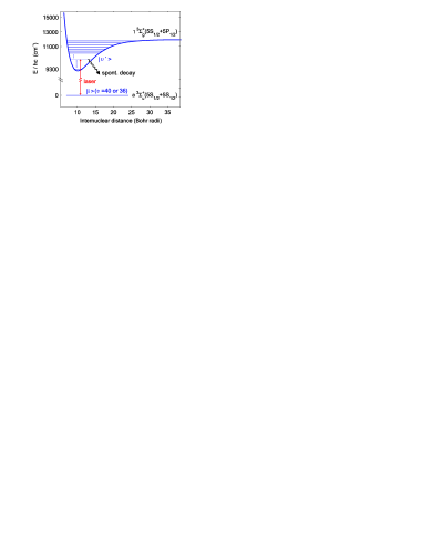
Figure 1: Spectroscopy scheme. A tunable laser couples the Feshbach molecule level $|i\rangle$ to an excited level $|v^{\prime}\rangle$ with energy $E$ in the $(1)\,^{3}\Sigma_{g}^{+}$ state. The excited state quickly decays spontaneously. Level positions in the $(1)\,^{3}\Sigma_{g}^{+}$ potential are detected through resonantly enhanced loss of Feshbach molecules. $h$ is Planck’s constant and c is the speed of light.

The $(1)\,^{3}\Sigma_{g}^{+}$ state is not easily accessible in conventional setups since the molecules in a Rb₂ gas at ambient temperatures are found in the $X^{1}\Sigma_{g}^{+}$ ground state. Electric dipole transitions from this state to the $(1)\,^{3}\Sigma_{g}^{+}$ state are forbidden by the $g\leftrightarrow{}u$ symmetry selection rule. As a consequence it has only quite recently become possible to explore in detail the Rb₂ $(1)\,^{3}\Sigma_{g}^{+}$ state. Lozeille et al. L06 performed photoionization spectroscopy of ultracold Rb₂ molecules produced by photoassociation in a magneto-optical trap to resolve the large $0_{\textrm{g}}^{-}-1_{\textrm{g}}$ splitting of the vibrational levels. Mudrich et al. Mu10 used pump-probe photoionization spectroscopy of Rb₂ formed on helium nanodroplets to measure the vibrational progression of deeply bound levels. Our work goes beyond this as we fully resolve the rotational, hyperfine, and Zeeman structure of the Rb₂ levels in the $(1)\,^{3}\Sigma_{g}^{+}$ state.

The starting point for our experiments is an ultracold ensemble of weakly bound Rb₂ Feshbach molecules in a well defined quantum level, which has contributions from both the $(1)\,^{3}\Sigma_{g}^{+}$ and $X^{1}\Sigma_{g}^{+}$ states. A scanning laser with sub-MHz short-term linewidth drives a one-photon transition to levels in the $(1)\,^{3}\Sigma_{g}^{+}$ state (see Fig. 1). We obtain loss spectra for various magnetic fields from 0 to 1000 G. The data are well described by an effective Hamiltonian which contains terms for molecular rotation as well as spin-spin, hyperfine, and Zeeman interactions.

The article is organized as follows. Section II of our article presents the experimental setup for the Rb₂ spectroscopy. In section 3 we show typical measured spectra and discuss their main features. Section IV presents the model that we use to describe our data. Section V explains the detailed level structure of our data based on the model. We conclude with a summary and a short outlook in section VI.

II Experimental setup

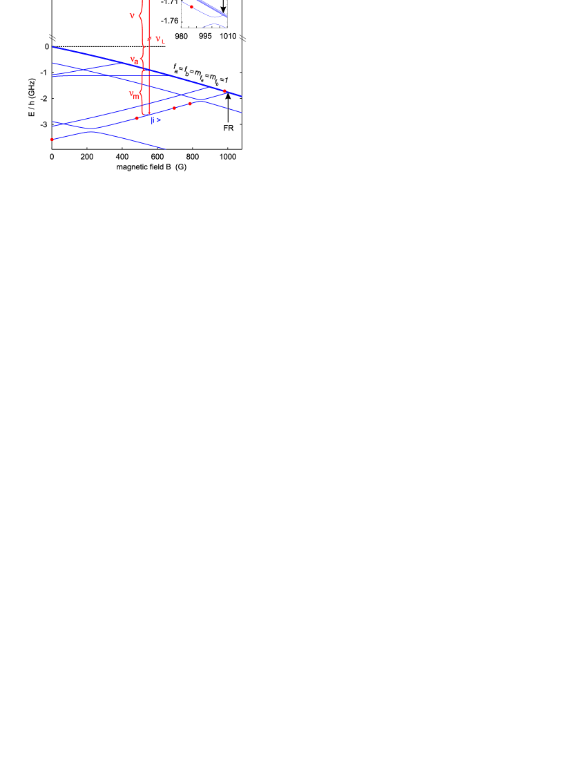
Figure 2: Energy diagram of the Zeeman structure for some weakly bound Rb₂ molecular states below the $|f_{a}=1,m_{f_{a}}=1\rangle$ + $|f_{a}=b,m_{f_{b}}=1\rangle$ atomic asymptote. Dots mark the levels and magnetic fields used for the spectroscopy. For simplicity, throughout the paper we report excitation frequencies $\nu$ with respect to the two-atom threshold at 0 G. These are obtained by subtracting the known atomic Zeeman shift $\nu_{a}$ and the known molecular binding frequency $\nu_{m}$ from the excitation frequency $\nu_{L}$. The inset zooms into the region near the Feshbach resonance at 1007.4 G, marked with an arrow and ”FR”.

Feshbach molecules in state $|i\rangle$ are irradiated by a pulse of light from a continuous-wave laser the wavelength of which is slowly scanned over the range 1000 to 1050 nm (Fig. 1). The laser beam has an $1/e^{2}$ intensity waist radius of 130 $\mu$m at the molecular sample. It is linearly polarized along the magnetic bias field $\mathbf{B}$ (parallel to gravity) and thus can only induce $\pi$ transitions. The light pulse typically lasts for 50 ms and has a rectangular temporal shape. When resonant with an $|i\rangle-|v^{\prime}\rangle$ transition, our laser induces losses in the Feshbach population due to excitation to $|v^{\prime}\rangle$ and subsequent fast (ns) decay to unobserved states. For each data point, a new ensemble of Feshbach molecules has to be prepared, a process which typically requires 28 s.

The preparation of the Feshbach molecules is described in detail in Tha06 ; La08a . In brief, following laser cooling and evaporative cooling, we trap an ultracold atomic cloud of 3$\times 10^{5}$ ⁸⁷Rb atoms close to quantum degeneracy in a 3D optical lattice. A sizeable fraction ($\approx 1/3$) of the lattice sites are doubly occupied and the atoms are trapped in the lowest Bloch band. Afterwards, we ramp over a Feshbach resonance at a magnetic field of 1007.4 G (1 G = 10^-4 T) (see Fig. 2) Vol03 to obtain $3\times 10^{4}$ Feshbach molecules with no more than a single molecule per lattice site. The lattice depth for the Feshbach molecules is deep enough to prevent the molecules from colliding with each other, and we observe lifetimes of up to a few hundred ms.

In order to investigate the Zeeman structure of the levels in the $1^{3}\Sigma_{g}^{+}$ state, we carry out the spectroscopy at various magnetic fields between 0 and 1000 G. Thus, after we have produced the Feshbach molecules, the magnetic field is ramped down from 1007.4 G to its chosen value. When doing so, one has to keep track of the quantum state $|i\rangle$ of the Feshbach molecules as well as their binding energy as they both change in general with magnetic field. Fig. 2 shows a number of relevant weakly bound molecular energy levels which exhibit many avoided crossings. When ramping over such a crossing, the molecules could potentially end up in two different quantum levels. This would be problematic for the spectroscopy and is avoided as described below.

A large fraction of our measurements are carried out at 986.8 G with a binding energy of 22.7 MHz$\times h$ (see inset of Fig. 2). The corresponding Feshbach state is best described in the atomic basis and correlates to $|v=40,(f_{a}=1,f_{b}=1)f=2,l=0,F=2,M=2\rangle$ at low magnetic fields. Here $v$ is the vibrational quantum number of the $a^{3}\Sigma_{u}^{+}$ state, and $f_{a}$,$f_{b}$ are the total angular momenta of atoms $a$ and $b$. The sum of these angular momenta, $\mathbf{f}=\mathbf{f_{a}}+\mathbf{f_{b}}$, and the rotational angular momentum of the atoms $\mathbf{l}$ couple to form the total angular momentum $\mathbf{F}$. At high magnetic field, $F$ is no longer a good quantum number; only its projection $M$ onto the $z-$axis remains good. As an estimate of this effect, we note, for example, that at 986.8 G the expectation values expectval for $f_{a}$ and $f_{b}$ become about 1.5.

For magnetic fields below 986.8 G we use a molecular level which correlates to $|v=36,(f_{a}=2,f_{b}=2)f=2,l=0,F=2,M=2\rangle$ at low magnetic fields. This is the diagonal line in Fig. 2 going from the point ($B=0$, $E/h\approx-3.6$ GHz) to the Feshbach resonance at threshold. It exhibits several avoided crossings with other molecular levels. When ramping down the magnetic field, these avoided crossings are crossed using a adiabatic radiofrequency transfer method La08a . In order to count the molecules remaining after the spectroscopy pulse, we retrace our path back to the Feshbach resonance at 1007.4 G where the molecules are dissociated via a reverse Feshbach magnetic field sweep Tha06 and imaged as atoms using standard absorption imaging techniques Kett99 .

The spectroscopy laser is either a Ti:sapphire or a grating-stabilized diode laser, both of which can be locked to an optical cavity using the Pound-Drever-Hall scheme. The optical cavity is stabilized with respect to an atomic ⁸⁷Rb line. While the unlocked lasers typically drift a few MHz within one experimental cycle, the cavity lock leads to a stability better than 1 MHz. Locking was only necessary for resolving a few weak lines. The laser frequency was determined using a commercial wavemeter (HighFinesse WS7) within seconds after the laser pulse. The wavemeter has an accuracy of 60 MHz after calibration, which is done daily using an ⁸⁷Rb line. Over the length of only a few experimental cycles (5 minutes) it typically drifts less than 10 MHz which sets a precision limit on relative line positions when working with an unlocked laser.

We choose the $|f_{a}=1,m_{f_{a}}=1\rangle$ + $|f_{a}=b,m_{f_{b}}=1\rangle$ dissociation threshold at 0 G as the energy reference ($E=0$). We thus substract from the measured laser excitation energy $h\nu_{L}$, both the bound state energy of the Feshbach level $h\nu_{m}$ as well as the Zeeman energy $h\nu_{a}$ of the free atoms (Fig. 2), which are both well known Str10 .

III Experimental observations

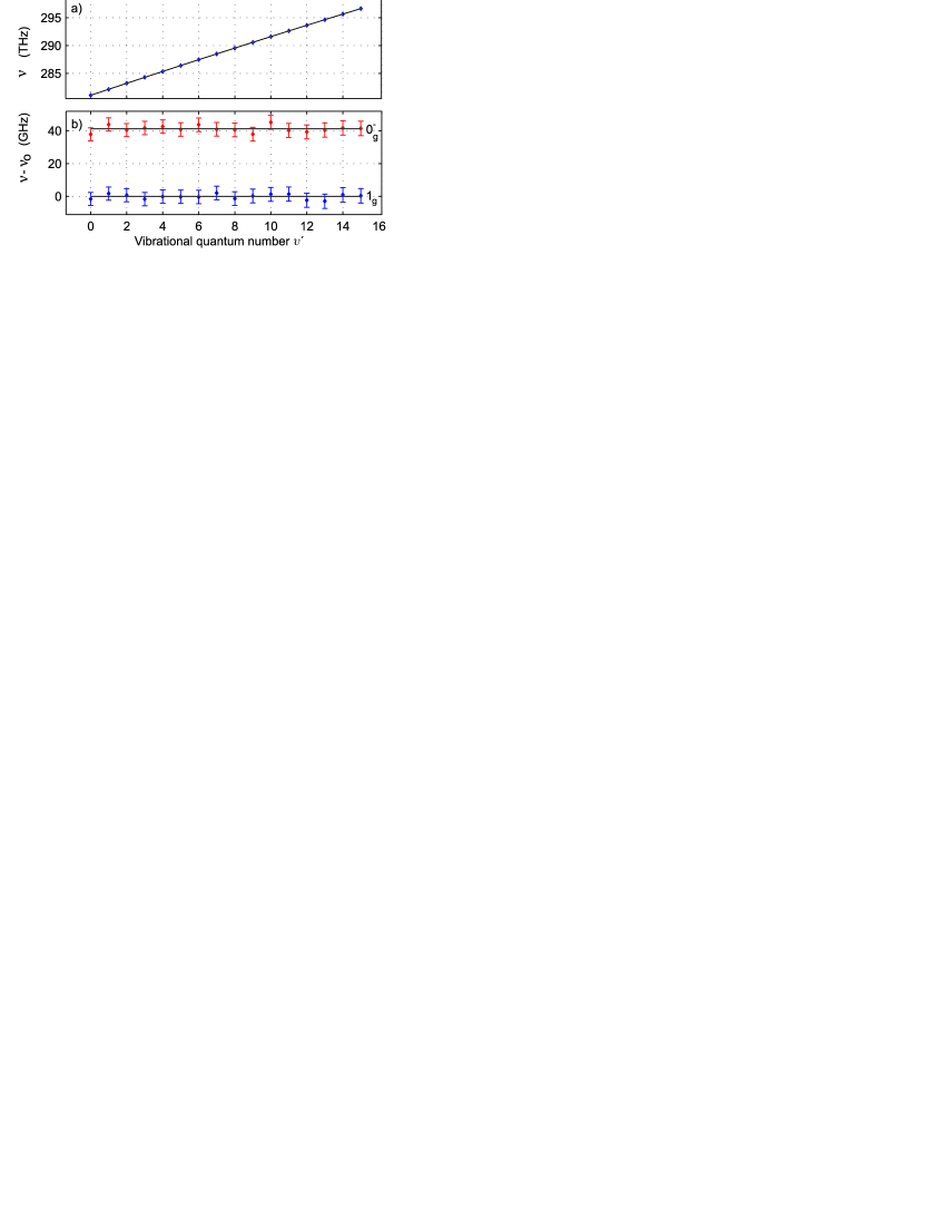
Figure 3: Vibrational ladder for the $(1)\,^{3}\Sigma_{g}^{+}$ state. a) Excitation frequencies $\nu$ of the vibrational states with quantum number $v^{\prime}$. The solid line is a quadratic fit to the data. b) Zoom into the vibrational levels which are split into a $0_{\textrm{g}}^{-}$ and a $1_{\textrm{g}}$ component. The spectra are measured at low resolution and high power. A frequency offset $\nu_{o}(v^{\prime})$ is subtracted from the excitation frequency $\nu$ for each data point. The offset $\nu_{o}(v^{\prime})$ is a quadratic fit to the $1_{\textrm{g}}$ data. Note the different energy scales of a) and b).

In a first set of experiments, we have mapped out the vibrational ladder of the $(1)\,^{3}\Sigma_{g}^{+}$ state from $v^{\prime}=0$ to $v^{\prime}=15$ at low resolution (Fig. 3a). We used the Ti:sapphire laser with an available power of a few hundred mW such that we only observed broad lines with a typical width of several GHz. The magnetic field was set to 986.8 G. The vibrational ground state of the $(1)\,^{3}\Sigma_{g}^{+}$ state has an excitation frequency of 281.1 THz with respect to $|i\rangle$, corresponding to a laser wavelength of 1067nm. The vibrational splitting between the two lowest levels, $v^{\prime}=0$ and $v^{\prime}=1$, is about 1.2 THz. The solid line in Fig. 3a is a quadratic fit in $v$ allowing for a slight anharmonicity in the vibrational ladder. The data lead to the same Morse potential as given by Mudrich et al. Mu10 . We find that each vibrational level is a doublet with a splitting of about 47 GHz lambdapar (see Fig. 3 b). The large error bars of several GHz reflect the crudeness of this first measurement where we do not resolve the substructure of each of the doublet components.

III.1 Splitting of the vibrational levels into $0_{\textrm{g}}^{-}$ and $1_{\textrm{g}}$ components

The 47 GHz splitting of the vibrational levels clearly cannot be explained by the rotational, hyperfine, or Zeeman interactions because they would be too small. Estimating the molecular hyperfine and Zeeman energies from those for ⁸⁷Rb atoms, we expect such contributions to be at most 14 GHz. It turns out that the large splitting comes from a strong effective spin-spin coupling of the electrons. Although there is direct spin-spin coupling, the main contribution is second order spin-orbit coupling, which is resonantly enhanced by the nearby $(1)^{1}\Pi_{g}$ state L06 . Experimentally, these two contributions cannot be separated. In its microscopic form, the effective spin-spin interaction Hamiltonian reads

$$H_{\text{ss}}=-C\frac{3(\mathbf{s}_{1}\cdot\mathbf{r}_{12})(\mathbf{s_{2}}\cdot\mathbf{r}_{12})-(\mathbf{s}_{1}\cdot\mathbf{s}_{2})\mathbf{r}_{12}^{2}}{r_{12}^{5}},$$ (1)

where $C$ is a constant, $\mathbf{s}_{1,2}$ are the electron spin operators, and $\mathbf{r}_{12}$ is the relative position vector of the two electrons. It can be shown Kramers1 ; Kramers2 that for $\Sigma$ states, $H_{\text{ss}}$ can be simplified to

$$H_{\text{ss}}=2\lambda[(\mathbf{n}\cdot\mathbf{S})^{2}-\mathbf{S}^{2}/3].$$ (2)

Here, $\lambda$ is effective molecular parameter for the spin-spin interaction which has to be determined for the studied vibrational level. $\mathbf{n}$ is the unit vector along the internuclear axis, and $\mathbf{S}$ is the total electronic spin operator with $\mathbf{S}=\mathbf{s}_{1}+\mathbf{s}_{2}$. Since the term $\mathbf{S}^{2}/3$ merely results in an overall offset, it will be ignored. Thus the spin-spin interaction takes the form

$$H_{\text{ss}}=2\lambda(\mathbf{n}\cdot\mathbf{S})^{2}.$$ (3)

A strong $H_{\text{ss}}$ couples the electronic spin to the internuclear axis, making its projection $\Sigma=0,1$ a good quantum number. Thus, for our $(1)\,^{3}\Sigma_{g}^{+}$ state $\Omega=\Lambda+\Sigma=\Sigma$ is also a good quantum number. Here $\Lambda$ and $\Omega$ are the projections of the total electronic orbital angular momentum $\mathbf{L}$ and the total angular momentum $\mathbf{J}=\mathbf{L}+\mathbf{R}+\mathbf{S}$ on the internuclear axis, where $\mathbf{R}$ is the rotational angular momentum of the nuclei. The eigenvalues of $H_{\text{ss}}$ are $2\lambda\Sigma^{2}$. This means that the splitting between the $\Omega=0$ and $\Omega=1$ states is 2$\lambda$. As will become clear later, the more deeply bound component of the observed doublet structure has $1_{\textrm{g}}$ character and the other one has $0_{\textrm{g}}^{-}$ character (Fig. 3 b), where we use Hund’s case (c) notation $|\Omega|_{g/u}$.

III.2 Spectra of the $0_{\textrm{g}}^{-}$ and $1_{\textrm{g}}$ states

The $0_{\textrm{g}}^{-}$ and $1_{\textrm{g}}$ states have a rich substructure which we are able to resolve by lowering the power of the laser to about 0.1 mW. Figures 4 and 5 show loss spectra for $1_{\textrm{g}}$ ($v^{\prime}=0,\,13$) and $0_{\textrm{g}}^{-}$ ($v^{\prime}=13$), respectively. While the $1_{\textrm{g}}$ manifold is spread out over 12 GHz, the $0_{\textrm{g}}^{-}$ manifold is narrower (3 GHz) and has fewer lines. The 12 observed lines of the $1_{\textrm{g}}$ manifold in Fig.  4 show no obvious pattern. The structure is the result of an interplay of rotational, hyperfine, and Zeeman interactions. It is one of the main goals of this work to understand this structure and to identify the individual lines.

A $1_{\textrm{g}}$ spectrum typically consists of roughly 300 points where each point corresponds to one production and measurement cycle. The lines that we observe vary markedly in width. This indicates a strong variation of the laser-induced coupling between $|v^{\prime}\rangle$ and $|i\rangle$. Spectra for different vibrational levels are similar (Fig. 4).

Compared to the typical step size of 40 MHz in Fig. 4, the 12 MHz natural linewidth of the molecular levels (given by twice the atomic linewidth) is relatively small. Thus, it is possible that some weak lines are not always detected, especially when they are located on the shoulder of a power-broadened line. We thus carried out a number of scans with various step sizes, laser powers, and pulse times, testing for consistency and checking theoretical predictions. For the $1_{\textrm{g}}$ spectra we found 18 lines in total (Section V).

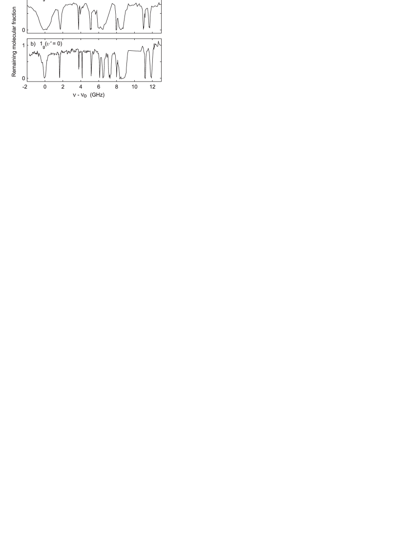
Figure 4: The $1_{\textrm{g}}$ spectra of two different vibrational levels at 986.8 G. For each spectrum, we subtract a frequency offset $\nu_{o}$ from the excitation frequency $\nu$ such that the most deeply bound line is situated at $0$ GHz. a) $v^{\prime}=13$, $\nu_{o}=294626.4$ GHz. b) $v^{\prime}=0$, $\nu_{o}=281068.2$ GHz. In these two scans, not all lines that we eventually observed are resolved.

Our $0_{\textrm{g}}^{-}$ spectrum is considerably simpler than the $1_{\textrm{g}}$ spectrum. There are 5 lines arranged in a doublet-like structure with a splitting of $\approx 2.5$ GHz (Fig. 5). This splitting is due to rotation of the molecule ,

$$H_{\text{rot}}=B_{v^{\prime}}\mathbf{R}^{2}/\hbar^{2},$$ (4)

where $B_{v^{\prime}}$ is the rotational constant and $\hbar$ is the reduced Planck constant. The hyperfine and Zeeman contributions are much weaker here. As we will show in section IV this can be explained due to the vanishing of the projections of total spin ${\bf S}$ and total orbital angular momentum ${\bf L}$ of the electrons on the internuclear axis. The rotational constant $B_{v^{\prime}}$ is

$$B_{v^{\prime}}=\frac{\hbar^{2}}{2\mu}\biggl{\langle}v^{\prime}\biggl{|}\frac{1}{r^{2}}\biggl{|}v^{\prime}\biggl{\rangle},$$ (5)

where $|v^{\prime}\rangle$ is the ket for the vibrational wave function, $r$ is the nuclear separation, and $\mu$ is the reduced mass. From previous investigations, Par01 ; L06 we expect $B_{v^{\prime}=13}/h=412$ MHz. Due to the weakness of the hyperfine and Zeeman interactions, the angular momentum ${\bf J}$ is conserved. Apart from an offset the rotational energy is then determined from Eq. (4) to be Lefebvre2004

$$E_{\text{rot}}=B_{v^{\prime}}\ J(J+1).$$ (6)

We observe the lines $J=0$ and $J=2$ separated by $6B_{v^{\prime}}/h\approx 2.5$ GHz (see Fig. 5). The rotational level $J=1$ is not accessible because total parity (under inversion of all electron and nuclear coordinates) has to change in the optical transition. The parity for the Feshbach molecule is $(-1)^{l}=+1$ while the parity of the states in the $0_{g}^{-}$ manifold of the $(1)\,^{3}\Sigma_{g}^{+}$ state is $(-1)^{J+1}$. The $J=2$ feature has a substructure of four lines which is due to residual hyperfine and Zeeman interaction. This substructure will be discussed in detail in section V hand in hand with the analysis of our theoretical model.

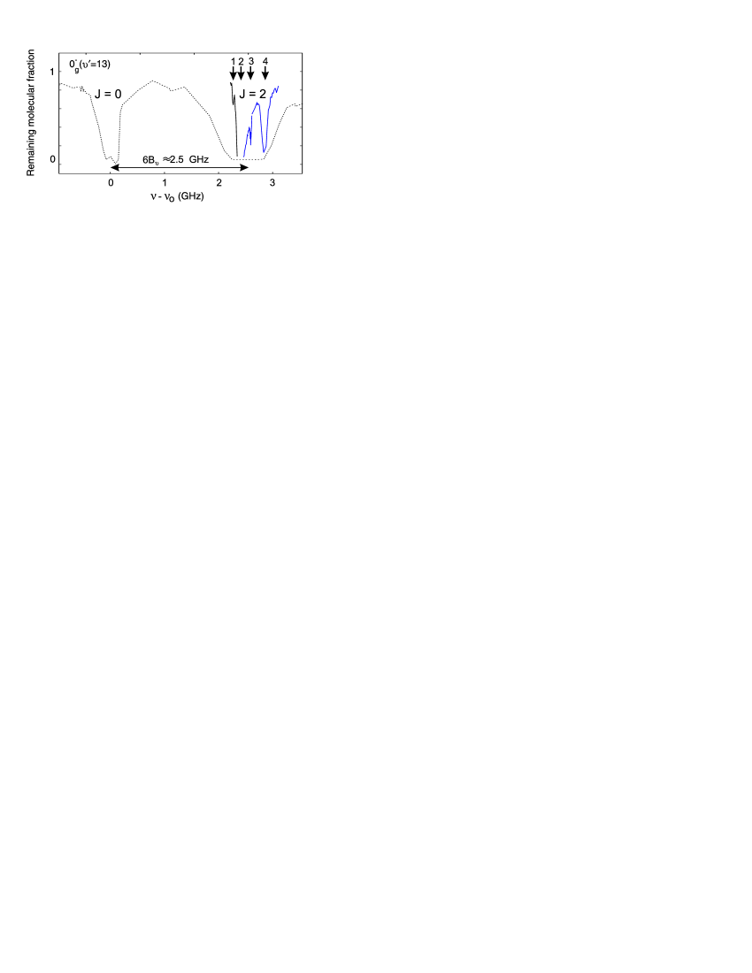
Figure 5: Scans of $0_{\textrm{g}}^{-}(v^{\prime}=13)$ lines in the $(1)\,^{3}\Sigma_{g}^{+}$ state at a magnetic field of 986.8 G. The dotted line corresponds to a laser power of 0.1 mW and a pulse duration of 200 ms while the solid line corresponds to a laser power of 0.1 mW and a 1 ms pulse duration. The frequency offset is $\nu_{o}=294671.0$ GHz. The line at $\nu-\nu_{o}$ = 0 GHz corresponds to $J=0$, while the 4 lines located around 2.5 GHz have $J=2$. Due to saturation these 4 lines are not resolved for the 200 ms pulse.

IV Effective Hamiltonian and evaluation of its parameters

In the following we present the diatomic model Hamiltonian which we use to describe the observed energy levels within the $v^{\prime}=13$ vibrational manifold. Spectra in other low lying vibrational manifolds are similar (Fig. 4), and can be described by the same Hamiltonian with slightly adjusted parameters. We can thus ignore electronic terms and vibrational motion. The Hamiltonian can then be written,

$$H=H_{\text{ss}}+H_{\text{rot}}+H_{\text{hf}}+H_{\text{Z}}+H_{\text{sr}}.$$ (7)

$H_{\text{ss}}=2\lambda(\mathbf{n}\cdot\mathbf{S})^{2}$ is the effective spin-spin operator given in Eq. (3) which, as previously discussed, leads to the large splitting into the $0_{\textrm{g}}^{-}$ and $1_{\textrm{g}}$ components. $H_{\text{rot}}=B_{v^{\prime}}\mathbf{R}^{2}/\hbar^{2}$ is the Hamiltonian for molecular rotation from Eq. (4). The terms for hyperfine interaction $H_{\text{hf}}$, Zeeman interaction $H_{\text{Z}}$, and finally spin-rotation interaction H${}_{\text{sr}}$ are described in the following. Since the goal in this article is to get a first understanding of the experimentally observed spectra, we will in general simplify the interaction and only take into account terms of leading order.

IV.1 The hyperfine interaction

A general ansatz for the hyperfine Hamiltonian in Hund’s case a) and b) is of the form Tow55

$$H_{\text{hf}}=a\ \Lambda\ \mathbf{I}\cdot\mathbf{n}+(b_{F}-{1\over 3}c)\ \mathbf{I}\cdot\mathbf{S}+c\ (\mathbf{I}\cdot\mathbf{n})\ (\mathbf{S}\cdot\mathbf{n}).$$ (8)

Here, $\mathbf{I}$ is the operator for the total nuclear spin. The first term describes the interaction of the electronic orbital angular momentum with the nuclear spin. However, since $\Lambda=0$, this term will not contribute. The Fermi contact parameter is $b_{F}$, while $c$ is called the anisotropic hyperfine parameter. For $\Sigma$-states, we expect $c\ll b_{F}$ (Tow55 , page 196). These two parameters could in principle be calculated ab-initio, but we have used them as free fit parameters. We note that the total nuclear spin I is a good quantum number for the given Hamiltonian.

IV.2 The Zeeman interaction

Because we carry out measurements at high magnetic fields, the Zeeman interaction plays an important role. The main contribution to the Zeeman interaction comes from the electrons while contributions from the nuclear spins and molecular rotation (as well as second order effects treated in Veseth ) are much smaller and are neglected here. Furthermore, since $\Lambda$ vanishes in the $(1)\,^{3}\Sigma_{g}^{+}$ state, the Zeeman interaction due to the total orbital angular momentum of the electrons, $\mu_{B}\mathbf{L}\cdot\mathbf{B}/\hbar$ is also negligible to first order. (Here, $\mu_{B}$ is the Bohr magneton). The only remaining term is

$$H_{Z}=\mu_{B}g_{S}\mathbf{S}\cdot\mathbf{B}/\hbar,$$ (9)

where $g_{S}$ is the electron g-factor. We note that there is no free fitting parameter in the Zeeman Hamiltonian for adjusting the model to the measured data. While the contribution from the Zeeman interaction will in general be large for the $1_{\textrm{g}}$ lines, it will be small for the $0_{\textrm{g}}^{-}$ lines because here the spin projection onto the internuclear axis $\Sigma=0$.

IV.3 The spin-rotation interaction

In principle, we could also include a spin-rotation interaction through the effective Hamiltonian

$$H_{\text{sr}}=\gamma_{v^{\prime}}\mathbf{N}\cdot\mathbf{S}.$$ (10)

where $\mathbf{N}=\mathbf{L}+\mathbf{R}$ and $\gamma_{v^{\prime}}$ is the spin-rotation coupling constant. However, since $\gamma_{v^{\prime}}$ is typically a small fraction of the rotational constant $B_{v^{\prime}}$ Lefebvre2004 , the spin-rotation interaction only represents an insignificant correction to the energy levels in the present system and is thus neglected.

IV.4 Fit procedure and evaluation of molecular parameters

According to our model Hamiltonian in Eq. (7) there are four adjustable parameters: the rotational constant $B_{v^{\prime}}$, the spin-spin splitting parameter $\lambda$, the Fermi-contact parameter $b_{F}$, and the anisotropic hyperfine parameter $c$. As discussed before in section III.2, the rotational constant $B_{v^{\prime}}$ should be close to 412 MHz based on previous work, and in agreement with our analysis of the $0_{\textrm{g}}^{-}$ spectrum in Fig. 5. The spin-spin parameter $\lambda$ is determined by the splitting of the $1_{\textrm{g}}$ and $0_{\textrm{g}}^{-}$ manifolds to be $2\lambda=47$ GHz. This leaves only $b_{F}$ and $c$ as completely free parameters. We determined all parameters from fits of the model to the experimental data using a nonlinear Levenberg-Marquardt method. For the calculations, the Hamiltonian in Eq. (7) is expressed in terms of matrix elements in a Hund’s case (a_α) basis, where the basis states are of the form

$$|\Lambda,S,\Sigma,I_{1},I_{2},\Omega_{I_{1}},\Omega_{I_{2}},F,\Omega_{F},M\rangle,$$ (11)

where $\Omega_{F}=\Lambda+\Sigma+\Omega_{I_{1}}+\Omega_{I_{2}}$ is the projection of the total angular momentum $F$ on the internuclear axis. $I_{1}$ = $I_{2}$ = 3/2 are the nuclear spins of the two nuclei and $\Omega_{I_{1}}$, $\Omega_{I_{2}}$ are their projections onto the internuclear axis. We note that the basis set (11) is chosen larger than necessary for our purpose. It can be conveniently used to investigate also Hamiltonians where the total nuclear spin $I$ ($\mathbf{I}=\mathbf{I_{1}}+\mathbf{I_{2}}$) might not be a good quantum number. For the analytical expressions of the matrix elements as a function of the quantum numbers of Eq. (11), we refer the reader to Marius09 . The Hamiltonian matrix is then numerically diagonalized to obtain the eigenvalues and eigenstates. Included in this calculation are all hyperfine states in the ${}^{3}\Sigma_{g}^{+}(v^{\prime}=13)$ electronic state with total angular momentum of up to $F=10$. Experimentally, we have only observed states with $F<7$. The parameters $b_{F}$ and $c$ are determined in terms of combination $b_{F}+{2\over 3}c$ and $b_{F}-{1\over 3}c$, which correspond to contributions diagonal and off-diagonal in $\Sigma$ and $\Omega_{I}=\Omega_{I_{1}}+\Omega_{I_{2}}$, respectively. The diagonal term can be directly read off from Eq. (8).

$$\begin{split}H_{\text{hf}}^{diag}&=(b_{F}-{1\over 3}c)\,\Omega_{I}\Sigma+c\,\Omega_{I}\Sigma\\ &=(b_{F}+{2\over 3}c)\,\Omega_{I}\Sigma.\end{split}$$ (12)

Our final analysis gives $B_{v^{\prime}}=412$ MHz, $2\lambda=47$ GHz and $b_{F}+{2\over 3}c=832$ MHz. We find, however, that $b_{F}-{1\over 3}c$ is not precisely determined in our analysis. Experimentally, the parameter $b_{F}-{1\over 3}c$ could, in principle, be best determined from the $0_{\textrm{g}}^{-}$ spectrum because the contribution to the hyperfine interaction is purely off-diagonal with respect to $\Sigma$. However, the energy levels depend only weakly on this parameter, and our measurements indicate a value between $(200-1000)$ MHz. Higher precision than that reached in our measurements is required in order to better estimate $(b_{F}-\frac{1}{3}c)$.

V Assignment of lines of the $0_{\textrm{g}}^{-}$ and $1_{\textrm{g}}$ spectra

With the help of our theoretical model, we can now identify the individual lines of the $0_{\textrm{g}}^{-}$ and $1_{\textrm{g}}$ spectra and understand the physical origin of the substructure of these spectra. Since the Feshbach molecules have total magnetic quantum number $M=2$, and since we use an optical $\pi$ transition, we only observe excited levels with $M=2$ and thus $F\geq 2$. From our discussion so far, we have the following good quantum numbers for our levels in the $(1)\,^{3}\Sigma_{g}^{+}$ state: $M=2,\Lambda=0;\Sigma=0,1;\Omega=0,1;S=1.$ Furthermore the total nuclear spin $I$ is a good quantum number in our Hamiltonian and as we will see in the next section can take the values $I=1,3$. At low magnetic field, $F$ is also a good quantum number. With these and the additional quantum number $J$, which (as we will show) is good for the $0_{\textrm{g}}^{-}$ states and becomes good for high-rotational $1_{\textrm{g}}$ states, we will be able to identify all lines.

V.1 $0_{\textrm{g}}^{-}$ Zeeman spectrum

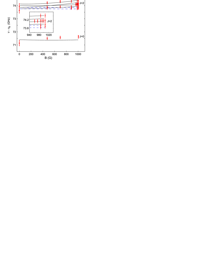
Figure 6: Zeeman diagram of the $0_{\textrm{g}}^{-}$ ($v^{\prime}=13$) state. An offset $\nu_{o}=294600$ GHz is subtracted from the excitation frequency $\nu$. The lines are calculations. Dashed lines indicate levels with $F>3$ that cannot be excited in our experiment at $B=0$ due to the selection rule on $\Delta F=0,\pm 1$. Table 1 gives the quantum numbers at 0 G and 1005.8 G. The inset is a zoom into the closely spaced lines around 1000 G.

Figure 6 shows experimentally observed energy levels for various magnetic field strengths along with the calculations (dashed and solid lines). The Zeeman effect is quite weak as levels shift no more than a couple hundred MHz over a range of 1000 G. This is consistent with our previous assertion in section IIIb that the Zeeman interaction ($\propto\mathbf{S}\cdot\mathbf{B}$) is small because the expectation value of the electron spin vanishes in any projection direction for a state with $\Sigma=0$. An identical argument holds for the hyperfine interaction in Eq. (8). The observed residual splitting of the lines in Fig. 6 is mainly due to second order contributions of the Zeeman and hyperfine interactions. The $0_{\textrm{g}}^{-}$ spectrum is dominated by the rotational splitting $B_{v^{\prime}}J(J+1)$. This overall trend is well described by the theory (Fig. 6). A slight discrepancy can be observed in the rotational splitting which seems to lie somewhat outside the experimental error bars. Note that at 0 G, experimental data are less accurate than for the other magnetic fields because of technical stability issues when we transfer the Feshbach molecules from 1007 G to low magnetic fields. Uncontrolled magnetic field drifts lead to fluctuations in the transfer efficiency across the avoided crossings from shot to shot, which made the measurements noisy.

We now study in detail the quantum numbers of the observed levels. Based on the exchange symmetry of the nuclei and other fundamental symmetries of the $(1)\,^{3}\Sigma_{g}^{+}$ state, one can show that the $J=0$ and $J=2$ levels have either total nuclear spin $I$ = 1 or 3. $\mathbf{J}$ and $\mathbf{I}$ couple to form the total angular momentum $\mathbf{F}$. For $J=0$ we obtain $F=1,3$, of which only $F=I=3$ is observed (the single line at $\approx\,$294671 GHz in Fig. 6). This is because we only detect levels that have a total magnetic quantum number $M=2$. Coupling $J=2$ with $I=1$ ($I=3$) results in states with $F=2,\,3$ ($F=2,\,3,\,4,\,5$), where we have omitted $F=1$ states, since again they cannot be observed. These six levels are plotted as lines in Fig. 6 and also listed in table 1 together with measured data. As can be read off from the expectation values in the table, for low magnetic fields the levels in the $0_{\textrm{g}}^{-}$ component are indeed well described by the quantum numbers $J,I,F.$ At 1000 G, $F$ is not good anymore.

In Fig. 6, two of the calculated lines are dashed. They correspond to $F=4,5$ which are not observable at 0G because of the selection rule $\Delta F=0,\pm 1$. For larger magnetic fields, the Zeeman interaction mixes states with different $F$ and the two levels that correlate with $F=4,5$ at 0 G become observable. As the magnetic field is increased, some lines cross. Because $I$ is exactly a good quantum number for our specific Hamiltonian $H$, crossings between levels with different $I$ quantum numbers are not avoided.

From Fig. 6 as well as from Table I, we see that apparently the two $I=1$ lines are not observed. Closed coupled-channel calculations privTiemann ; Str10 show that our Feshbach molecules only have a few percent $I=1$ character. The selection rule $\Delta I=0$ thus makes it clear that $I=1$ lines will be suppressed in the spectrum. We also know that the Feshbach state is a superposition of electronic singlet and triplet states. For $l=0$ one finds from symmetry arguments (inversion symmetry, rotational symmetry, exchange symmetry, reflection symmetry) that the triplet component has nuclear spin $I=1,3$ while the singlet component has $I=0,2$. Further, for $l=0$, the triplet component of the Feshbach state in the Hund’s case (c) basis has $J=1$, $\Omega=0$ while the singlet component has $J=0$. Only the electronic triplet part of the Feshbach state will contribute to the optical transition to the $(1)\,^{3}\Sigma_{g}^{+}$ $0_{\textrm{g}}^{-}$ state, fulfilling the standard Hund’s case (c) $\Omega=0\leftrightarrow\Omega=0$ selection rules $\Delta J=\pm 1,\Delta S=0,$ and $\Delta I=0$.

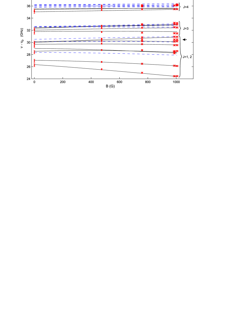
Figure 7: Zeeman diagram of the $1_{\textrm{g}}$ ($v^{\prime}=13$) state. An offset $\nu_{o}=294600\,\mathrm{GHz}$ is subtracted from the excitation frequency $\nu$. The lines are calculations. Dashed lines indicate levels with $F>3$ that can not be observed in our experiment at $B=0$ due to the selection rule $F=0,\pm 1$. The arrow points to an experimentally observed line that is not well described by the calculations. Table 2 gives the corresponding quantum numbers at 0 G.

	$B=0$ G				$B=1005.8$ G
$\langle J\rangle$	$\langle I\rangle$	$\langle F\rangle$	$\nu_{T}-\nu_{o}$	$\nu_{E}-\nu_{o}$	$\langle I\rangle$	$\langle F\rangle$	$\nu_{T}-\nu_{o}$	$\nu_{E}-\nu_{o}$
			(GHz)	(GHz)			(GHz)	(GHz)
0.0	3	3.0	71.44	71.14	3.0	3.0	71.42	71.63
2.0	3	5.0	73.84	n.o.	3.0	4.2	73.83	73.83
2.0	1	3.0	73.84	n.o.	3.0	3.7	73.95	73.92
2.0	1	2.0	73.92	n.o.	1.0	2.9	74.00	n.o.
2.0	3	4.0	73.94	n.o.	3.0	3.3	74.13	74.13
2.0	3	3.0	74.06	73.64	1.0	2.1	74.27	n.o.
2.0	3	2.0	74.17	73.95	3.0	2.8	74.42	74.40

Table 1: Calculated and measured $0_{\textrm{g}}^{-}$ $(v^{\prime}=13)$ excitation frequencies of the levels shown in Fig. 6 at 0 G and 1005.8 G. The offset from the excitation frequency $\nu$ is $\nu_{o}=294600$ GHz. The subscripts _T and _E denote theoretical and experimental values. The expectation values for quantum numbers $J$, $I$ and $F$ are also given. All levels have $S=1$, $\Sigma=0$, and $M=2$. Levels with $I=1$ are not observed (n.o.). The absolute accuracy for the measured line positions at $B=0$ and $1005.8$ G is about 200 MHz and 70 MHz, respectively. The accuracy for the relative positions of the lines, however, is in general higher, e.g. $\approx$20 MHz for the J = 2 lines at $B=1005.8$ G.

V.2 $1_{\textrm{g}}$ Zeeman spectrum

The experimental $1_{\textrm{g}}$ data at various magnetic fields together with the calculated energies are shown in Fig. 7. There is good agreement of the overall structure of the calculated levels and the observed data. Our calculations (Table 2) indicate that the angular momentum $J$ becomes a good quantum number for $J\geq 3$. Indeed, for $J\geq 3$, rotational lines belonging to different $J$ are energetically well separated and the rotational splitting starts to dominate the structure of the observed spectrum.

This can be understood as follows: A fast rotation of the molecular axis averages out the direction of the electron spin in the lab frame, because the electron spin is tightly coupled to the molecular axis ($\Sigma=1$). This leads to an effective decrease of the Zeeman interaction. Similarly, a fast rotation will prevent the nuclear spin $I$ from coupling to the molecular axis (and therefore to the electron spin), as it cannot follow fast enough in an adiabatic way. In fact, calculated expectation values for $\Omega_{I}$ (see Table 2) are close to 0 (typically $|\langle\Omega_{I}\rangle|<0.5$ for $J\geq 3$) indicating a strong averaging out. For slow rotations ($J\leq 2$), in contrast, the hyperfine and Zeeman interactions are of the same order as the rotational splitting. This leads to a relatively strong mixing between levels with $J=1$ and $J=2$. Note that for the $1_{\textrm{g}}$ manifold only levels with $J\geq 1$ exist since the projection $\Omega=1$.

The energetically lowest state has an expectation value $\langle|\Omega_{I}|\rangle=2.6$, which is close to its “ideal” value of 3 if the hyperfine interaction ($\propto\Omega_{I}\Sigma$) was dominant over the rotational and Zeeman interactions. We can now ask how large this hyperfine interaction is in the limit of smallest rotation, e.g. $J=1$. We can roughly estimate this by looking at Fig. 7. At $B=0$ the rotational splitting of the $J=1$ and $J=4$ levels has to be 18 $B_{v^{\prime}}$ = 7.2 GHz. The observed splitting between the barycenter of the $J=4$ levels and the lowest line at $\nu-\nu_{o}$ = 26.34 GHz is larger by about 2 GHz. This indicates that the hyperfine structure for $J\cong 1$ must be spread out over a range of roughly 4 GHz.

We now investigate the number of lines that can in principle be observed. For $J=4$ and $I=1,3$ we can form 9 states with $F\geq 2$. For $J=3$ we expect 8 states and for $J=1,2$ together we expect 10 states. These are the states which are listed in Table II. In contrast to the spectrum of $0_{\textrm{g}}^{-}$, we can observe levels with even as well as odd $J$, due to a two-fold degeneracy of each rotational level. One of the two levels has positive parity while the other one (that is observed in the experiment) has negative parity.

The fact that we observe levels with a rotation up to $J=4$ might at first be surprising, as we start from $J=1$ $\Omega=0$ in the Feshbach state and the selection rule is $\Delta J=0,\pm 1$. However, this simply shows that $J$ in the excited state is not a very good quantum number yet and the $J\approx 4$ levels have a $J=2$ contribution.

At zero magnetic field, the quantum number $F$ for the total angular momentum is good. At this field we cannot observe levels with $F>3$, due to the selection rule $\Delta F=0,\pm 1$. As in Fig. 6, these levels are drawn with dashed lines. Again, at larger magnetic fields levels with different $F$ mix, and as a consequence more levels can be reached. The curves in Fig. 7 also display level crossings. Crossings are in general avoided as long as the levels have the same $I$ quantum number. For our specific Hamiltonian $H$, where $I$ is exactly good quantum number, levels with different $I$ do not mix with each other.

The overall structure of the observed spectroscopic lines is well described with our model, which essentially only has a single free parameter, $b_{F}+{2\over 3}c$. However, we find significant deviations of up to a few 100 MHz (e.g. note the data point next to the small horizontal arrow in Fig. 7). Such deviations clearly lie outside our experimental uncertainty, especially since for these cases relative positions of neighboring lines are determined with a precision better than typically 30 MHz. On this level of accuracy, in general, we do not have good agreement with the theory.

In order to achieve better agreement, one must include terms in the theory that we have so far neglected. For example, the Zeeman term $\propto\mathbf{L}\cdot\mathbf{B}$ can contribute in second order. It could also contribute to first order if the projection $\Lambda$ is not completely vanishing due to mixing-in of a $\Lambda=1$ component from nearby states, e.g. via second order spin-orbit interaction. However, such investigations would also require more detailed measurements and must be left for future work.

$B=0$ G
$\langle J\rangle$	$\langle I\rangle$	$|\langle\Omega_{I}\rangle|$	$\langle F\rangle$	$\nu-\nu_{o}$ (GHz)
1.2	3.0	2.6	2.0	26.34
1.4	3.0	2.0	3.0	27.06
2.7	3.0	1.2	4.0	28.36
1.2	1.0	0.16	2.0	28.53
2.0	3.0	1.0	2.0	29.00
2.0	3.0	0.41	3.0	29.68
1.9	1.0	0.27	2.0	29.98
2.1	3.0	0.75	5.0	30.12
2.3	1.0	0.031	3.0	30.13
2.0	3.0	0.57	4.0	30.51
3.0	3.0	0.75	2.0	31.77
3.0	3.0	0.21	3.0	32.02
3.0	1.0	0.11	2.0	32.31
2.9	3.0	0.60	4.0	32.44
3.0	1.0	0.025	3.0	32.45
3.1	3.0	0.44	6.0	32.56
3.2	1.0	0.069	4.0	32.57
3.0	3.0	0.37	5.0	32.64
3.9	3.0	0.13	2.0	35.04
3.9	3.0	0.21	3.0	35.41
4.0	1.0	0.014	3.0	35.54
3.9	3.0	0.48	4.0	35.78
4.0	1.0	0.13	4.0	35.81
4.0	1.0	0.011	5.0	35.99
3.9	3.0	0.54	5.0	36.07
4.1	3.0	0.25	7.0	36.19
4.0	3.0	0.30	6.0	36.22

Table 2: Calculated $1_{\textrm{g}}$ $(v^{\prime}=13)$ excitation frequencies of the levels shown in Fig. 7 at 0 G. The offset from the excitation frequency $\nu$ is $\nu_{o}=294600$ GHz. The expectation values for quantum numbers $J$, $I$ and $F$ are also given. All levels have $S=1$, $\Sigma=1$, and $M=2$. Levels with $I=1$ are not observed.

VI Summary and Outlook

In this article we carry out high resolution molecular spectroscopy starting with an ultracold ensemble of ⁸⁷Rb₂ molecules. We are able to resolve the vibrational, rotational, hyperfine and Zeeman structure of deeply bound states ($v^{\prime}<15$) of the excited $(1)\,^{3}\Sigma_{g}^{+}$ state. The accuracy of the measured lines is about 60 MHz, however, the relative position of the lines with respect to each other is often determined much better and its accuracy reaches 20 MHz. The dominating feature of the observed spectra is the splitting of the vibrational levels into a $1_{\textrm{g}}$ and a $0_{\textrm{g}}^{-}$ component which can be understood as a strong effective spin-spin coupling of the electrons. We obtain a good understanding of the level structure to first order with a relatively simple effective model that only takes into account the most important terms of the Hamiltonian. In brief, the level structure for the $0_{\textrm{g}}^{-}$ line is mainly determined by the vanishing spin component $\Sigma=0$, which leads to a very small hyperfine and Zeeman structure and a good quantum number $J$. In contrast, for the $1_{\textrm{g}}$ line, the hyperfine and Zeeman interactions are large for small rotations, but then are averaged out at larger rotations such that the rotational splitting according to $J(J+1)$ again determines the spectrum. Despite the overall understanding of the level structure, we still observe systematic deviations between experiment and theory on the order of a few 100 MHz, which should disappear in a more refined model. We find from our data that the anisotropic part of the hyperfine interaction could essentially not be determined. In order to do this, the experimental data of the $0_{\textrm{g}}^{-}$ line will have to be measured with higher precision in the future.

It would be interesting to see whether the determined fit parameters for $\lambda$ (effective spin-spin interaction) and for the hyperfine contact interaction can be deduced from ab-initio calculations and the known atomic properties. Besides gaining a better insight into the level structure of the so-far relatively unexplored $(1)\,^{3}\Sigma_{g}^{+}$ state, this work will be helpful for future cold molecule experiments where the deeply bound molecules need to be prepared with high efficiency in various well defined quantum states of the $a\,^{3}\Sigma_{u}^{+}$ state. Levels in the $(1)\,^{3}\Sigma_{g}^{+}$ state may then serve as an intermediate state-selective step in a two-photon optical transfer scheme from Feshbach molecules La08 .

- (1) K. M. Jones, E. Tiesinga, P. D. Lett, and P. S. Julienne, Rev. Mod. Phys. 78, 483 (2006).
- (2) T. Köhler, K. Goral, and P. S. Julienne, Rev. Mod. Phys. 78, 1311 (2006).
- (3) J. Weiner, V. S. Bagnato, S. Zilio and P. S. Julienne, Rev. Mod. Phys. 71, 1 (1999).
- (4) J. M. Sage, S. Sainis, T. Bergeman, D. DeMille, Phys. Rev. Lett. 94, 203001 (2005).
- (5) F. Lang, K. Winkler, C. Strauss, R. Grimm, and J. Hecker Denschlag, Phys. Rev Lett. 101, 133005 (2008).
- (6) J. G. Danzl, E. Haller, M. Gustavsson, M. J. Mark, R. Hart, N. Bouloufa, O. Dulieu, H. Ritsch, and H.-C. Nägerl, Science 321, 1062 (2008).
- (7) K.-K. Ni, S. Ospelkaus, M. H. G. de Miranda, A. Pe’er, B. Neyenhuis, J. J. Zirbel, S. Kotochigova, P. S. Julienne, D. S. Jin, and J. Ye, Science 322, 5899 (2008).
- (8) M. Viteau, A. Chotia, M. Allegrini, N. Bouloufa, O. Dulieu, D. Comparat, and P. Pillet, Science 321, 232 (2008).
- (9) J. Deiglmayr, A. Grochola, M. Repp, K. Mörtlbauer, C. Glück, J. Lange, O. Dulieu, R. Wester, and M. Weidemüller, Phys. Rev Lett. 101, 133004 (2008).
- (10) S. Ospelkaus, K.-K. Ni, G. Quéméner, B. Neyenhuis, D. Wang, M. H. G. de Miranda, J. L. Bohn, J. Ye, and D. S. Jin, Phys. Rev Lett. 104, 030402 (2010).
- (11) S. Ospelkaus, K.-K. Ni, D. Wang, M. H. G. de Miranda, B. Neyenhuis, G. Quéméner, P. S. Julienne, J. L. Bohn, D. S. Jin, and J. Ye, Science 327, 853 (2010).
- (12) K.-K. Ni, S. Ospelkaus, D. Wang, G. Quéméner, B. Neyenhuis, M. H. G. de Miranda, J. L. Bohn, J. Ye and D. S. Jin, Nature 464, 1324 (2010).
- (13) P. Staanum, S. D. Kraft, J. Lange, R. Wester, and Matthias Weidemüller, Phys. Rev. Lett. 96, 023201 (2006).
- (14) R. V. Krems, Int. Rev. Phys. Chem. 24, 99 (2005).
- (15) R. V. Krems, Phys. Chem. Chem. Phys. 10, 4079 (2008).
- (16) C. Chin, V. V. Flambaum, and M. G. Kozlov, New J. Phys. 11, 055048 (2009).
- (17) T. Zelevinsky, S. Kotochigova and J. Ye, Phys. Rev. Lett. 100, 043201 (2008).
- (18) D. DeMille, S. Sainis, J. Sage, T. Bergeman, S. Kotochigova, and E. Tiesinga, Phys. Rev. Lett. 100, 043202 (2008).
- (19) J. Bai, E. H. Ahmed, B. Beser, Y. Guan, S. Kotochigova, A. M. Lyyra, S. Ashman, C. M. Wolfe, J. Huennekens, Feng Xie, Dan Li, Li Li, M. Tamanis, R. Ferber, A. Drozdova, E. Pazyuk, A. V. Stolyarov, J. G. Danzl, H.-C. N gerl, N. Bouloufa, O. Dulieu, C. Amiot, H. Salami, and T. Bergeman, Phys. Rev. A 83, 032514 (2011).
- (20) Tom Bergeman, private communication.
- (21) K. Winkler, F. Lang, G. Thalhammer, P. v. d. Straten, R. Grimm, and J. Hecker Denschlag, Phys. Rev. Lett. 98, 043201 (2007).
- (22) C. Strauss, T. Takekoshi, F. Lang, K. Winkler, R. Grimm, E. Tiemann, and J. Hecker Denschlag, Phys Rev A 82, 052514 (2010).
- (23) J. Lozeille, A. Fioretti, C. Gabbanini, Y. Huang, H. K. Pechkis, D. Wang, P. L. Gould, E. E. Eyler, W. C. Stwalley, M. Aymar and O. Dulieu, Eur. Phys. J. D. 39, 261 (2006).
- (24) M. Mudrich, Ph. Heister, T. Hippler, Ch. Giese, O. Dulieu, and F. Stienkemeier, Rev. Rev. A 80, 042512 (2009).
- (25) G. Thalhammer, K. Winkler, F. Lang, S. Schmid, R. Grimm, and J. Hecker Denschlag, Phys. Rev. Lett. 96, 050402 (2006).
- (26) W. Ketterle, D. S. Durfee, and D. M. Stamper-Kurn, Making, probing and understanding Bose-Einstein condensates, in: M. Inguscio, S. Stringari, and C. E. Wieman (Eds.), Proceedings of the International School of Physics - Enrico Fermi, 67, IOS Press, 1999.
- (27) F. Lang, P.v.d. Straten, B. Brandstätter, G. Thalhammer, K. Winkler, P. S. Julienne, R. Grimm, and J. Hecker Denschlag, Nature Phys. 4, 223 (2008).
- (28) T. Volz, S. Dürr, S. Ernst, A. Marte, and G. Rempe, Phys. Rev. A 68, 010702 (2003).
- (29) In general, we define expectation values for the quantum numbers of an operator as , where are the eigenvalues of the operator, are corresponding normalized eigenvectors, and is the state.
- (30) S. J. Park, S. W. Suh, Y. S. Lee, and G.-H. Jeungy, J. Mol. Spectrosc. 207, 129 (2001).
- (31) G. Herzberg, Molecular Spectra and molecular structure - Vol I, D. Van Nostrand company (1950).
- (32) C. H. Townes, and A. L. Schawlow, Microwave Spectroscopy, McGraw-Hill Book Company (1955).
- (33) In order to obtain the splitting value of 47 GHz we have taken into account the full substructure of the and lines and our effective Hamilton model. If we ignore the substructure and simply use the observed barycenters of the and lines we obtain a splitting of about 42 GHz.
- (34) H. A. Kramers, Zeitschrift fuer Physik 53, 422 (1929).
- (35) H. A. Kramers, Zeitschrift fuer Physik 53, 429 (1929).
- (36) L. Veseth, J. Mol. Spectrosc. 63, 180-192 (1976).
- (37) H. Lefebvre-Brion and R. W. Field, The Spectra and Dynamics of Diatomic Molecules, Academic Press, Revised Edition (2002).
- (38) Eberhard Tiemann, private communication.
- (39) M. Lysebo and L. Veseth, Phys. Rev A 79, 062704 (2009).