Complex Time Evolution of Open Quantum Systems.
C. N. Gagatsos, A. I. Karanikas and G. I. Kordas
University of Athens, Physics Department
Nuclear & Particle Physics Section
Panepistimiopolis, Ilissia GR 15771, Athens, Greece

Abstract

We combine, in a single set-up, the complex time parametrization in path integration, and the closed time formalism of non-equilibrium field theories to produce a compact representation of the time evolution of the reduced density matrix. In this framework we introduce a cluster-type expansion that facilitates perturbative and non-petrurbative calculations in the realm of open quantum systems. The technical details of some very simple examples are discussed.

PACS: 03.65.-w, 03.65.Yz

1. Introduction.

In recent years there has been increasing interest in the consistent description of the dynamics of open quantum systems [1, 2, 3, 4, 5]. Quantum decoherence and dissipation are very important phenomena in many different areas of physics. A non-exhaustive list includes problems from quantum optics to many body and field-theoretical systems. Dissipative processes play a basic role in the quantum theory of lasers and photon detection, and they are equally important in nuclear fission and the deep inelastic collisions of heavy ions. More recently, the influence of the environment on a quantum system emerged as an issue of crucial importance, not only due to its fundamental implications, but also due to its practical applications in quantum information theory [8, 9, 10]. In fact, during the last decade, many new discoveries regarding the physics of open quantum systems were made. Primary examples of a promising progress can be found in the rapidly developing field of quantum optics and the connected continuous variable systems in quantum computation [12, 13].

Theoretical studies of decoherence and dissipation in quantum mechanics are centered on the time evolution of the reduced density matrix of a system embedded in a specific environment. The basic tools for studying the reduced dynamics are either effective equations of motion, where the dynamics of the environment are eliminated, such as the Lindblad master equation [6, 7], or the influence functional technique introduced by Feynman and Vernon [14]. The latter is based on the path integral approach, and was used by A. Caldeira and A. Leggett [15] in the study of the quantum Brownian motion more than twenty years ago. In most cases, however, neither the Lindblad equation nor the influence functional can be exactly evaluated, since the interaction between the system and the environment is too complicated. In fact, the simulation of the environment by a system whose degrees of freedom are treated as random variables following a more or less simple distribution, is a rather common practice. Therefore, one usually relies on some simple, specific system-environment models: a harmonic oscillator or a two-level quantum mechanical system embedded in a (thermal) bath of other harmonic oscillators or other spin systems. In the present work we aim to introduce and investigate calculational tools capable of exploring the behavior of an open system in interaction with a specific quantum environment. To be precise, we investigate the possibility to extend the calculational capability of the Feynman-Vernon path integral approach by adopting and combining definite functional methodological tools already known from different research fields. The first such tool is a combination of the well-known “closed (real) time formalism” [18] with the (equally well-known) imaginary time formulation [2] in the context of path integration. The compound result, called “closed complex time formalism” (or CCT ), enables us to isolate, in a simple and compact expression, the influence of the environment on the evolution of the system. It is well known that, in general, the integration of the environmental degrees of freedom does not produce a local “effective action” that controls the dynamics of the sub-system. The so-called Feynman-Vernon action, which incorporates the influence of the environment, is a highly non-local object: it is non-local in time and in space. The proposed CCT technique has a well-defined result: it produces an influence functional that can be viewed as an action local in space. In this action the paths are defined on the complex plane and they are parametrized with the help of a “time” running on a specific contour of the complex plane. The interest in such formalism is not “theoretical” but practical: one hopes to transfer the existent richness of perturbative and non-perturbative path integral techniques into the realm of open quantum systems.

Our second suggestion, strongly related to the first one, is the application of the so-called “cluster expansion” in the CCT context. The foundation of the application of this very powerful technique, of course, lies in the spatial locality -on the complex plane- of the influence functional. The cluster -or cumulant- expansion results to an expression that can be viewed as the “effective action” that governs the dynamics of the system after the elimination of the environmental degrees of freedom. However, in general, the cluster expansion produces an infinite series that contains all the orders of the environmental connected correlators and, if it is to be useful, some kind of truncation is necessary. As a first step in this direction, we consider the case in which the environmental correlators are of very fast decrease. Our formalism allows us to prove quite generally and without any reference to a specific model, that the two-point environmental correlator (which is the most important in our approximation scheme) has all the properties that can lead the subsystem to decoherence and dissipation. It is worth noting that our proposal can be extended to systems with an infinite number of degrees of freedom, such as the electromagnetic field interacting with matter or other field-theoretical systems.

The remainder of the paper is organized as follows: In Section 2 we present the details of the complex time formalism in the context of the path integral formulation of the Feynman-Vernon influence functional, and we discuss the assumptions under which the aforementioned formalism is applicable. In Section 3 we apply the cluster expansion in the framework of the CCT formalism, and we discuss the emergence of some quite general and very important properties of the influence functional. In subsection 3.1 we provide a specific example of an environment which is just a simple harmonic oscillator (or a collection of non-interacting harmonic oscillators). In Section 4 we consider the case of an environment in which the correlations decay very fast after some characteristic time interval. This stochastic behavior truncates the cluster series, enabling explicit calculations pertaining to the open system per se. As a first step in this direction, in the same section we calculate the entanglement entropy of a simple harmonic oscillator. Finally, in Appendix A we present the details of the calculation needed for deriving the results appearing in section 4.

2. Time Evolution and the Closed Complex Time Formalism.

The best way to interpret the usefulness of the closed complex time methodology (CCT from now on) is the examination of the time evolution of the reduced (environment averaged) density matrix of an open quantum central system (s from now on), which interacts linearly with its environment (e from now on). Adopting the usual starting point we assume that the total Hamiltonian can be written as the sum of two parts that refer to the system and the environment respectively, and a third part describing their interaction:

$$\hat{H}=\hat{H}_{s}+\hat{H}_{e}+\hat{H}_{I}$$ (1)

The total system evolves in time unitarily and, consequently, the reduced density matrix changes in time according to the equation:

$$\hat{\rho}^{R}(t,t_{0})=tr_{e}[\hat{U}(t,t_{0})\hat{\rho}(t_{0})\hat{U}^{{\dagger}}(t,t_{0})]$$ (2)

The dynamical content of the last expression is incorporated into a time evolution operator that contains the degrees of freedom of the whole system:

$$\hat{U}(t,t_{0})=\hat{T}\exp\left\{-\frac{i}{\hbar}\int_{t_{0}}^{t}dt^{\prime}\hat{H}(t^{\prime})\right\}$$ (3)

In the last expression we have taken into account a possible time dependence of the Hamiltonian. Physically we understand such dependence in various ways; for example, we can imagine that, after a sudden quench, the coupling between the central system and its environment changes to a different value, remaining constant henceforth. A case of physical interest arises when the coupling changes continuously and slowly enough to consider the evolution of the whole system as adiabatic. Another example is the well-studied case of an external time dependent field coupled linearly to the central system. In any case the operator $\hat{T}$ takes care of the needed time ordering. For now let us assume that, at the initial time $t_{0}$ (for the sake of convenience, in what follows we shall assume that $t_{0}=0$), the total system is prepared in a pure disentangled state

$$|\psi\rangle=|\psi_{s}\rangle\otimes|\psi_{e}\rangle.$$ (4)

Consequently, we can rewrite the reduced density matrix in the form:

$$\hat{\rho}^{R}(t)=tr_{e}[\hat{U}(t)\hat{\rho}_{s}(0)\otimes\hat{\rho}_{e}(0)\hat{U}^{{\dagger}}(t)]$$ (5)

Denoting by $\vec{x}$ and $\vec{q}$ the coordinates of the central system and the environment respectively, and by $\vec{X}=(x_{1},...,x_{D};q_{1},...,q_{D})$ the coordinates of the whole system collectively, eq. (5) can be written in the well known form:

$$\rho^{R}_{\vec{x}^{\prime}\vec{x}}(t)=\int d^{D}x^{\prime\prime}\int d^{D}x^{\prime\prime\prime}\rho^{s}_{\vec{x}^{\prime\prime}\vec{x}^{\prime\prime\prime}}(0)J(\vec{x},\vec{x}^{\prime},\vec{x}^{\prime\prime},\vec{x}^{\prime\prime\prime};t)$$ (6)

where the propagating kernel can be read from the expression:

$$J(\vec{x},\vec{x}^{\prime},\vec{x}^{\prime\prime},\vec{x}^{\prime\prime\prime};t)\equiv\int d^{D}q\int d^{D}q^{\prime\prime}\int d^{D}q^{\prime\prime\prime}\rho^{e}_{\vec{q}^{\prime\prime}\vec{q}^{\prime\prime\prime}}(0)\langle\vec{x}^{\prime},\vec{q}|\hat{U}(t)|\vec{X}^{\prime\prime}\rangle\langle\vec{X}^{\prime\prime\prime}|\hat{U}^{{\dagger}}(t)|\vec{X}\rangle.$$ (7)

Our next assumption is that the environment is initially in its ground state:

$$|\psi_{e}\rangle=|0_{e}\rangle$$ (8)

Then, it can easily be shown that [19]:

$$\rho^{e}_{\vec{q}^{\prime\prime},\vec{q}^{\prime\prime\prime}}(0)=\langle\vec{q}^{\prime\prime}|0_{e}\rangle\langle 0_{e}|\vec{q}^{\prime\prime\prime}\rangle=$$

$$=\frac{1}{Z_{e}}\mathop{\int\mathcal{D}\vec{q}^{(3)}}\limits_{\vec{q}^{(3)}(-0)=\vec{q}^{\prime\prime}}\mathop{\int\mathcal{D}\vec{q}^{(2)}}\limits_{\vec{q}^{(2)}(+0)=\vec{q}^{\prime\prime}}\exp\Bigg{\{}-\frac{1}{\hbar}\int_{-\infty}^{-0}d\tau\mathcal{L}_{e}^{(E)}[q^{(3)}]-\frac{1}{\hbar}\int_{0}^{\infty}d\tau\mathcal{L}_{e}^{(E)}[q^{(2)}]\Bigg{\}}$$ (9)

In the last expression we denoted by $\mathcal{L}_{e}^{(E)}$ the Euclidean version of the Lagrangian describing the dynamics of the environment. The origin of eq.(9) can be traced back to the propagator:

$$G_{e}(\vec{q}^{\prime\prime},t^{\prime};\vec{q}^{\prime\prime\prime},t)=\sum_{n_{e}}\langle\vec{q}^{\prime\prime}|\exp\left\{-\frac{i}{\hbar}(t^{\prime}-t)\hat{H}_{e}\right\}|n_{e}\rangle\langle n_{e}|\vec{q}^{\prime\prime\prime}\rangle=$$

$$=\sum_{n_{e}}\exp\left\{-\frac{i}{\hbar}(t^{\prime}-t)E_{n_{e}}\right\}\phi_{n_{e}}(\vec{q}^{\prime\prime})\phi_{n_{e}}^{\ast}(\vec{q}^{\prime\prime\prime})$$ (10)

Introducing the Euclidean time $\tau=it$, taking the limits, $\tau=-T_{E}$, $\tau^{\prime}=0$, $T_{E}\rightarrow\infty$ and assuming that the ground state is unique one can easily deduce that

$$G_{e}(\vec{q}^{\prime\prime},0;\vec{q}^{\prime\prime\prime},-T_{E})=\langle\vec{q}^{\prime\prime}|0_{e}\rangle\langle 0_{e}|\vec{q}^{\prime\prime\prime}\rangle e^{-T_{E}E_{0_{e}}/\hbar}\Bigg{[}1+\mathcal{O}\left(e^{-T_{E}(E_{n_{e}}-E_{0_{e}})/\hbar}\right)\Bigg{]}$$ (11)

and, consequently the ground state wave function can be determined through an integration of the Euclidean propagator:

$$\langle\vec{q}^{\prime\prime}|0_{e}\rangle\sim\int d\vec{q}^{\prime\prime\prime}G_{e}(\vec{q}^{\prime\prime},0;\vec{q}^{\prime\prime\prime},-\infty)=\mathop{\int\mathcal{D}\vec{q}}\limits_{\vec{q}(-0)=\vec{q}^{\prime\prime}}\exp\left\{-\frac{1}{\hbar}\int_{-\infty}^{-0}d\tau\mathcal{L}_{e}^{(E)}[q]\right\}$$ (12)

The above relation is the basis of eq.(9) in which we also introduced the normalization factor

$$Z_{e}=\mathop{\int\mathcal{D}\vec{q}}\limits_{\vec{q}(-\infty)=\vec{q}(\infty)}\exp\left\{-\frac{1}{\hbar}\int_{-\infty}^{+\infty}d\tau\mathcal{L}_{e}^{(E)}[q]\right\}$$ (13)

ensuring that $tr_{e}[\hat{\rho}_{e}(0)]=1$ and we used a numbering convenient for our future considerations. To proceed further we write:

$$\langle\vec{x}^{\prime},\vec{q}|\hat{U}(t)|\vec{X}^{\prime\prime}\rangle=\mathop{\int\mathcal{D}\vec{X}^{(4)}}\limits_{\vec{x}^{(4)}(0)=\vec{x}^{\prime\prime}}^{\vec{x}^{(4)}(t)=\vec{x}^{\prime}}\delta[\vec{q}^{(4)}(t)-\vec{q}]\delta[\vec{q}^{(4)}(0)-\vec{q}^{\prime\prime}]\exp\Bigg{\{}\frac{i}{\hbar}\int_{0}^{t}dt^{\prime}\mathcal{L}_{e}[\vec{X}^{(4)}]\Bigg{\}}$$ (14)

and

$$\langle\vec{X}^{\prime\prime\prime}|\hat{U}(t)|\vec{X}\rangle=\mathop{\int\mathcal{D}\vec{X}^{(1)}}\limits_{\vec{x}^{(1)}(0)=\vec{x}^{\prime\prime\prime}}^{\vec{x}^{(1)}(t)=\vec{x}}\delta[\vec{q}^{(1)}(t)-\vec{q}]\delta[\vec{q}^{(4)}(0)-\vec{q}^{\prime\prime\prime}]\exp\left\{\frac{i}{\hbar}\int_{t}^{0}dt^{\prime}\mathcal{L}_{e}[\vec{X}^{(1)}]\right\}.$$ (15)

Inserting eqs.(9), (14) and (15) in expression (7) we find:

$$J(\vec{x},\vec{x}^{\prime},\vec{x}^{\prime\prime},\vec{x}^{\prime\prime\prime};t)=$$

$$=\frac{1}{Z_{e}}\mathop{\int\mathcal{D}\vec{x}^{(1)}}\limits_{\vec{x}^{(1)}(0)=\vec{x}^{\prime\prime\prime}}^{\vec{x}^{(1)}(t)=\vec{x}}\mathop{\int\mathcal{D}\vec{x}^{(4)}}\limits_{\vec{x}^{(4)}(0)=\vec{x}^{\prime\prime}}^{\vec{x}^{(4)}(t)=\vec{x}^{\prime}}\exp\Bigg{\{}\frac{i}{\hbar}\int_{0}^{t}dt^{\prime}\mathcal{L}_{s}[x^{(4)}]+\frac{i}{\hbar}\int_{t}^{0}dt^{\prime}\mathcal{L}_{s}[x^{(1)}]\Bigg{\}}\mathcal{F}[x^{(4)},x^{(1)};t].$$ (16)

The last factor in the above equation defines the well-known Feynman-Vernon functional [14] which incorporates the influence of the environment to the time evolution of the system:

$$\mathcal{F}[x^{(4)},x^{(1)};t]=\left(\prod_{i=1}^{4}\int\mathcal{D}\vec{q}^{(i)}\right)\delta[\vec{q}^{(4)}(0)-\vec{q}^{(3)}(-0)]\delta[\vec{q}^{(4)}(t)-\vec{q}^{(1)}(t)]\delta[\vec{q}^{(2)}(+0)-\vec{q}^{(1)}(0)]\times$$

$$\times\exp\Bigg{\{}\frac{i}{\hbar}\int_{0}^{t}dt^{\prime}\mathcal{L}_{e+I}[\vec{X}^{(4)}]-\frac{1}{\hbar}\int_{-\infty}^{-0}d\tau\mathcal{L}_{e}^{(E)}[q^{(3)}]-\frac{1}{\hbar}\int_{0}^{\infty}d\tau\mathcal{L}_{e}^{(E)}[q^{(2)}]+\frac{i}{\hbar}\int_{t}^{0}dt^{\prime}\mathcal{L}_{e+I}[\vec{X}^{(1)}]\Bigg{\}}$$ (17)

Up to this point the only difference of the last result from the usual line of thinking [1, 2, 3, 4] is that we consider the environment not as a heat bath in thermal equilibrium but as a quantum system -probably a very complicated one- in its ground state.

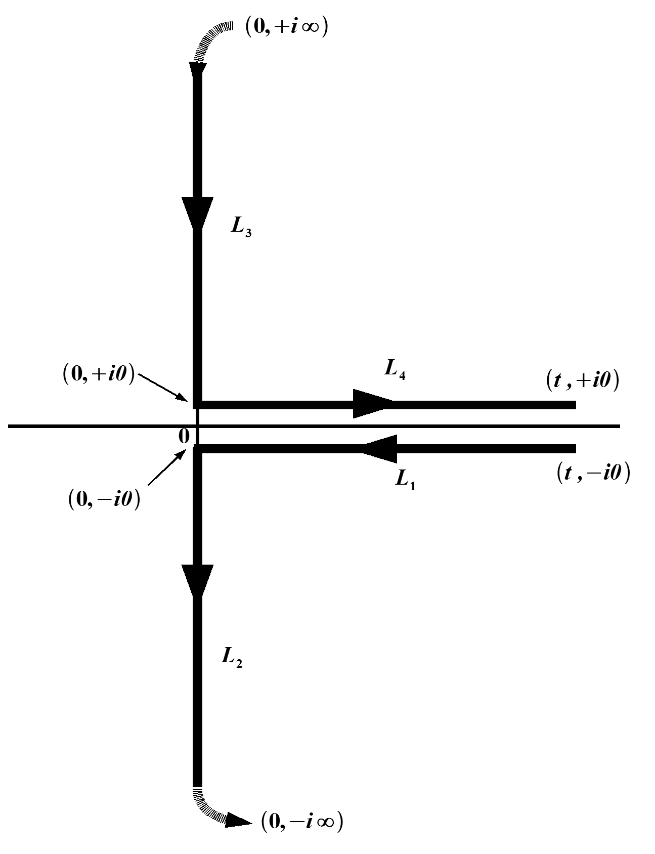
Figure 1: The Contour C

The expression for the influence functional can now be considerably simplified if we introduce the complex variable $z$ defined on the contour $C$ shown in Fig. 1. This contour consists of 4 different straight lines: The first line $L_{1}$ goes parallel to the real axis from the point $\textit{z}=t-i0$ to point $\textit{z}=0-i0$. The second line $L_{2}$ begins from the point $\textit{z}=0-i0$ and, following a path along the imaginary axis, goes to $\textit{z}=0-i\infty$. The line $L_{3}$ traces a path along the imaginary axis and joins the points $\textit{z}=0+i\infty$ and $\textit{z}=0+i0$. The last part of the contour is the straight line $L_{4}$ : It goes parallel to the real axis from the point $\textit{z}=0+i0$ to point $\textit{z}=t+i0$. It is now easy to be proved that the “action” in the influence functional (17) can be written as follows:

$$\tilde{S}=\int_{C}d\textit{z}\big{\{}\mathcal{L}_{e}[q_{c}]+\mathcal{L}_{I}[q_{c},x_{c}]\big{\}}=\int_{C}d\textit{z}\big{\{}\mathcal{L}_{e}[q_{c}]+g_{c}q_{c}x_{c}\big{\}}.$$ (18)

The notation in the last equation is defined as follows: Along the lines $L_{i}$, $i=1,\ldots,4$ , we have written $(\vec{x}_{L_{i}},\vec{q}_{L_{i}})=(\vec{x}^{(i)},\vec{q}^{(i)})$ and we have introduced a contour dependent coupling $g_{c}$ with $g_{L_{1}}=g_{L_{4}}=g$ and $g_{L_{2}}=g_{L_{3}}=0$. In expression (18) we have explicitly assumed that the interaction between the system and the environment is linear and has the minimal coupling $L_{I}=gxq$. In what follows we shall also assume that the coupling $g$ is time independent, but our considerations can easily be generalized to a time dependent coupling.

To confirm that eq.(18) does indeed represent the action in the influence functional, let us note that along the lines $L_{1}$ and $L_{4}$ we can write $\textit{z}=t^{\prime}-i0$, and consequently:

$$\int_{L_{1}}d\textit{z}\big{\{}\mathcal{L}_{e}[q_{L_{1}}]+\mathcal{L}_{I}[q_{L_{1}},x_{L_{1}}]\big{\}}=$$

$$\int_{t-i0}^{0-i0}d\textit{z}\big{\{}L_{e}[q_{L_{1}}]+\mathcal{L}_{I}[q_{L_{1}},x_{L_{1}}]\big{\}}=\int_{t}^{0}dt^{\prime}L_{e+I}[\vec{X}^{(1)}]$$ (19)

and

$$\int_{L_{4}}d\textit{z}\big{\{}\mathcal{L}_{e}[q_{L_{4}}]+\mathcal{L}_{I}[q_{L_{4}},x_{L_{4}}]\big{\}}=$$

$$\int_{0+i0}^{t+i0}d\textit{z}\big{\{}L_{e}[q_{L_{4}}]+\mathcal{L}_{I}[q_{L_{4}},x_{L_{4}}]\big{\}}=\int_{t}^{0}dt^{\prime}L_{e+I}[\vec{X}^{(4)}]$$ (20)

Along the lines $L_{2}$ and $L_{3}$ we write $z=0-i\tau$ and thus:

$$\int_{L_{2}}d\textit{z}\mathcal{L}_{e}[q_{L_{2}}]=\int_{0-i0}^{0-i\infty}d\textit{z}\mathcal{L}_{e}[q_{L_{2}}]=i\int_{0}^{\infty}d\tau\mathcal{L}_{e}^{(E)}[q^{(2)}]$$ (21)

and

$$\int_{L_{3}}d\textit{z}\mathcal{L}_{e}[q_{L_{3}}]=\int^{0+i0}_{0+i\infty}d\textit{z}\mathcal{L}_{e}[q_{L_{3}}]=i\int^{-0}_{-\infty}d\tau\mathcal{L}_{e}^{(E)}[q^{(3)}]$$ (22)

Inserting eqs.(19), (20), (21) and (22) into eq.(17) and imposing the boundary condition

$$\vec{q}_{\textbf{\tiny C}}(-i\infty)=\vec{q}_{\textbf{\tiny C}}(+i\infty)$$ (23)

we get the following compact expression for the influence functional:

$$\mathcal{F}[x^{(1)},x^{(4)};t]=\frac{1}{Z_{e}}\mathop{\int\mathcal{D}\vec{q}_{c}}\limits_{\vec{q}_{c}(t+i0)=\vec{q}_{c}(t-i0)}\exp\Bigg{\{}\frac{i}{\hbar}\int_{c}d\textit{z}\mathcal{L}_{e}[q_{c}]+\frac{i}{\hbar}\int_{C}d\textit{z}g_{c}x_{c}q_{c}\Bigg{\}}\equiv$$

$$\equiv\left\langle\exp\left\{\frac{i}{\hbar}\int_{c}dzg_{c}q_{c}x_{c}\right\}\right\rangle_{q}\equiv\exp\left\{\frac{i}{\hbar}S_{FV}[x_{c}]\right\}$$ (24)

($S_{FV}$ stands for the Feynman-Vernon action).

As it is obvious from the above expression, the introduction of the complex time $z$ defined on the contour $C$, has enabled us to interpret the influence functional as an integral over continuous paths with periodic boundary conditions. In fact, the compactness of the result indicated in eq. (24) is the essence of the CCT formalism. At this point it may be useful to summarize our assumptions. The first one was that initially the system and its environment were disentangled (see eq.(4)). This assumption is not crucial either for the appearance of the influence functional or for the implementation of the closed complex time formalism. The basic assumption for the latter is that the time evolution begins from a ground state (see eq.(8)). To confirm this statement, let us assume that initially the central system and the environment were entangled and the whole was in the ground state of the Hamiltonian $H(\vec{P},\vec{X},g(0))$. Consider now the time evolution with a Hamiltonian $H(\vec{P},\vec{X},g(t))$ in which the coupling between the system and the environment changes very slowly (or has a different constant value). The evolution of the reduced density matrix reads now:

$$\rho^{R}_{\vec{x}^{\prime}\vec{x}}(t)=\int d^{D}q\int d^{2D}X^{\prime\prime}\int d^{2D}X^{\prime\prime\prime}\rho_{\vec{X}^{\prime\prime}\vec{X}^{\prime\prime\prime}}(0)\langle\vec{x}^{\prime},\vec{q}|\hat{U}(t)|\vec{X}^{\prime\prime}\rangle\langle\vec{X}^{\prime\prime\prime}|\hat{U}^{\dagger}(t)|\vec{X}\rangle.$$ (25)

Following the reasoning that led us to eq. (9) we can write the initial density matrix in the form:

$$\rho_{\vec{X}^{\prime\prime}\vec{X}^{\prime\prime\prime}}(0)=\frac{1}{Z}\mathop{\int\mathcal{D}\vec{X}^{(3)}}\limits_{\vec{X}^{(3)}(-0)=\vec{X}^{\prime\prime}}\mathop{\int\mathcal{D}\vec{X}^{(2)}}\limits_{\vec{X}^{(2)}(+0)=\vec{X}^{\prime\prime\prime}}\exp\Bigg{\{}-\frac{1}{\hbar}\int_{-\infty}^{-0}d\tau\mathcal{L}^{(E)}[\vec{X}^{(3)},g(\tau)]-$$

$$-\int^{\infty}_{0}d\tau\mathcal{L}^{(E)}[\vec{X}^{(2)},g(\tau)]\Bigg{\}}.$$ (26)

Using now the expressions (14) and (15) we arrive at the result:

$$\rho^{R}_{\vec{x}^{\prime}\vec{x}}(t)=\frac{1}{Z}\mathop{\int\mathcal{D}\vec{X}^{(4)}}\limits_{\vec{x}^{(4)}(t)=\vec{x}^{\prime}}\int\mathcal{D}\vec{X}^{(3)}\int\mathcal{D}\vec{X}^{(2)}\mathop{\int\mathcal{D}\vec{X}^{(1)}}\limits_{\vec{x}^{(1)}(t)=\vec{x}}\delta[\vec{X}^{(4)}(0)-\vec{X}^{(3)}(-0)]\times$$

$$\times\delta[\vec{X}^{(2)}(+0)-\vec{X}^{(1)}(0)]\delta[\vec{q}^{(4)}(t)-\vec{q}^{(1)}(t)]\exp\Bigg{\{}\frac{i}{\hbar}\int_{0}^{t}dt^{\prime}\mathcal{L}[\vec{X}^{(4)}]-\frac{1}{\hbar}\int^{-0}_{-\infty}d\tau\mathcal{L}^{(E)}[\vec{X}^{(3)}]-$$

$$-\int_{0}^{\infty}d\tau\mathcal{L}^{(E)}[\vec{X}^{(2)}]+\frac{i}{\hbar}\int^{0}_{t}dt^{\prime}\mathcal{L}[\vec{X}^{(1)}]\Bigg{\}}.$$ (27)

Using the CCT formalism the last equation can be rewritten:

$$\rho^{R}_{\vec{x}^{\prime}\vec{x}}(t)=\frac{1}{Z}\mathop{\int\mathcal{D}\vec{X}_{c}(z)}\limits_{\vec{x}_{c}(t-i0)=\vec{x}}^{\vec{x}_{c}(t+i0)=\vec{x}^{\prime}}\exp\Bigg{\{}\frac{i}{\hbar}\int_{c}dz\mathcal{L}[\vec{X}_{c}(z),g_{c}(z)]\Bigg{\}}=$$

$$=\frac{Z_{e}}{Z}\mathop{\int\mathcal{D}x_{c}(z)}\limits_{\vec{x}_{c}(t-i0)=\vec{x}}^{\vec{x}_{c}(t+i0)=\vec{x}^{\prime}}\exp\Bigg{\{}\frac{i}{\hbar}\int_{c}dz\mathcal{L}_{s}[x_{c}(z),g_{c}(z)]\Bigg{\}}\Bigg{\langle}\exp\Bigg{\{}\frac{i}{\hbar}\int_{c}dzg_{c}q_{c}x_{c}\Bigg{\}}\Bigg{\rangle}_{q}$$ (28)

Thus the evolution of the reduced density matrix assumes the compact form:

$$\rho^{R}_{\vec{x}^{\prime}\vec{x}}(t)=\frac{Z_{e}}{Z}\mathop{\int\mathcal{D}\vec{x}_{c}(z)}\limits_{\vec{x}_{c}(t-i0)=\vec{x}}^{\vec{x}_{c}(t+i0)=\vec{x}^{\prime}}\exp\Bigg{\{}\frac{i}{\hbar}\int_{c}dz\mathcal{L}_{s}[x_{c}(z),g_{c}(z)]+\frac{i}{\hbar}S_{FV}\Bigg{\}}.$$ (29)

A detailed analysis of the time evolution of a non-product initial state, under a time-dependent Hamiltonian, will be presented in a forthcoming study. For the time being we focus on the case of a disentangled initial state and a time-independent Hamiltonian.

3. The Cluster Expansion.

It is self-evident that any further calculational step strongly depends on the dynamical details of the environment, as well as on the specific form of the interaction between the latter and the system. In any case, the compact formulation indicated in eqs.(24) or (29) can be combined with all the existent calculational technologies to produce concrete results in the field of open quantum systems. In this framework it is very convenient to use a well-known and very powerful technique: The so-called cluster or cumulant expansion. This fundamental technique is widely used in a great variety of problems from statistical physics to quantum field theories [20]. The methodology has been extensively used in areas such as the resummation of perturbative series and non-perturbative estimations, among others, and has proven to be a very successful tool.

In our case, the cluster expansion theorem can be read from the relation:

$$\Bigg{\langle}\exp\Bigg{\{}\frac{i}{\hbar}\int_{c}dzg_{c}q_{c}x_{c}\Bigg{\}}\Bigg{\rangle}_{q}=$$

$$=\exp\Bigg{\{}\sum_{n=1}^{\infty}\left(\frac{i}{\hbar}\right)^{n}\int_{c}dz_{n}...\int_{c}dz_{1}\theta_{c}(z_{n},...,z_{1})K^{(n)}(z_{n},...,z_{1})\Bigg{\}}$$ (30)

where

$$K^{(1)}(z_{1})\equiv\langle\mathcal{L}_{I}[q_{c}(z_{1})]\rangle_{q}=g_{c}(z_{1})x_{c}(z_{1})\langle q_{c}(z_{1})\rangle_{q},$$

  

$$K^{(2)}(z_{2},z_{1})\equiv\langle\mathcal{L}_{I}[q_{c}(z_{2})]\mathcal{L}_{I}[q_{c}(z_{1})]\rangle_{q}-\langle\mathcal{L}_{I}[q_{c}(z_{2})]\rangle_{q}\langle\mathcal{L}_{I}[q_{c}(z_{1})]\rangle_{q}=$$

$$=g_{c}(z_{2})g_{c}(z_{1})x_{c}(z_{2})x_{c}(z_{1})\Big{[}\langle q_{c}(z_{2})q_{c}(z_{1})\rangle_{q}-\langle q_{c}(z_{2})\rangle_{q}\langle q_{c}(z_{1})\rangle_{q}\Big{]},$$

  

$$K^{(3)}(z_{3},z_{2},z_{1})\equiv\langle\mathcal{L}_{I}[q_{c}(z_{3})]\mathcal{L}_{I}[q_{c}(z_{2})]\mathcal{L}_{I}[q_{c}(z_{1})]\rangle_{q}-$$

$$-\Big{\{}\langle\mathcal{L}_{I}[q_{c}(z_{3})]\rangle_{q}\langle\mathcal{L}_{I}[q_{c}(z_{2})]\mathcal{L}_{I}[q_{c}(z_{1})]\rangle_{q}+perms\Big{\}}+$$

$$+\langle\mathcal{L}_{I}[q_{c}(z_{3})]\langle\mathcal{L}_{I}[q_{c}(z_{2})]\rangle_{q}\langle\mathcal{L}_{I}[q_{c}(z_{1})]\rangle_{q},$$

$$.........etc.........$$ (31)

In eq.(30) we have introduced the chain of path dependent step functions

$$\theta_{c}(z_{n},...,z_{1})=\theta_{c}(z_{n}-z_{n-1})...\theta_{c}(z_{2}-z_{1}),$$ (32)

which takes care of the time ordering needed whenever the variables $z_{i}$ are integrated along the same line. The path dependent step functions that appear in the above expression can be defined with the help of a proper parametrization of the contour $z=z(\sigma),\phantom{0}\sigma\in[0,1]$ with $z(0)=t-i0$ and $z(1)=t+i0$. Since the time (real or Euclidean) flow follows different directions along different lines, we have introduced the following definition

$$\theta_{c}(z-z^{\prime})=\theta_{c}(z(\sigma)-z(\sigma^{\prime}))=\left\{\begin{array}[]{c}\theta(\sigma-\sigma^{\prime}),\phantom{0}when\phantom{0}C=L_{2,4}\phantom{0}.\\ \theta(\sigma^{\prime}-\sigma),\phantom{0}when\phantom{0}C=L_{1,3}\end{array}\right.$$ (33)

When the variables $z$ are integrated along different lines the step functions become identically 1 or 0: For example, if $z\in L_{1}$ and $z^{\prime}\in L_{4}$ we define $\theta_{L_{1}\cup L_{4}}(z-z^{\prime})=1$ because the time along the line $L_{1}$ decreases, and this happens after its growth along the line $L_{4}$.

The validity of eq.(30) with the definition (33) can be readily proven by expanding the corresponding exponentials. The proof can also be easily extended to the case of non-commutating quadratic matrices with the help of a proper time ordering. Taking into account the above conventions, any well-known result of the ordinary path integration can be transferred into the complex time framework as it is defined by the expressions (24), (30) and (31).

From the preceding analysis we saw that the influence of the environment has been incorporated into the correlators

$$(i\hbar)^{n-1}\Delta^{(n)}_{C;i_{n}...i_{1}}(z_{n},...,z_{1})\equiv\langle q_{c,i_{n}}(z_{n})...q_{c,i_{1}}(z_{1})\rangle_{q}$$ (34)

that must be integrated along a closed contour $C$ defined on the complex plane and consisting of 4 lines in a definite order determined by the defining expression (2) for the evolution of the density matrix. The time flow along the aforementioned contour is not causal, in the sense that its growth (along the line $L_{4}$) comes after its decrease (along the line $L_{1}$), a fact being taken into account in the properly defined path dependent step functions.

As it is evident from the definition of the path integral in eq.(17), and the fact that the couplings disappear along the imaginary axis, non trivial correlations can exist only along the lines $L_{1}$ and $L_{4}$ or among them. This is closely related to the fact that initially the central system and its environment were disentangled. However, as we have already seen, the CCT formalism can also be applied if the system and its environment were initially entangled. In such a case, non trivial correlations can exist among all of the lines of the contour $C$.

At this point, we can highlight the properties of the fundamental functions (34) by discussing some of the properties of the two point correlator which is supposed to be invariant under space rotations and time translations:

$$\Delta^{(2)}_{C;i_{2}i_{1}}(z_{2},z_{1})\equiv\delta_{i_{2}i_{1}}G^{(2)}_{c}(z_{2}-z_{1}).$$ (35)

A first observation is that it must have a non vanishing imaginary part due to the imaginary period over which it is defined. To be concrete, let us consider the propagation along the line $L_{1}$:

$$G_{L_{1}}^{(2)}(t_{2}-t_{1})\equiv G_{R}(t_{2}-t_{1})+iG_{I}(t_{2}-t_{1}).$$ (36)

Along the line $L_{4}$ the time flow is reversed, and consequently:

$$G_{L_{4}}^{(2)}(t_{2}-t_{1})\equiv G_{R}(t_{1}-t_{2})+iG_{I}(t_{1}-t_{2})=G_{L_{1}}^{(2)}(t_{1}-t_{2}).$$ (37)

At this point we can appeal to the hermiticity of the density matrix: The influence functional must remain the same if we interchange $x^{(1)}$ and $x^{(4)}$ while taking the complex conjugate. The last action reverses the time ordering along the contour $C$, and consequently the function $\Delta^{(2)}_{L_{1}}$ must be anti-hermitian:

$$[G_{L_{1}}^{(2)}(t_{1}-t_{2})]^{*}=-G_{L_{1}}^{(2)}(t_{2}-t_{1}).$$ (38)

Thus we immediately conclude that the real part of the propagator (36) is an odd function, while its imaginary part is an even function of time:

$$G_{R}(t_{2}-t_{1})=-G_{R}(t_{1}-t_{2}),\phantom{0}G_{I}(t_{2}-t_{1})=G_{I}(t_{1}-t_{2}).$$ (39)

The exchange contributions can also be deduced with the same reasoning: Since, as we have discussed, the time along $L_{1}$ is after the time along $L_{4}$, the exchange from the line $L_{4}$ to the line $L_{1}$ is controlled by a function $G^{(2)}_{L_{4}\cup L_{1}}(t_{2}-t_{1})$ in which $t_{2}<t_{1}$, while the exchange from the line $L_{1}$ to the line $L_{4}$ must be controlled by a function $G^{(2)}_{L_{1}\cup L_{4}}(t_{2}-t_{1})$ in which $t_{2}>t_{1}$. Clearly the relation

$$G^{(2)}_{L_{1}\cup L_{4}}(t_{2}-t_{1})=-[G^{(2)}_{L_{4}\cup L_{1}}(t_{1}-t_{2})]^{*}$$ (40)

must hold. The trace of the reduced density matrix must be equal to one, and, consequently, the Feynman-Vernon action must go to zero as $x^{(4)}\rightarrow x^{(1)}$. This can happen only if the (forward) propagation $L_{4}\rightarrow L_{1}$ exactly cancels the (forward) propagation along $L_{4}$, and the (backward) propagation $L_{1}\rightarrow L_{4}$ exactly cancels the (backward) propagation along $L_{1}$:

$$G^{(2)}_{L_{4}\cup L_{1}}(t_{2}-t_{1})=G_{R}(t_{1}-t_{2})-iG_{I}(t_{1}-t_{2})$$ (41)

and

$$G^{(2)}_{L_{1}\cup L_{4}}(t_{2}-t_{1})=-G_{R}(t_{2}-t_{1})-iG_{I}(t_{2}-t_{1}).$$ (42)

These arguments show clearly that, quite generally, the order $g^{2}$ contribution to the Feynman-Vernon action assumes the form:

$$\frac{i}{\hbar}S_{FV}^{(2)}=-\frac{1}{\hbar}\int^{t}_{0}dt_{2}\int^{t_{2}}_{0}dt_{1}[x^{(1)}(t_{2})-x^{(4)}(t_{2})]G_{I}(t_{2}-t_{1})[x^{(1)}(t_{1})-x^{(4)}(t_{1})]+$$

$$+\frac{i}{\hbar}\int^{t}_{0}dt_{2}\int^{t_{2}}_{0}dt_{1}[x^{(1)}(t_{2})-x^{(4)}(t_{2})]G_{R}(t_{2}-t_{1})[x^{(1)}(t_{1})+x^{(4)}(t_{1})].$$ (43)

It is now readily evident that the Feynman-Vernon action considerably changes the dynamics of the central quantum system. Its fluctuating part, which is connected to the imaginary part of the line propagator, reduces coherence. It is customary [1, 2] and convenient to re-express its real part, which is connected to the real part of the line propagator, with the help of an even function $\gamma(t_{2}-t_{1})=\gamma(t_{1}-t_{2})$ through the relation:

$$G_{R}(t_{2}-t_{1})=\frac{\partial}{\partial t_{2}}\gamma(t_{2}-t_{1}).$$ (44)

The function $\gamma$ introduces in the Feynman-Vernon action a term which, on the classical level, can be understood as a damping or “friction” term. Feeding eq.(43) with expression (44) we immediately find that:

$$\frac{i}{\hbar}S_{FV}^{(2)}=-\frac{1}{2\hbar}\int_{0}^{t}dt_{2}\int_{0}^{t}dt_{1}[x^{(1)}(t_{2})-x^{(4)}(t_{2})]G_{I}(t_{2}-t_{1})[x^{(1)}(t_{1})-x^{(4)}(t_{1})]+$$

$$+\frac{i}{2\hbar}\int_{0}^{t}dt_{2}\int_{0}^{t}dt_{1}[x^{(1)}(t_{2})-x^{(4)}(t_{2})]\gamma(t_{2}-t_{1})[\dot{x}^{(1)}(t_{1})+\dot{x}^{(4)}(t_{1})]-$$

$$-\frac{i}{\hbar}\gamma(0)\int_{0}^{t}dt_{1}\Big{[}\big{(}x^{(1)}(t_{1})\big{)}^{2}-\big{(}x^{(4)}(t_{1})\big{)}^{2}\Big{]}+$$

$$+\frac{i}{\hbar}[x^{(1)}(0)+x^{(4)}(0)]\int_{0}^{t}dt_{1}[x^{(1)}(t_{1})-x^{(4)}(t_{1})]\gamma(t_{1}).$$ (45)

At this point we must emphasize on the following observation: The last equation, being the exact contribution of the second cumulant in the cluster expansion of the Feynman-Vernon action, is not an approximate one. Despite the fact that it formally reproduces a colored -noise simulation of an uncontrollable environment [1, 2], it is the first term in a systematic approximation of the environmental dynamics.

3.1. A Simple Example.

As a specific example, let us compute, in the framework of the preceding analysis, the influence functional for the case in which the environment is just a simple harmonic oscillator

$$\mathcal{L}_{e}[\dot{\vec{q}},\vec{q}]=\frac{m_{e}}{2}\dot{\vec{q}}^{\phantom{|}2}-\frac{1}{2}m_{e}\omega_{e}^{2}\vec{q}^{\phantom{|}2}.$$ (46)

In this very simple case only one term appears in the rhs exponential in eq.(24):

$$\frac{i}{\hbar}S_{FV}=-\frac{i}{\hbar}\int_{C}dz_{2}g_{c}(z_{2})\int_{C}dz_{1}g_{c}(z_{1})x_{c}(z_{1})x_{c}(z_{2})\theta_{c}(z_{2}-z_{1})G_{C}^{(2)}(z_{2}-z_{1}).$$ (47)

The Green function appearing in the last equation obeys periodic boundary conditions and assumes the well-known form

$$G_{C}^{(2)}(z_{2}-z_{1})=-\frac{1}{2m_{e}\omega_{e}}\frac{\cos[\omega_{e}(|z_{2}-z_{1}|_{c}-\tilde{T}/2)]}{\sin(\omega_{e}\tilde{T}/2)},$$ (48)

with

$$|z_{2}-z_{1}|_{c}=(z_{2}-z_{1})[\theta_{c}(z_{2}-z_{1})-\theta_{c}(z_{1}-z_{2})].$$ (49)

The period is obviously imaginary $\tilde{T}=-2iT_{E}$, and consequently:

$$G_{C}^{(2)}(z_{2}-z_{1})\mathop{=}\limits_{T_{E}\rightarrow\infty}=-\frac{1}{2m_{e}\omega_{e}}[i\cos\omega_{e}|z_{2}-z_{1}|_{c}+\sin\omega_{e}|z_{2}-z_{1}|_{c}=$$

$$=-\frac{i}{2m_{e}\omega_{e}}e^{-i\omega_{e}|z_{2}-z_{1}|_{c}}.$$ (50)

Given that $g_{L_{1}}=g_{L_{4}}=g$ and $g_{L_{2}}=g_{L_{3}}=0$ we can split the integration in (47) as follows:

$$S_{FV}=g^{2}(I_{11}+I_{44}+I_{14}).$$ (51)

Where we used the notation:

$$I_{11}=g^{2}\int_{t}^{0}dt_{2}\int_{t}^{0}dt_{1}\theta(t_{1}-t_{2})x^{(1)}(t_{2})x^{(1)}(t_{1})\Bigg{[}i\frac{\cos\omega_{e}(t_{2}-t_{1})}{2m_{e}\omega_{e}}+\frac{\sin\omega_{e}(t_{2}-t_{1})}{2m_{e}\omega_{e}}\Bigg{]}=$$

$$=\int^{t}_{0}dt_{2}\int^{t}_{0}dt_{1}\theta(t_{2}-t_{1})y(t_{2})y(t_{1})[iG_{I}(t_{2}-t_{1})+G_{R}(t_{2}-t_{1})].$$ (52)

In the last integral we have connected the result pertaining to the specific choice (46) with the general result (36) through the relations:

$$G_{I}(t_{2}-t_{1})=\frac{g^{2}}{2m_{e}\omega_{e}}\cos\omega_{e}(t_{2}-t_{1}),\phantom{1}G_{R}(t_{2}-t_{1})=-\frac{g^{2}}{2m_{e}\omega_{e}}\sin\omega_{e}(t_{2}-t_{1}).$$ (53)

The second term in eq.(47) reads:

$$I_{44}=g^{2}\int^{t}_{0}dt_{2}\int^{t}_{0}dt_{1}\theta(t_{2}-t_{1})x^{(4)}(t_{2})x^{(4)}(t_{1})\Bigg{[}i\frac{\cos\omega_{e}(t_{2}-t_{1})}{2m_{e}\omega_{e}}+\frac{\sin\omega_{e}(t_{2}-t_{1})}{2m_{e}\omega_{e}}\Bigg{]}=$$

$$=\int^{t}_{0}dt_{2}\int^{t}_{0}dt_{1}\theta(t_{2}-t_{1})x^{(4)}(t_{2})x^{(4)}(t_{1})[iG_{I}(t_{2}-t_{1})-G_{R}(t_{2}-t_{1})].$$ (54)

With the same reasoning the last term in eq.(47) takes the form:

$$I_{14}=g^{2}\int^{t}_{0}dt_{2}\int^{t}_{0}dt_{1}[\theta(t_{2}-t_{1})+\theta(t_{1}-t_{2})]x^{(4)}(t_{2})x^{(1)}(t_{1})\Bigg{[}-i\frac{\cos\omega_{e}(t_{1}-t_{2})}{2m_{e}\omega_{e}}-\frac{\sin\omega_{e}(t_{1}-t_{2})}{2m_{e}\omega_{e}}\Bigg{]}=$$

$$=-\int^{t}_{0}dt_{2}\int^{t}_{0}dt_{1}\theta(t_{2}-t_{1})x^{(4)}(t_{2})x^{(1)}(t_{1})[iG_{I}(t_{2}-t_{1})+G_{R}(t_{2}-t_{1})]-$$

$$-\int^{t}_{0}dt_{2}\int^{t}_{0}dt_{1}\theta(t_{1}-t_{2})x^{(4)}(t_{2})x^{(1)}(t_{1})[iG_{I}(t_{1}-t_{2})-G_{R}(t_{1}-t_{2})].$$ (55)

Inserting eqs.(52), (54) and (55) into eq.(47) we confirm the general result (43) with the specific expressions (53) for the real and the imaginary part of the line propagator. These forms can be readily extended to the case of a collection of $N$ harmonic oscillators:

$$g^{2}G_{I}(t_{2}-t_{1})\rightarrow\sum^{N}_{n=1}\frac{g_{n}^{2}}{2m_{e}\omega_{ne}}\cos\omega_{ne}(t_{2}-t_{1})],$$

$$g^{2}G_{R}(t_{2}-t_{1})\rightarrow-\sum^{N}_{n=1}\frac{g_{n}^{2}}{2m_{e}\omega_{ne}}\sin[\omega_{ne}(t_{2}-t_{1})].$$ (56)

The last expressions are obviously the $T\rightarrow 0$ limit of the well known result for an environment which is a heat bath consisting of a collection of harmonic oscillators in thermal equilibrium [15].

4. The Stochastic Environment.

The cluster expansion discussed in the previous section, helped us to interpret the Feynman-Vernon action, and consequently the influence functional, as an infinite series over all possible correlations among the environmental degrees of freedom. However, it is evident, that such an interpretation can be useful only if the infinite series can be truncated with negligible error. The case of weak coupling between the system and its environment is a first and obvious example; we shall not discuss this occurrence in the present paper, but is worth noting that the use of the cluster expansion facilitates the resummation of the (asymptotic) perturbative series.

In the present study we adopt the hypothesis that the dynamics of the environment establish a characteristic time scale $\tau_{e}$ after which all internal correlations decay very fast:

$$G_{I}(t)=G_{I}\left(\frac{|t|}{\tau_{e}}\right)\longrightarrow 0,\phantom{1}\gamma(t)=\gamma\left(\frac{|t|}{\tau_{e}}\right)\longrightarrow 0\phantom{1}for\phantom{1}|t|>\tau_{e}.$$ (57)

The scale $\tau_{e}$ appearing in our starting relations (57), is such a time interval that, when it elapses, the environment returns to its initial state. We shall also assume [1, 2, 8, 10, 11] that there exists a second distinct time scale $\tau_{s}$, characterizing the interaction between the two parts of the entire system and, consequently, the evolution of the reduced density matrix, which is much larger than $\tau_{e}$: $\tau_{s}\gg\tau_{e}$.

In order to be more precise, let us assign an order of magnitude $||K^{(2)}||$ to the second order cumulant appearing in eq.(30). We shall consider as stochastic the limit:

$$\frac{\tau_{e}}{\hbar}\sqrt{||K^{(2)}||}\rightarrow 0.$$ (58)

As clearly shown by its definition $||K^{(2)}||$ is a measure of the average “strength” of the interaction between the central system and its environment: $\sqrt{||K^{(2)}||}\sim\langle V\rangle$. Defining the time scale $\tau_{s}$ as $\tau_{s}\sim\hbar/\langle V\rangle$, the limit indicated in eq.(58) can be obviously rephrased as $\tau_{e}/\tau_{s}\rightarrow 0$.

We can now examine how the cluster expansion is formed at the stochastic limit. Assuming that $\langle q_{c}\rangle_{q}=0$ the first non-vanishing contribution comes from the second order term, which, following the discussion in the previous section, assumes the quite general form (45).

As we are interested for $t\gg\tau_{e}$ we take into account eqs.(57) and (58), and, performing the expansion

$$x^{(i)}(t_{2})\simeq x^{(i)}(t_{1})+\mathcal{O}(t_{2}-t_{1}),$$

we get

$$g^{2}\int_{0}^{t}dt_{2}[x^{(1)}(t_{2})-x^{(4)}(t_{2})]G_{I}(t_{2}-t_{1})\approx\sigma[x^{(1)}(t_{1})-x^{(4)}(t_{1})].$$ (59)

In the last expression we have introduced the quantity:

$$\sigma\equiv g^{2}\int_{-\infty}^{\infty}dt_{2}G_{I}(t_{2}).$$ (60)

In the same way, the second term in the rhs of eq.(45) can be approximated as follows:

$$g^{2}\int_{0}^{t}dt_{2}[x^{(1)}(t_{2})-x^{(4)}(t_{2})]\gamma(t_{2}-t_{1})\approx\lambda[x^{(1)}(t_{1})-x^{(4)}(t_{1})],$$ (61)

with

$$\lambda\equiv g^{2}\int_{-\infty}^{\infty}dt_{2}\gamma(t_{2}).$$ (62)

With the help of a time rescaling $t_{i}=\tau_{e}\tilde{t}_{i}$ and using the defining relation for the $\gamma$ function (see eq. (43)) we can estimate that:

$$\frac{\lambda}{\sigma}\propto\tau_{e}\rightarrow 0.$$ (63)

After the preceding approximations the second order contribution to the Feynman-Vernon action reads:

$$\frac{i}{\hbar}S^{(2)}_{FV}=-\frac{\sigma}{2\hbar}\int_{0}^{t}dt_{1}[x^{(1)}(t_{1})-x^{(4)}(t_{1})]^{2}+\frac{i\lambda}{2\hbar}\int_{0}^{t}dt_{1}[x^{(1)}(t_{1})-x^{(4)}(t_{1})][\dot{x}^{(1)}(t_{1})+\dot{x}^{(4)}(t_{1})]-$$

$$-\frac{i}{\hbar}\gamma(0)\int_{0}^{t}dt_{1}\Big{[}\big{(}x^{(1)}(t_{1})\big{)}^{2}-\big{(}x^{(4)}(t_{1})\big{)}^{2}\Big{]}+\frac{i\lambda}{2\hbar}\Big{[}\big{(}x^{(1)}(0)\big{)}^{2}-\big{(}x^{(4)}(0)\big{)}^{2}\Big{]}.$$ (64)

Our claim is that, at the stochastic limit (58), the cluster expansion, and consequently the Feynman-Vernon action, is dominated by the second order cumulant which, in this case, is expressed, by the above written eq.(64). Indeed, each of the terms $K^{(n)}$ in the cumulant expansion represents a cluster that must be integrated over time intervals much larger than the time scale characterizing its exponential decay. Thus in the integrals

$$I^{(n)}=\int_{0}^{t}dt_{n}\int_{0}^{t_{n}}dt_{n-1}...\int_{0}^{t_{2}}dt_{1}K^{(n)}(t_{n},...,t_{1})$$ (65)

the main contribution comes from time intervals $|t_{1}-t_{i}|\sim\tau_{e}$, $i=2,3,...$. Expanding the integrand as we have done in eqs.(59) and (61), we conclude that:

$$\frac{I^{(n)}}{I^{(n-1)}}=\mathcal{O}\left(\frac{\tau_{e}}{\tau_{s}}\right).$$ (66)

This conclusion can be used to give concrete meaning to the environment characterized as stochastic: It is the environment whose influence can be approximated by keeping only the second order correlator in the cluster expansion.

In other words, the Feynman-Vernon action, at the stochastic limit, can be approximated as follows:

$$S_{FV}\approx S_{FV}^{(2)}+\mathcal{O}\left(\frac{\tau_{e}}{\tau_{s}}\right).$$ (67)

At this point we must underline, once again, the strong resemblance of our result (64) to the case of the so-called Ohmic environment [1, 2, 3, 4, 15]; that is, to the case of the quantum mechanical simulation of a white-noise reservoir. Despite the fact that the expression (64) for the Feynman-Vernon action is, in both cases, formally the same, our result must be understood in a different context: It is the first term in a systematic approximation of an exact result which is supposed to be valid at zero temperature. The parameters appearing in eq.(64) are not phenomenological, but they are strictly related to the two-point correlation function of the environment, and, in principle, can be calculated at least numerically. In the same context, the expression (24) which is approximated by (67), does not represent the introduction of a random complex-valued Gaussian stochastic force: It is the specific environment under consideration and its dynamics that justify the stochastic approximation. Having in mind the extension of our work to infinite degrees of freedom, the non-Abelian gauge theories [21] constitute the primary example of such a stochastic behavior.

In the present study, the undertaken task is, so to speak, “phenomenological”: given the approximation (67) for the influence of the environment, we try to estimate the consequences on the central system.

In any case, the result (67) considerably facilitates the process of determining the time evolution of the reduced density matrix. The final result depends, of course, on the initial state of the central system, as well as on its specific dynamics. In what follows we shall consider the case in which the central system begins from its ground state

$$|\psi_{s}\rangle=|0_{s}\rangle.$$ (68)

In such an occurrence we can use for $\rho^{s}(0)$ an expression analogous to the one (cf. eq.(9)) used in the previous section for the environmental density matrix:

$$\rho^{s}_{\vec{x}^{\prime\prime}\vec{x}^{\prime\prime\prime}}(0)=\frac{1}{Z_{s}}\mathop{\int\mathcal{D}\vec{x}^{(3)}}\limits_{\vec{x}^{(3)}(-0)=\vec{x}^{\prime\prime}}\mathop{\int\mathcal{D}\vec{x}^{(2)}}\limits_{\vec{x}^{(2)}(+0)=\vec{x}^{\prime\prime\prime}}\exp\Bigg{\{}-\frac{1}{\hbar}\int_{-\infty}^{-0}d\tau\mathcal{L}_{s}^{(E)}[x^{(3)}]\Bigg{\}}\times$$

$$\times\exp\Bigg{\{}-\frac{1}{\hbar}\int^{+\infty}_{+0}d\tau\mathcal{L}_{s}^{(E)}[x^{(2)}]\Bigg{\}}.$$ (69)

Inserting the last expression into eq.(6) we immediately get, at the stochasticity limit, the following path integral representation for the reduced density matrix:

$$\rho^{R}_{\vec{x}^{\prime}\vec{x}}(t)\approx\frac{1}{Z_{s}Z_{e}}\mathop{\int\mathcal{D}\vec{x}_{c}(z)}\limits_{\vec{x}_{c}(t-i0)=\vec{x}}^{\vec{x}_{c}(t+i0)=\vec{x}^{\prime}}\exp\Bigg{\{}\frac{i}{\hbar}\int_{c}dz\mathcal{L}_{s}[x_{c}(z)]+\frac{i}{\hbar}S^{(2)}_{FV}[x_{c}(z)]\Bigg{\}}.$$ (70)

As expressed in the last equation, the result for the reduced density matrix is simple and compact. This is due to the complex parametrization of the paths under integration. To obtain the final result, the integration over the central degrees of freedom must be performed and, obviously, this is a task that cannot be exactly accomplished in the general sense: some kind of approximation is needed. In any case eq.(70) sets the scene where any available approximation technique can be performed. We can demonstrate the calculational abilities of our formalism by considering,once again, the zero order approximation i.e., the simple case in which the system is just one simple harmonic oscillator (we neglect any space index):

$$\mathcal{L}_{s}[x_{c}(z)]=\frac{1}{2}m\dot{x}_{c}^{2}-\frac{1}{2}m\omega^{2}x_{c}^{2}.$$ (71)

It is now suffices to observe that the contribution from the Feynman-Vernon action is quadratic, and consequently, the dependence of the reduced density matrix on the boundary values $x$ and $x^{\prime}$ can be deduced just from the classical path:

$$m\left(\frac{d^{2}}{dz^{2}}+\omega^{2}\right)x_{c}^{cl.}(z)=\frac{\delta S_{FV}^{(2)}[x_{c}^{cl.}]}{\delta x_{c}^{cl.}(z)},\phantom{0}x_{c}^{cl.}(t+i0)=x^{\prime},x_{c}^{cl.}(t-i0)=x.$$ (72)

In the last equation the rhs must be read in terms of the stochastic limit (64). Thus we readily obtain:

$$\rho^{R}_{x^{\prime}x}(t)\sim\exp\Bigg{\{}\frac{im}{2\hbar}[x^{\prime}\dot{x}_{c}^{cl.}(t+i0)-x\dot{x}_{c}^{cl.}(t-i0)]\Bigg{\}}\times$$

$$\times\exp\Bigg{\{}-\frac{i}{2\hbar}\int_{C}dzx_{c}^{cl.}(z)\frac{\delta S_{FV}^{(2)}[x_{c}^{cl.}]}{\delta x_{c}^{cl.}(z)}+\frac{i}{\hbar}S_{FV}^{(2)}[x_{c}^{cl.}]\Bigg{\}}.$$ (73)

The last two terms appearing in the rhs of the previous relation, cancel each other due to the quadratic nature of the truncated Feynman-Vernon action. Thus we conclude:

$$\rho^{R}_{x^{\prime}x}(t)\sim\exp\Bigg{\{}\frac{im}{2\hbar}[x^{\prime}\dot{x}_{c}^{cl.}(t+i0)-x\dot{x}_{c}^{cl.}(t-i0)]\Bigg{\}}=$$

$$=\exp\Bigg{\{}\frac{im}{2\hbar}[x^{\prime}\dot{x}^{(4)}_{cl.}(t)-x\dot{x}^{(1)}_{cl.}(t)]\Bigg{\}}.$$ (74)

The appearance of the classical trajectory in the last equation calls for the solution of the equation of motion (70). This is a lengthy but straightforward task, and it is presented in full detail in Appendix A. At this point it is enough to observe that the dependence of the classical solution on the boundary values $x$ and $x^{\prime}$ is easily determined using the quite general ansartz:

$$\dot{x}_{cl.}^{(4)}(t)=\frac{1}{2}\alpha(t)x^{\prime}+\frac{1}{2}\beta(t)x,\phantom{1}\dot{x}_{cl.}^{(1)}(t)=\frac{1}{2}\gamma(t)x^{\prime}+\frac{1}{2}\delta(t)x.$$ (75)

In the Appendix A we determine the coefficients in the above relations and confirm the validity of the relations $\delta(t)=\alpha^{*}(t)$ and $\gamma(t)=\beta^{*}(t)$, which are necessary for the hermiticity of the reduced density matrix. Inserting expressions (75) in eq.(74) we find that:

$$\rho^{R}_{x^{\prime}x}(t)=C(t)\exp\Bigg{\{}\frac{im}{4\hbar}\Big{[}x^{\prime 2}\alpha(t)-x^{2}\alpha^{*}(t)+x^{\prime}x\big{(}\beta(t)-\beta^{*}(t)\big{)}\Big{]}\Bigg{\}}.$$ (76)

The suppression of the off-diagonal terms in the representation (76) of the reduced density matrix is obviously related to the non-zero imaginary part of the function $\alpha(t)$, which in turn, as we confirm in the Appendix A, is related to the non-vanishing imaginary part of the environmental correlations. The normalization factor in equation (76) is now determined by demanding:

$$C(t)\int_{-\infty}^{\infty}dx\exp\Bigg{\{}-\frac{m}{2\hbar}x^{2}\Im\big{(}\alpha(t)+\beta(t)\big{)}\Bigg{\}}=1.$$ (77)

The explicit calculations presented in Appendix A show that

$$\Im(\alpha(t)+\beta(t))=0$$ (78)

yielding the conclusion that $C=1/L\rightarrow 0$, where $L$ is the volume of the space in which the system lives. In this case the reduced density matrix reads:

$$\rho^{R}_{x^{\prime}x}(t)\sim\exp\left\{\frac{im}{4\hbar}\Re\alpha(t)(x^{\prime 2}-x^{2})\right\}\exp\left\{\frac{m}{4\hbar}\Im\alpha(t)(x^{\prime}-x)^{2}\right\}.$$ (79)

The explicit form of the function $\alpha(t)$ is presented in Appendix A. Here suffice it to note that $\Im\alpha$ is a positive definite increasing function of time. It is strictly related to the imaginary part of the environmental second order correlator since $\Im\alpha\varpropto\sigma$. Thus, the real factor of the density matrix (79) is formally the density matrix of a free particle in a heat bath of temperature $k_{B}T=\frac{1}{2}\Im\alpha\varpropto\sigma$.

The exact time dependence of the function $\alpha(t)$ is tied with the value of the quantity:

$$q^{2}=\frac{\lambda^{2}}{4m}+2\frac{\gamma(0)}{m}-\omega^{2}.$$ (80)

If $q^{2}>0$, $\alpha(t)$ becomes time independent for $t|q|\gg 1$ and

$$\Im\alpha\approx\frac{\sigma}{m}\frac{1}{|q|},\phantom{0}\Re\alpha\approx\frac{\lambda}{m}+2|q|.$$ (81)

For $q^{2}=0$ and for $(\omega-\lambda/m)t\gg 1$, $\alpha(t)$ is again time independent:

$$\Im\alpha\approx\frac{\sigma}{m}\frac{2}{\omega-\lambda/m},\phantom{0}\Re\alpha\approx 2\omega.$$ (82)

If $q^{2}\equiv-k^{2}<0$, and for $kt\gg 1$, $\Im\alpha$ remains an increasing function of time:

$$\Im\alpha(t)\approx\frac{\sigma}{m}\frac{k^{2}+(\omega-\lambda/2m)^{2}}{[(\omega-\lambda/2m)\sin kt+k\cos kt]^{2}}t.$$ (83)

The reduced density matrix is the crucial quantity for the physics of an open system, playing a key role for determining all the system properties. As an interesting example, we shall focus on the entanglement entropy

$$S_{ent.}(t)=-tr_{s}\{\hat{\rho}^{R}(t)\ln\hat{\rho}^{R}(t)\}.$$ (84)

The calculation of the entropy can be performed with the help of the so-called replica method [19]. To apply it, one introduces the quantity

$$tr_{s}(\hat{\rho}^{R})^{n}\equiv f(n)=\int dx^{(1)}\int dx^{(2)}...\int dx^{(n)}\rho^{R}_{x^{(1)}x^{(2)}}\rho^{R}_{x^{(2)}x^{(3)}}...\rho^{R}_{x^{(n)}x^{(1)}}.$$ (85)

After calculating the function $f(n)$ for integer $n$, we consider the function

$$f(\nu)=tr_{s}(\hat{\rho}^{R})^{\nu},\phantom{0}\nu>0.$$ (86)

Using analytic continuation we can find the entanglement entropy from the relation

$$S_{ent.}=-\lim_{\nu\rightarrow 1}\frac{tr_{s}(\hat{\rho}^{R})^{\nu}-1}{\nu-1}=-tr_{s}\{\hat{\rho}^{R}(t)\ln\hat{\rho}^{R}(t)\}.$$ (87)

Inserting eq.(79) into eq.(85) we get:

$$f(n)=C^{n}\left(\prod_{i=1}^{n}\int dx^{(i)}\right)\prod_{i=1}^{n}\exp\left\{-\frac{m}{4\hbar}\Im\alpha(t)(x^{(i+1)}-x^{(i)})^{2}\right\},x^{(n+1)}=x^{(1)}.$$ (88)

Consider now the propagation of a free particle with mass $m$ from the point $x$ to the point $x^{\prime}$ in the Euclidean time interval $t_{E}=2/\Im\alpha(t)$:

$$\mathop{\int\mathcal{D}x}\limits_{x(0)=x}^{x(t_{E})=x^{\prime}}\exp\left\{-\frac{m}{2}\mathop{\int_{0}d\tau}\limits^{t_{E}}\dot{x}^{2}(\tau)\right\}=\left[\frac{m\Im\alpha(t)}{4\pi\hbar}\right]^{1/2}\exp\left\{-\frac{m}{4\hbar}\Im\alpha(t)(x^{\prime 2}-x^{2})^{2}\right\}.$$ (89)

Inserting the last expression into eq.(88) we find that:

$$f(n)=\left[\frac{4\pi\hbar}{m\Im\alpha(t)L^{2}}\right]^{n/2}\mathop{\int\mathcal{D}x}\limits_{x(0)=x(nt_{E})}\exp\left\{-\frac{m}{2}\mathop{\int_{0}d\tau}\limits^{nt_{E}}\dot{x}^{2}(\tau)\right\}$$ (90)

The last integral must be performed over periodic trajectories with period $nt_{E}$. Thus we can immediately conclude that:

$$f(n)=\left[\frac{4\pi\hbar}{m\Im\alpha(t)L^{2}}\right]^{n/2}\left[\frac{m\Im\alpha(t)L^{2}}{4\pi\hbar n}\right]^{1/2}.$$ (91)

The entanglement entropy is now easily computed with the help of eq.(87):

$$S_{ent.}=-\frac{1}{2}\ln\left[\frac{4\pi\hbar}{m\Im\alpha(t)L^{2}}\right]+\frac{1}{2}.$$ (92)

It is worth noting that, as it is well-known, the entanglement entropy $S_{ent.}\sim\ln L$ is not an extensive quantity: contrary to the thermal entropy, is not analogous to the volume of the space in which the subsystem lives.

5. Conclusions and Perspectives.

In this paper we have introduced two basic methodological tools for calculating the time evolution of the reduced density matrix and, consequently, the dynamics of an open quantum system. The first is the closed complex time (CCT) formalism, which combines two known approaches in a single set-up: The closed time formalism and the complex time one. This formalism enabled us to express the time dependence of the reduced density matrix, in terms of a compact path integral, in which the paths are parametrized on a closed contour on the complex plane. Our second metodological suggestion is the introduction of the cluster expansion which is a very powerful tool, tested in a variety of problems, where the environmental details can be successfully approximated by keeping only the two-point correlators. In this combined CCT-cluster expansion framework, we examined the case of the so-called stochastic environment in which the correlations are decaying very “fast”. In order to check our tools and examine the consequences of a stochastic environment, we performed a detailed “zero-order” calculation for the simple case in which the system is a harmonic oscillator. We found the explicit form of the reduced density matrix as a function of time and we calculated the entanglement entropy. Depending on the details of the environment, the entropy is either a constantly increasing function of time or an increasing function of time that saturates to a constant value.

The purpose of this first work was to introduce and discuss the properties of a general formalism that can be applied in a variety of problems. We have confined ourselves only to a first -and in some sense trivial- application in order to demonstrate the underlying calculational machinery. In a forthcoming study we shall present the far more interesting case of the so-called quantum resonance. The general scene in such a problem is a double well embedded in a stochastic environment and in interaction with an external time dependent field. The path integral description of the tunneling and the role of the “classical” solutions in the framework of CCT is a very interesting and far from trivial problem that is under investigation.

Appendix A

In this Appendix we shall determine the functions $\alpha(t)$ and $\beta(t)$ beginning from the classical equation of motion

$$m\left(\frac{d^{2}}{dz^{2}}+\omega^{2}\right)x_{c}^{cl.}(z)=\frac{\delta S_{FV}^{(2)}[x_{c}^{cl.}]}{\delta x_{c}^{cl.}(z)}$$ (A.1)

Due to its nonlocal character the above equation must be examined independently in every segment of the contour $C$.

Along the line $L_{4}$ the classical equation takes the form:

$$m\left(\frac{d^{2}}{dt^{\prime 2}}-\Omega^{2}\right)x^{(4)}_{cl.}(t^{\prime})=i\sigma x^{(4)}_{cl.}(t^{\prime})-\left(\lambda\frac{d}{dt^{\prime}}+i\sigma\right)x^{(1)}_{cl.}(t^{\prime}),$$ (A.2)

where we defined

$$m\Omega^{2}\equiv-m\omega^{2}+2\gamma(0).$$ (A.3)

Along the lines $L_{3}$ and $L_{2}$ we have

$$m\left(\frac{d^{2}}{d\tau^{2}}-\omega^{2}\right)x_{cl.}^{(3)}(\tau)=0$$ (A.4)

and

$$m\left(\frac{d^{2}}{d\tau^{2}}-\omega^{2}\right)x_{cl.}^{(2)}(\tau)=0.$$ (A.5)

The last part of the classical equation refers to the line $L_{1}$:

$$m\left(\frac{d^{2}}{dt^{\prime 2}}-\Omega^{2}\right)x^{(1)}_{cl.}(t^{\prime})=-i\sigma x^{(1)}_{cl.}(t^{\prime})-\left(\lambda\frac{d}{dt^{\prime}}-i\sigma\right)x^{(4)}_{cl.}(t^{\prime}).$$ (A.6)

Seeking for continuous and differentiable solutions of the above system of classical equations, we impose the following boundary conditions:

$$\begin{array}[]{c}x_{cl.}^{(4)}(t)=x^{\prime},\phantom{0}x_{cl.}^{(4)}(0)=x_{cl.}^{(3)}(0)\\ x_{cl.}^{(3)}(-\infty)=0,\phantom{0}x_{cl.}^{(3)}(0)=x_{cl.}^{(4)}(0)\\ x_{cl.}^{(2)}(0)=x_{cl.}^{(1)}(0),\phantom{0}x_{cl.}^{(2)}(+\infty)=0\\ x_{cl.}^{(1)}(t)=x,\phantom{0}x_{cl.}^{(1)}(0)=x_{cl.}^{(2)}(0)\end{array}$$ (A.7)

and

$$\dot{x}_{cl.}^{(4)}(0)=\dot{x}_{cl.}^{(3)}(0),\phantom{0}\dot{x}_{cl.}^{(2)}(0)=-\dot{x}_{cl.}^{(1)}(0),\phantom{0}\dot{x}_{cl.}^{(3)}(-\infty)=\dot{x}_{cl.}^{(2)}(\infty).$$ (A.8)

Equations (A.4) and (A.5) can be readily solved with the help of the above indicated boundary conditions:

$$x_{cl.}^{(3)}(\tau)=x_{cl.}^{(4)}(0)e^{\omega\tau},\phantom{0}x_{cl.}^{(2)}(\tau)=x_{cl.}^{(1)}(0)e^{-\omega\tau}.$$ (A.9)

Using once again the boundary conditions (A.8), we find that:

$$\omega x_{cl.}^{(4)}(0)=\dot{x}_{cl.}^{(4)}(0),\phantom{0}\omega x_{cl.}^{(1)}(0)=\dot{x}_{cl.}^{(1)}(0).$$ (A.10)

Introducing the combinations

$$y^{(\pm)}=\frac{1}{2}(x_{cl.}^{(4)}\pm x_{cl.}^{(1)}),$$ (A.11)

the system of eqs.(A.2) and (A.4) can be considerably simplified:

$$\left(\frac{d^{2}}{dt^{\prime 2}}-\frac{\lambda}{m}\frac{d}{dt^{\prime}}-\Omega^{2}\right)y^{(+)}(t^{\prime})=2i\frac{\sigma}{m}y^{(-)}(t^{\prime}),$$ (A.12)

$$\left(\frac{d^{2}}{dt^{\prime 2}}-\frac{\lambda}{m}\frac{d}{dt^{\prime}}-\Omega^{2}\right)y^{(-)}(t^{\prime})=0.$$ (A.13)

The solutions $y^{(\pm)}$ of the last equations are now trivially obtained and they lead us immediately to the result:

$$x_{cl.}^{(4)}(t^{\prime})=A_{1}\varphi_{+}^{(4)}(t^{\prime})+A_{2}\varphi_{-}^{(4)}(t^{\prime})+A_{3}e^{\alpha_{+}t^{\prime}}+A_{4}e^{-\alpha_{-}t^{\prime}},$$ (A.14)

$$x_{cl.}^{(1)}(t^{\prime})=A_{1}\varphi_{+}^{(1)}(t^{\prime})+A_{2}\varphi_{-}^{(1)}(t^{\prime})+A_{3}e^{\alpha_{+}t^{\prime}}+A_{4}e^{-\alpha_{-}t^{\prime}}.$$ (A.15)

In the above expression we have written:

$$\varphi_{+}^{(4)}(t^{\prime})=e^{\alpha_{+}t^{\prime}}-2i\frac{\sigma}{m}\int_{0}^{t}dt^{\prime\prime}G(t^{\prime},t^{\prime\prime})e^{\alpha_{+}t^{\prime\prime}},$$ (A.16)

$$\varphi_{-}^{(4)}(t^{\prime})=e^{-\alpha_{-}t^{\prime}}-2i\frac{\sigma}{m}\int_{0}^{t}dt^{\prime\prime}G(t^{\prime},t^{\prime\prime})e^{-\alpha_{-}t^{\prime\prime}},$$ (A.17)

$$\varphi_{+}^{(1)}(t^{\prime})=e^{\alpha_{+}t^{\prime}}+2i\frac{\sigma}{m}\int_{0}^{t}dt^{\prime\prime}G(t^{\prime},t^{\prime\prime})e^{\alpha_{+}t^{\prime\prime}},$$ (A.18)

$$\varphi_{-}^{(1)}(t^{\prime})=e^{-\alpha_{-}t^{\prime}}+2i\frac{\sigma}{m}\int_{0}^{t}dt^{\prime\prime}G(t^{\prime},t^{\prime\prime})e^{-\alpha_{-}t^{\prime\prime}},$$ (A.19)

$$\alpha_{\pm}=\pm\frac{\lambda}{2m}+\sqrt{\frac{\lambda^{2}}{4m^{2}}+\frac{2\gamma(0)}{m}-\omega^{2}}.$$ (A.20)

In eqs.(A.16) - (A.19) we used the Green’s function

$$\left(\frac{d^{2}}{dt^{\prime 2}}-\frac{\lambda}{m}\frac{d}{dt^{\prime}}-\Omega^{2}\right)G(t^{\prime},t^{\prime\prime})=-\delta(t^{\prime}-t^{\prime\prime}),\phantom{0}G(t,t^{\prime\prime})=G(0,t^{\prime\prime})=0$$ (A.21)

which assumes the form:

$$G(t^{\prime},t^{\prime\prime})=\frac{e^{(\alpha_{+}+\alpha_{-})t/2-\alpha_{+}t^{\prime\prime}}-e^{-(\alpha_{+}+\alpha_{-})t/2+\alpha_{-}t^{\prime\prime}}}{2(\alpha_{+}+\alpha_{-})\sinh[(\alpha_{+}+\alpha_{-})t/2]}(e^{\alpha_{+}t^{\prime}}-e^{-\alpha_{-}t^{\prime}})\theta(t^{\prime\prime}-t^{\prime})+$$

$$+\frac{e^{(\alpha_{+}+\alpha_{-})t/2-\alpha_{-}t^{\prime}}-e^{-(\alpha_{+}+\alpha_{-})t/2+\alpha_{+}t^{\prime}}}{2(\alpha_{-}+\alpha_{+})\sinh[(\alpha_{+}+\alpha_{-})t/2]}(e^{\alpha_{-}t^{\prime\prime}}-e^{-\alpha_{+}t^{\prime\prime}})\theta(t^{\prime}-t^{\prime\prime}).$$ (A.22)

The coefficients in eqs.(A.14) and (A.15) can straightforwardly be obtained with the help of the boundary conditions (A.7) and (A.10):

$$A_{1}(t)=-\frac{\lambda_{-}(t)}{D(t)}\frac{x^{\prime}-x}{2},$$ (A.23)

$$A_{2}(t)=\frac{\lambda_{+}(t)}{D(t)}\frac{x^{\prime}-x}{2},$$ (A.24)

$$A_{3}(t)=\frac{\alpha_{-}+\omega}{\tilde{D}(t)}\frac{x^{\prime}+x}{2}+\frac{\mu_{+}(t)\lambda_{-}(t)-\mu_{-}(t)\lambda_{+}(t)}{\tilde{D}(t)D(t)}e^{-\alpha_{-}t}\frac{x^{\prime}-x}{2},$$ (A.25)

$$A_{4}(t)=\frac{\alpha_{+}-\omega}{\tilde{D}(t)}\frac{x^{\prime}+x}{2}-\frac{\mu_{+}(t)\lambda_{-}(t)-\mu_{-}(t)\lambda_{+}(t)}{\tilde{D}(t)D(t)}e^{\alpha_{+}t}\frac{x^{\prime}-x}{2},$$ (A.26)

with

$$D(t)=\lambda_{+}(t)e^{-\alpha_{-}t}-\lambda_{-}(t)e^{\alpha_{+}t},\tilde{D}(t)=(\alpha_{+}-\omega)e^{-\alpha_{-}t}+(\alpha_{-}+\omega)e^{\alpha_{+}t},$$ (A.27)

$$\lambda_{\pm}(t)=\dot{\varphi}_{\pm}^{(4)}(0)+\dot{\varphi}_{\pm}^{(1)}(0)-2\omega,\phantom{0}\mu_{\pm}=\frac{1}{2}(\dot{\varphi}_{\pm}^{(4)}(0)-\dot{\varphi}_{\pm}^{(1)}(0)).$$ (A.28)

Inserting (A.22) and (A.23) into (A.14) and (A.15), we determine:

$$\alpha(t)=\frac{\lambda_{+}(t)\dot{\varphi}_{-}^{(4)}(t)-\lambda_{-}(t)\dot{\varphi}_{+}^{(4)}(t)}{D(t)}+(\alpha_{+}-\alpha_{-})\frac{\mu_{+}(t)\lambda_{-}(t)-\mu_{-}(t)\lambda_{+}(t)}{\tilde{D}(t)D(t)}e^{(\alpha_{+}-\alpha_{-})t}+$$

$$+\frac{\alpha_{+}(\alpha_{-}+\omega)e^{\alpha_{+}t}-\alpha_{-}(\alpha_{+}-\omega)e^{-\alpha_{-}t}}{\tilde{D}(t)},$$ (A.29)

$$\beta(t)=-\frac{\lambda_{+}(t)\dot{\varphi}_{-}^{(4)}(t)-\lambda_{-}(t)\dot{\varphi}_{+}^{(4)}(t)}{D(t)}-(\alpha_{+}-\alpha_{-})\frac{\mu_{+}(t)\lambda_{-}(t)-\mu_{-}(t)\lambda_{+}(t)}{\tilde{D}(t)D(t)}e^{(\alpha_{+}-\alpha_{-})t}+$$

$$+\frac{\alpha_{+}(\alpha_{-}+\omega)e^{\alpha_{+}t}-\alpha_{-}(\alpha_{+}-\omega)e^{-\alpha_{-}t}}{\tilde{D}(t)},$$ (A.30)

$$\gamma(t)=-\frac{\lambda_{+}(t)\dot{\varphi}_{-}^{(1)}(t)-\lambda_{-}(t)\dot{\varphi}_{+}^{(1)}(t)}{D(t)}+(\alpha_{+}-\alpha_{-})\frac{\mu_{+}(t)\lambda_{-}(t)-\mu_{-}(t)\lambda_{+}(t)}{\tilde{D}(t)D(t)}e^{(\alpha_{+}-\alpha_{-})t}+$$

$$+\frac{\alpha_{+}(\alpha_{-}+\omega)e^{\alpha_{+}t}-\alpha_{-}(\alpha_{+}-\omega)e^{-\alpha_{-}t}}{\tilde{D}(t)},$$ (A.31)

$$\delta(t)=\frac{\lambda_{+}(t)\dot{\varphi}_{-}^{(1)}(t)-\lambda_{-}(t)\dot{\varphi}_{+}^{(1)}(t)}{D(t)}-(\alpha_{+}-\alpha_{-})\frac{\mu_{+}(t)\lambda_{-}(t)-\mu_{-}(t)\lambda_{+}(t)}{\tilde{D}(t)D(t)}e^{(\alpha_{+}-\alpha_{-})t}+$$

$$+\frac{\alpha_{+}(\alpha_{-}+\omega)e^{\alpha_{+}t}-\alpha_{-}(\alpha_{+}-\omega)e^{-\alpha_{-}t}}{\tilde{D}(t)}.$$ (A.32)

(The argument in all the functions is the instant $t$.)

At this point we are ready to confirm some of the claims presented in the main text. We must distinguish two cases. The first is when:

$$\frac{\lambda^{2}}{4m^{2}}\geq\omega^{2}-2\frac{\gamma(0)}{m}$$ (A.33)

In such a case $\alpha_{\pm}$ are real and consequently $\varphi_{\pm}^{(4)}=(\varphi_{\pm}^{(1)})^{*}$. Observing that $\lambda_{\pm}=\lambda_{\pm}^{*}$, $\mu_{\pm}=-\mu_{\pm}^{*}$ we immediately see that:

$$\gamma^{*}=\beta,\phantom{0}\delta^{*}=\alpha$$ (A.34)

and

$$\Im\alpha(t)=-\Im\beta(t).$$ (A.35)

When

$$\frac{\lambda^{2}}{4m^{2}}<\omega^{2}-2\frac{\gamma(0)}{m}$$ (A.36)

we observe that $\alpha_{+}=-\alpha_{-}^{*}$, $\varphi_{\pm}^{(4)}=(\varphi_{\mp}^{(1)})^{*}$, and since $\lambda_{\pm},\mu_{\pm}$ turn out to be the same as in the case (A.33), we verify once again the relations (A.34) and (A.35).

When $\alpha_{\pm}$ are real we straightforwardly obtain:

$$\Im\alpha(t)=\frac{\sigma}{m}\left[\frac{e^{(\alpha_{+}-\alpha_{-})t/2}}{D(t)}f_{1}(t)+\frac{e^{(\alpha_{+}-\alpha_{-})t}}{D^{2}(t)}f_{2}(t)\right],$$ (A.37)

$$\Re\alpha(t)=2\frac{d}{dt}\ln D(t),$$ (A.38)

with

$$f_{1}(t)=\frac{1}{\sinh[(\alpha_{+}+\alpha_{-})t/2]}\Bigg{\{}(\alpha_{+}-\omega)\left[t-\frac{1-e^{-(\alpha_{+}+\alpha_{-})t}}{(\alpha_{+}+\alpha_{-})}\right]+$$

$$+(\alpha_{-}+\omega)\left[\frac{e^{(\alpha_{+}+\alpha_{-})t}-1}{(\alpha_{+}+\alpha_{-})}-t\right]\Bigg{\}}$$ (A.39)

and

$$f_{2}(t)=\frac{\alpha_{+}+\alpha_{-}}{\sinh[(\alpha_{+}+\alpha_{-})t/2]}\Bigg{\{}(\alpha_{-}+\omega)\left[te^{(\alpha_{+}+\alpha_{-})t/2}-2\frac{\sinh[(\alpha_{+}+\alpha_{-})t/2]}{\alpha_{+}+\alpha_{-}}\right]+$$

$$+(\alpha_{+}-\omega)\Bigg{[}2\frac{\sinh[(\alpha_{+}+\alpha_{-})t/2]}{\alpha_{+}+\alpha_{-}}-te^{-(\alpha_{+}+\alpha_{-})t/2}\Bigg{]}.$$ (A.40)

The last relations confirm that $\Im\alpha>0$. For $t\alpha_{\pm}\gg 1$ it is easy to check that $\Im\alpha$ and $\Re\alpha$ become constants:

$$\Im\alpha\approx\frac{2\sigma}{m}\frac{1}{\alpha_{+}+\alpha_{-}},\phantom{0}\Re\alpha\approx 2\alpha_{+}.$$ (A.41)

The last relation holds as long as $\alpha_{+}+\alpha_{-}\neq 0$. If $\alpha_{+}+\alpha_{-}=0$ that is if

$$\frac{\lambda^{2}}{4m^{2}}+2\frac{\gamma(0)}{m}=\omega^{2}$$ (A.42)

we immediately find that

$$\Im\alpha=\frac{\sigma}{m}\frac{2t}{1+(\omega-\lambda/2m)}\mathop{\approx}\limits_{t\rightarrow\infty}\frac{\sigma}{m}\frac{2}{\omega-\lambda/m},$$ (A.43)

$$\Re\alpha=2\frac{\omega+t(\omega-\lambda/2m)\lambda/2m}{1+t(\omega-\lambda/2m)}\mathop{\approx}\limits_{t\rightarrow\infty}2\omega.$$ (A.44)

When $\alpha_{\pm}$ are complex we find that:

$$\Im\alpha(t)=\frac{\sigma}{m}\frac{1}{[(\omega-\lambda/2m)\sin kt+k\cos kt]^{2}}\Bigg{\{}\left[k^{2}+(\omega-\lambda/2m)^{2}\right]t+$$

$$+2(\omega-\lambda/2m)\sin^{2}kt+\left[k^{2}-(\omega-\lambda/2m)^{2}\right]\frac{\sin 2kt}{2k}\Bigg{\}}.$$ (A.45)

Using the fact $x/\sin x\geq 1$ once again we can verify that $\Im\alpha(t)>0$. It also straightforward to see that:

$$\Re\alpha(t)=2\frac{d}{dt}\ln D(t)=2\frac{\left[\frac{\lambda}{2m}(\omega-\lambda/2m)-k^{2}\right]\sin kt+k\cos kt}{(\omega-\lambda/2m)\sin kt+k\cos kt},$$ (A.46)

where we have noted

$$k^{2}=\omega^{2}-\frac{2\gamma(0)}{m}-\frac{\lambda^{2}}{4m^{2}}.$$ (A.47)

References

[1] H. Breuer, F. Petruccione, The Theory of Open Quantum Systems, Oxford University Press, 2002.
[2] U. Weiss, Quantum Dissipative Systems, World Scientific, Singapore, 2000.
[3] D. Giulini, E. Joos, C. Kiefer, J. Kupsch, I.-O. Stamatescu, H.D. Zeh, Decoherence and the Appearance of a Classical World in Quantum Theory, Springer-Verlag, 1996.
[4] E. B. Davies, Quantum Theory of Open Systems, Academic Press, New York, 1976.
[5] P. Exner, Open Quantum Systems and Feynman Integrals, Reidel,Dordrecht, 1985.
[6] G. Lindbland, Comm. Math. Phys. 48 (1976) 119.
[7] D. A. Lidar, Z. Bihary, K. B. Whaley, Chem. Phys. 268 (2001) 35.
[8] J. Preskill, Lecture Notes on Quantum Computation, http://www.theory.caltech.edu.
[9] M. A. Nielsen, I. L. Chuang, Quantum Computation and Quantum Information, Cambridge University Press, 2000.
[10] R. Alicki and K. Lendi, Quantum Dynamical Semigroups and Applications, Lect. Notes Phys. 717, (Springer, Berlin Heidelberg, 2007).
[11] S. Kryszewski, J. Czechowska-Kryszk, quant-ph/0801.1757.
[12] N. J. Cerf, G. Leuchs and E. S. Polzik, Quantum Information with Continuous Variables of Atoms and Light, Imperial College Press, 2007.
[13] S. L. Braunstein, P. van Loock, Rev. Mod. Phys. 77 (2005) 513.
[14] R. P. Feynman, F.L. Vernon, Ann. Phys. 24 (1963) 118.
[15] A. O. Caldeira, A. J. Leggett, Physica A121 (1983) 587.
[16] H. Grabert, P. Scramm, G. Ingold, Phys. Rep. 168 (1988) 115.
[17] C. Morais Smith, A. O. Caldeira, Phys. Rev. A36 (1987) 3509.
[18] K. Chou, Z. Su, B. Hao, L. Yu, Phys. Rep. 118 (1985) 1.
[19] C. Callan, F. Wilczek, Phys. Lett. B333 (1994) 55; C. Holzhey, F. Larsen and F. Wilczek, Nucl. Phys. B424 (1994) 443; F. Larsen, F. Wilczek, Annals Phys. 243 (1995) 280.
[20] H. G. Dosch, Phys. Lett. B190 (1987) 177; H. G. Dosch and Yu. A. Simonov, Phys. Lett. B205 (1988) 339; Yu. A. Simonov Nucl. Phys. B307 (1988) 512.
[21] A. Di Giacomo, H. G. Dosch, V. I. Shevchenko, Yu. A. Simonov, Phys. Rep. 372 (2002) 319.