Parametric estimation for Gaussian fields indexed by graphs

Abstract

In this paper, using spectral theory of Hilbertian operators, we study $ARMA$ Gaussian processes indexed by graphs. We extend Whittle maximum likelihood estimation of the parameters for the corresponding spectral density and show their asymptotic optimality.

Introduction

In the past few years, much interest has been paid to the study of random fields over graphs. It has been driven by the growing needs for both theoretical and practical results for data indexed by graphs. On the one hand, the definition of graphical models by J.N. Darroch, S.L. Lauritzen and T.P. Speed in $1980$ [8] fostered new interest in Markov fields, and many tools have been developed in this direction (see, for instance [23] and [22]). On the another hand, the industrial demand linked to graphical problems has risen with the apparition of new technologies. In very particular, the Internet and social networks provide a huge field of applications, but biology, economy, geography or image analysis also benefit from models taking into account a graph structure.
The analysis of road traffic is at the root of this work. Actually, prediction of road traffic deals with the forecast of speed of vehicles which may be seen as a spatial random field over the traffic network. Some work has been done without taking into account the particular graph structure of the speed process (see for example [10] and [16] for related statistical issues). In this paper, we build a new model for Gaussian random fields over graphs and study statistical properties of such stochastic processes.A random field over a graph is a spatial process indexed by the vertices of a graph, namely $(X_{i})_{i\in G}$, where $G$ is a given graph. Many models already exist in the probabilistic literature, ranging from Markov fields to autoregressive processes, which are based on two general kinds of construction. On the one hand, graphical models are defined as Markov fields (see for instance [14]), with a particular dependency structure. Actually, they are built by specifying a dependency structure for $X_{i}$ and $X_{j}$, conditionally to the other variables, as soon as the locations $i\in G$ and $j\in G$ are connected. For graphical models, we refer for instance to [8] and references therein. On the other hand, the graph itself, through the adjacency operator, can provide the dependency. This is the case, for example, of autoregressive models on $\mathbb{Z}^{d}$ (see [14]). Here, the local form of the graph is strongly used for statistical inference. More precisely, the usual purpose of graphical models is to design an underlying graph which reflects the dependency of the data. This method has to be applied when this graph is not easily known (for instance social networks) or when it plays the role of a model which helps understanding the correlations between high complex data (for instance for biological purpose). Our approach differs since, in our case, the graph is known, and we aim at using a model with stationary properties. Indeed, in the case of road traffic, we can consider that the correlations of the process depend mainly on the local structure of the network. This assumption is commonly accepted among professionals of road trafficking speaking of capacity of the road.

In this paper, we extend some classical results from time series to spatial fields over general graphs and provide a new definition for regular $ARMA$ processes on graphs. For this, we will make use of spectral analysis and extend to our framework some classical results of time series. In particular, the notion of spectral density may be extended to graphs. This will enable us to construct a maximum likelihood estimate for parametric models of spectral densities. This also leads to an extension of the Whittle’s approximation (see [12], [2]). Actually, many extensions of this approximation have been performed, even in non-stationary cases (see [7], [19], [11]). The extension studied here concerns general $ARMA$ processes over graphs. We point out that we will compare throughout all the paper our new framework with the case $G=\mathbb{Z}^{d},d\geq 1$.Section 1 is devoted to some definitions of graphs and spectral theory for time series. Then we state the definition of general $ARMA$ processes over a graph in Section 2. The convergence of the Whittle maximum likelihood estimate and its asymptotic efficiency are given in Theorems 3.1 and 3.2 in Section 3. Section 4 is devoted to a short discussion on potential applications and perspectives. Some simulations are provided in Section 5. The last section provides all necessary tools to prove the main theorems, in particular Szegö’s Lemmas for graphs are given in Section 6.1, while the proofs of the technical Lemmas are postponed in Section 6.3.

1 Definitions and useful properties for spectral analysis and Toeplitz operators

1.1 Graphs, adjacency operator, and spectral representation

In the whole paper, we will consider a Gaussian spatial process $(X_{i})_{i\in G}$ indexed by the vertices of an infinite undirected weighted graph.

We will call $\mathbf{G}=(G,W)$ this graph, where

• $G$ is the set of vertices. $\mathbf{G}$ is said to be infinite as soon as $G$ is infinite (but countable).

• $W\in[-1,1]^{G\times G}$ is the symmetric weighted adjacency operator. That is, $|W_{ij}|\neq 0$ when $i\in G$ and $j\in G$ are connected.

We assume that $W$ is symmetric ($W_{ij}=W_{ji},\;i,j\in G$) since we deal only with undirected graphs.

For any vertex $i\in G$, a vertex $j\in G$ is said to be a neighbor of $i$ if, and only if, $W_{ij}\neq 0$. The degree $\operatorname{deg}(i)$ of $i$ is the number of neighbors of the vertex $i$, and the degree of the graph $\mathbf{G}$ is defined as the maximum degree of the vertices of the graph $\mathbf{G}$ :

$$\operatorname{deg}(\mathbf{G}):=\max_{i\in G}\operatorname{deg}(i).$$

From now on, we assume that the degree of the graph $\mathbf{G}$ is bounded :

$$\operatorname{deg}(\mathbf{G})<+\infty.$$

Assume now that $W$ is renormalized : its entries belong to $[-\frac{1}{\operatorname{deg}(\mathbf{G})},\frac{1}{\operatorname{deg}(\mathbf{G})}]$. This is not restrictive since re-normalizing the adjacency operator does not change the objects introduced later. In particular, the spectral representation of Hilbertian operator is not sensitive to a renormalization.

Notice that in the classical case $G=\mathbb{Z}$, the renormalized adjacency operator is

$$W^{(\mathbb{Z})}_{ij}=\frac{1}{2}1\!\!1_{\{|i-j|=1\}},(i,j\in\mathbb{Z}).$$ (1)

Here, $\operatorname{deg}(\mathbb{Z})=2$. This case will be used in all the paper as an illustration example.

To introduce the spectral decomposition, consider the action of the adjacency operator on $l^{2}(G)$ as

$$\forall u\in l^{2}(G),(Wu)_{i}:=\sum_{j\in G}W_{ij}u_{j},(i\in G).$$

We denote by $B_{G}$ the set of all bounded Hilbertian operators on $l^{2}(G)$ (the set of square sommable real sequences indexed by $G$). The operator space $B_{G}$ will be endowed with the classical operator norm

$$\forall A\in B_{G},\left\|A\right\|_{2,op}:=\sup_{u\in l^{2}(G),\left\|u\right\|_{2}\leq 1}\left\|Au\right\|_{2},$$

where $\left\|.\right\|_{2}$ stands for the usual norm on $l^{2}(G)$.

Notice that, as the degree of $\mathbf{G}$ and the entries of $W$ are both bounded, $W$ lies in $B_{G}$, and we have

$$\left\|W\right\|_{2,op}\leq 1.$$

Recall that for any bounded Hilbertian operator $A\in B_{G}$, the spectrum $\operatorname{Sp}(A)$ is defined as the set of all complex numbers $\lambda$ such that $\lambda\operatorname{Id}-A$ is not invertible (here $\operatorname{Id}$ stands for the identity on $l^{2}(G)$). Since $W$ is bounded and symmetric, $\operatorname{Sp}(W)$ is a non-empty compact subset of $\mathbb{R}$ [20].

We aim now at providing a spectral representation of any bounded normal Hilbertian operator. For this, first recall the definition of a resolution of identity (see for example [20]):

Definition 1.1.

Let $\mathcal{M}$ be a $\sigma$-algebra over a set $\Omega$. We call identity resolution (on $\mathcal{M}$) a map

$$E:\mathcal{M}\rightarrow B_{G}$$

such that,

1. $E(\emptyset{})=0,E(\Omega)=I$.

2. For any $\omega\in\mathcal{M}$, the operator $E(\omega)$ is a projection operator.

3. For any $\omega,\omega^{\prime}\in\mathcal{M}$, we have

   $$E(\omega\cap\omega^{\prime})=E(\omega)E(\omega^{\prime})=E(\omega^{\prime})E(\omega).$$

4. For any $\omega,\omega^{\prime}\in\mathcal{M}$ such that $\omega\cap\omega^{\prime}=\emptyset$, we have

   $$E(\omega\cup\omega^{\prime})=E(\omega)+E(\omega^{\prime}).$$

We can now recall the fundamental decomposition theorem (see for example [20])

Theorem 1.1 (Spectral decomposition).

If $A\in B_{G}$ is symmetric, then there exists a unique identity resolution $E$ over all Borelian subsets of $\operatorname{Sp}(A)$, such that

$$A=\int_{\operatorname{Sp}(A)}\lambda\mathrm{d}E(\lambda).$$

From the last theorem, we obtain the spectral representation of the adjacency operator $W$ thanks to an identity resolution $E$ over the Borelians of $\operatorname{Sp}(W)$

$$W=\int_{\operatorname{Sp}(W)}\lambda\mathrm{d}E(\lambda).$$

Obviously, we have

$$W^{k}=\int_{\operatorname{Sp}(W)}\lambda^{k}\mathrm{d}E(\lambda),k\in\mathbb{N}.$$

Define now, for any $i\in G$, the sequences $\delta_{i}$ in $l^{2}(G)$ by

$$\delta_{i}:=(1\!\!1_{k=i})_{k\in G}.$$

For any $i,j\in G$, the sequences $\delta_{i}$ and $\delta_{j}$ define the real measure $\mu_{ij}$ by

$$\forall\omega\subset\operatorname{Sp}(W),\mu_{ij}(\omega):=\langle E(\omega)\delta_{i},\delta_{j}\rangle_{l^{2}(G)}.$$

Hence, we can write :

$$\forall k\in\mathbb{N},\forall i,j\in G,\left(W^{k}\right)_{ij}=\int_{\operatorname{Sp}(W)}\lambda^{k}\mathrm{d}\mu_{ij}.$$

This family of measures $\mu_{ij},i,j\in G$ will be used in the whole paper. They convey both spectral information of the adjacency operator, and combinatorial information on the number of path and loops in $\mathbf{G}$. Indeed, the quantity $\left(W^{k}\right)_{ij}$ is the number of path (counted with their weights) going from $i$ to $j$ with length $k$.

Note also that all diagonals measures $\mu_{ii},i\in G$ are probability measures.

1.2 The adjacency operator of $\mathbb{Z}$ and its spectral decomposition

In the usual case of $\mathbb{Z}$, an explicit expression for $\mu_{ij}$ can be given.

Denote $T_{k}(X)$ the $k^{\text{th}}$-Chebychev polynomial ($k\in\mathbb{N}$). We can provide the spectral decomposition of $W^{(\mathbb{Z})}$ ($W^{(\mathbb{Z})}$ has been defined in Equation 1).

$$\forall i,j\in\mathbb{Z},\left(\left(W^{(\mathbb{Z})}\right)^{k}\right)_{ij}=\frac{1}{\pi}\int_{[-1,1]}\lambda^{k}\frac{T_{\left|j-i\right|}(\lambda)}{\sqrt{1-\lambda^{2}}}\mathrm{d}\lambda.$$

This shows that, in this case, and for any $i,j\in G$, the measure $\mathrm{d}\mu_{ij}$ is absolutely continuous with respect to the Lebesgue measure, and its density is given by

$$\frac{\mathrm{d}\mu_{ij}}{\mathrm{d}\lambda}=\frac{1}{\pi}\frac{T_{\left|j-i\right|}(\lambda)}{\sqrt{1-\lambda^{2}}}.$$

Notice that we recover the usual spectral decomposition pushing forward $\mu_{ij}$ by the function $\cos$ :

$$\forall i,j\in G,\mathrm{d}\hat{\mu}_{ij}(t):=\frac{1}{2\pi}\cos\left((j-i)t\right)\mathrm{d}t.$$

We get

$$\forall i,j\in\mathbb{Z},\left(\left(W^{(\mathbb{Z})}\right)^{k}\right)_{ij}=\int_{[0,2\pi]}\cos(t)^{k}\mathrm{d}\hat{\mu}_{ij}(t).$$

1.3 Time series, spectral representation, and $MA_{\infty}$

Our aim is to study some kind of stationary processes indexed by the vertices $G$ of the graph $\mathbf{G}$. To begin with, let us recall the usual case of $\mathbb{Z}$. In particular, let us introduce Toeplitz operators associated to stationary time series.

Let $\mathbf{X}=(X_{i})_{i\in\mathbb{Z}}$ be a stationary Gaussian process indexed by $\mathbb{Z}$. Since $\mathbf{X}$ is Gaussian, stationarity is equivalent to second order stationarity, that is, $\forall i,k\in\mathbb{Z},\operatorname{Cov}(X_{i},X_{i+k})$ does not depend on $i$. Thus, we can define

$$r_{k}:=\operatorname{Cov}(X_{i},X_{i+k}).$$

Aassume further that $(r_{k})_{k\in\mathbb{Z}}\in l^{1}(\mathbb{Z})$. This leads to a particular form of the covariance operator $\Gamma$ defined on $l^{2}(\mathbb{Z})$ by

$$\forall i,j\in\mathbb{Z},\Gamma_{ij}:=r_{i-j}.$$

Recall that $B_{\mathbb{Z}}$ denotes here the set of bounded Hilbertian operators on $l^{2}(\mathbb{Z})$. Notice that, since $(r_{k})_{k\in\mathbb{Z}}\in l^{1}(\mathbb{Z})$, we have $\Gamma\in B_{\mathbb{Z}}$ (see for instance [5] for more details). This bounded operator is constant over each diagonals, and is therefore called a Toeplitz operator (see also [4] for a general introduction to Toeplitz operators).

As $(r_{k})_{k\in\mathbb{Z}}\in l^{1}(\mathbb{Z})$, we have

$$\forall i,j\in\mathbb{Z},\mathcal{T}(g)_{ij}:=\Gamma_{ij}=\frac{1}{2\pi}\int_{[0,2\pi]}g(t)\cos\left((i-j)t\right)\mathrm{d}t,$$

where $g$ is the spectral density of the process $\mathbf{X}$, defined by

$$g(t):=2\sum_{k\in\mathbb{N}^{*}}r_{k}\cos(kt)+r_{0}.$$

This expression can be written, using the Chebychev polynomials $(T_{k})_{k\in\mathbb{N}}$,

$$g(t):=2\sum_{k\in\mathbb{N}^{*}}r_{k}T_{k}\left(\cos(t)\right)+r_{0}T_{0}\left(\cos(t)\right).$$

Let, for $\lambda\in[-1,1]$,

$$f(\lambda):=2\sum_{k\in\mathbb{N}^{*}}r_{k}T_{k}(\lambda)+r_{0}T_{0}(\lambda).$$ (2)

We get, using the family $(\hat{\mu}_{ij})_{i,j\in\mathbb{Z}}$ defined above,

$$\forall i,j\in\mathbb{Z},\Gamma_{ij}=\int_{[0,2\pi]}f\left(\cos(t)\right)\mathrm{d}\hat{\mu}_{ij}(t).$$

Notice that the last expression may also be written as $\Gamma=f(W^{(\mathbb{Z})})$, and the convergence of the operator valued series defined by Equation 2 is ensured by the boundedness of $W^{(\mathbb{Z})}$ and of the Chebychev polynomials ($T_{k}([-1,1])\subset[-1,1],\forall k\in\mathbb{Z}$), together with the summability of the sequence $(r_{k})_{k\in\mathbb{Z}}$.

We will extend usual $MA$ processes to any graph, using this previous remark. This will be the purpose of Section 2.

Let us recall some properties about the moving average representation $MA_{\infty}$ of a process on $\mathbb{Z}$. This representation exists as soon as the $\log$ of the spectral density is integrable (see for instance [5]). In this case, there exists a sequence $(a_{k})_{k\in\mathbb{N}}$, with $a_{0}=1$, and a Gaussian white noise $\mathbf{\epsilon}=(\epsilon_{k})_{k\in\mathbb{Z}}.$, such that the process X may be written as

$$\forall i\in\mathbb{Z},X_{i}=\sum_{k\in\mathbb{N}}a_{k}\epsilon_{i-k}.$$

Defining the function $h$ over the unit circle $\mathcal{C}$ by

$$\forall x\in\mathcal{C},h(x)=\sum_{k\in\mathbb{N}}a_{k}x^{k},$$

we recover, with a few computations, the spectral decomposition of the covariance operator $\Gamma$ of $\mathbf{X}$ :

$$\forall i,j\in\mathbb{Z},\Gamma_{ij}=\int_{[0,2\pi]}\left|h(e^{it})\right|^{2}\mathrm{d}\hat{\mu}_{ij}(t).$$

This implies the equality

$$f\left(\cos(t)\right)=\left|h(e^{it})\right|^{2}.$$

Recall that when $h$ is a polynomial of degree $p$ (with non null first coefficient), the process is said to be $MA_{p}$. In this case, $f$ is also a polynomial of degree $p$. Reciprocically, if $f$ is a real polynomial of degree $p$, and as soon as $f\left(\cos(t)\right)$ is even, and non-negative for any $t\in[0,2\pi]$, the Fejér-Riesz theorem provides a factorization of $f\left(\cos(t)\right)$ such that $f\left(\cos(t)\right)=\left|h(e^{it})\right|^{2}$ (see for instance [15]). This proves that $\mathbf{X}$ is $MA_{p}$ if, and only if, its covariance operator may be written $f(W^{(\mathbb{Z})})$, where $f$ is a polynomial of degree $p$.

This remark is fundamental for the construction we provide in the following section (see Definition 2.1).

1.4 Whittle maximum likelihood estimation for time series

Here, we recall briefly the Whittle’s approximation for time series. Let $\Theta$ be a compact interval of $\mathbb{R}^{d},d\geq 1$, and $(f_{\theta})_{\theta\in\Theta}$ be a parametric family of spectral densities. Let $\theta_{0}\in\Theta$, and assume that $(X_{i})_{i\in\mathbb{Z}}$ is a Gaussian time series whith spectral density $f_{\theta_{0}}$.

If we observe $\mathbf{X}_{n}:=(X_{i})_{i=1,\cdots n},n>0$, we can define the maximum lokelihood estimate $\hat{\theta}_{n}$ of $\theta_{0}$ as:

$$\hat{\theta}_{n}:=\arg\max L_{n}(\theta,\mathbf{X}_{n}),$$

where

$$L_{n}(\theta,\mathbf{X}_{n}):=-\frac{1}{2}\left(n\log(2\pi)+\log\det\left(\mathcal{T}_{n}(f_{\theta})\right)+\mathbf{X}_{n}^{T}\big{(}\mathcal{T}_{n}(f_{\theta})\big{)}^{-1}\mathbf{X}_{n}\right).$$

This estimator is consistent as soon as the spectral densities are regular enough, and under assumptions on the function $\theta\mapsto f_{\theta}$ (see for instance [2]). However, in practical situations, it is hard to compute. The Whittle’s estimate is built by maximizing an approximation of the likelihood instead of the likelihood itself:

$$\tilde{\theta}_{n}:=\arg\max\tilde{L}_{n}(\theta,\mathbf{X}_{n}),$$

where

$$\tilde{L}_{n}(\theta,\mathbf{X}_{n}):=-\frac{1}{2}\left(n\log(2\pi)+n\int_{[0,2\pi]}\log\left(f_{\theta}(\lambda)\right)\mathrm{d}\lambda+\mathbf{X}_{n}^{T}\mathcal{T}_{n}(\frac{1}{f_{\theta}})\mathbf{X}_{n}\right).$$

The Whittle estimate is also consistent and asymptotically normal and efficient, as soon as the spectral densities are regular enough.

The consistency of the Whittle estimate relies on the Szegö’s Lemma, which provide a bound on the error between $\frac{1}{n}\log\det\left(\mathcal{T}_{n}(f_{\theta})\right)$ and $\int_{[0,2\pi]}\log\left(f_{\theta}(\lambda)\right)$. There exists many versions of this Lemma (see for instance [2], [12]).

In this work, we are interested in a weak version given by Azencott and Dacunha-Castelle in [2]. The lemma relies on the following fondamental inequality: Let $f(x)=\sum_{k\in\mathbb{N}}f_{k}x^{k}$ and $g(x)=\sum_{k\in\mathbb{N}}g_{k}x^{k}$ be two analytics function on the complex unitar disk. Then we have

$$\sum_{i,j=1,\cdots,N}\Bigg{|}\bigg{(}\mathcal{T}_{N}(f)\mathcal{T}_{N}(g)-\mathcal{T}_{N}(fg)\bigg{)}_{ij}\Bigg{|}\leq\frac{1}{2}\sum_{k\in\mathbb{N}}(k+1)f_{k}\sum_{k\in\mathbb{N}}(k+1)g_{k}.$$ (3)

In the following, we aim at developing the same kind of tools for processes indexed by a graph.

2 Spectral definition of $ARMA$ processes

In this section, we will define moving average and autoregressive processes over the graph $\mathbf{G}$.

As explained in the last section, since $W$ is bounded and self-adjoint, $\operatorname{Sp}(W)$ is a non-empty compact subspace of $\mathbb{R}$, and $W$ admits a spectral decomposition thanks to an identity resolution $E$, given by

$$W=\int_{\operatorname{Sp}(W)}\lambda\mathrm{d}E(\lambda).$$

We define here $MA$ and $AR$ Gaussian processes, with respect to the operator $W$, by defining the corresponding classes of covariance operators, since the covariance operator fully characterizes any Gaussian process.

Definition 2.1.

Let $(X_{i})_{i\in G}$ be a Gaussian process, indexed by the vertices $G$ of the graph $\mathbf{G}$, and $\Gamma$ its covariance operator.

If there exists an analytic function $f$ defined on the convex hull of $\operatorname{Sp}(W)$, such that

$$\Gamma=\int_{\operatorname{Sp}(W)}f(\lambda)\mathrm{d}E(\lambda),$$

we will say that $X$ is

• $MA_{q}$ if $f$ is a polynomial of degree $q$.

• $AR_{p}$ if $\frac{1}{f}$ is a polynomial of degree $p$ which has no root in the convex hull of $\operatorname{Sp}(W)$.

• $ARMA_{p,q}$ if $f=\frac{P}{Q}$ with $P$ a polynomial of degree $p$ and $Q$ a polynomial of degree $q$ with no roots in the convex hull of $\operatorname{Sp}(W)$.

Otherwise, we will talk about the $MA_{\infty}$ representation of the process $\mathbf{X}$. We call $f$ the spectral density of the process $\mathbf{X}$, and denote its corresponding covariance operator by

$$\Gamma=\mathcal{K}(f).$$

• Actually, this last construction may also be understood as

  $$\Gamma=\mathcal{K}(f)=f(W),$$

  in the sense of normal convergence of the associated power series. However, the spectral representation will be useful in the following. Even if we consider only regular processes in this works, the definition using the spectral representation allows weaker regularity than the definition using the normal convergence of the associated power series.

This kind of modeling is interesting when the interactions are locally propagated (that may be for instance a good modeling for traffic problems.).

The notation $\mathcal{K}(.)$ has to be understood by analogy with the notation $\mathcal{T}(.)$ used for Toeplitz operators.

Notice that, in the usual case of $\mathbb{Z}$, and for finite order $ARMA$, we recover the usual definition as shown in Subsection 1.3. So, the last definition may be seen as an extension of isotropic $ARMA$ for any graph $\mathbf{G}$. Besides, note that this extension is given by the equivalence, for any $g\in\mathbb{L}^{2}\left([0,2\pi]\right)$, such that $\int_{[0,2\pi]}\log(g)<+\infty$,

$$\forall f\in\mathbb{L}^{2}([-1,1]),\left(g=f\left(\cos(t)\right)\Leftrightarrow\mathcal{T}(g)=\mathcal{K}(f)\right).$$

This means that, in the usual case $\mathbf{G}=\mathbb{Z}$, the definition of spectral density in our framework is the usual one, up to an change of variable $\lambda=\cos(t)$ (see Subection 1.3).

Now, we get a representation of moving average processes over any graph $\mathbf{G}$. The following section gives the main result of this paper. It deals with the maximum likelihood identification.

3 Convergence of maximum approximated likelihood estimators

In this section as before, $\mathbf{G}=(G,W)$ is a graph with bounded degree. Let also $(X_{i})_{i\in G}$ be a Gaussian spatial process indexed by the vertices of $\mathbf{G}$ with spectral density $f_{\theta_{0}}$ (defined in Section 2) depending on an unknown parameter $\theta_{0}\in\Theta$. We aim at estimating $\theta_{0}$. For this, we will generalize classical maximum likelihood estimation of time series.

We will also develop a Whittle’s approximation for $ARMA$ processes indexed by the vertices of a graph. We follow here the guidelines of the proof given in [2] for the usual case of time series.

3.1 Framework and Assumptions

Let us now specify the framework of our study. Let $(\mathbf{G}_{n})_{n\in\mathbb{N}}$ be a growing sequence of finite nested subgraphs. This means that if $\mathbf{G}_{n}=(G_{n},W_{n})$, we have $G_{n}\subset G_{n+1}\subset G$ and that for any $i,j\in G_{n}$, it holds that $W_{n}(i,j)=W(i,j)$.

Let $m_{n}=\operatorname{Card}(G_{n})$. We set also

$$\delta_{n}=\text{Card}\left\{i\in G_{n},\exists j\in G\backslash G_{n},W_{ij}\neq 0\right\}.$$

The sequence $(m_{n})_{n\in\mathbb{Z}}$ may actually be seen as the “volume” of the graph $\mathbf{G}_{n}$, and $\delta_{n}$ as the size of the boundary of $G_{n}$. For the special case $G=\mathbb{Z}^{d}$ and $G_{n}=[-n,n]^{d}$, we get $m_{n}=(2n+1)^{d}$ and $\delta_{n}=2d(2n+1)^{d-1}$.

The ratio $\frac{\delta_{n}}{m_{n}}$ is a natural quantity associated to the expansion of the graph that also appears in isoperimetrical [18] and graph expander issues. We will assume here that this ratio goes to $0$ when the size of the graph goes to infinity. In short, we set

Assumption 3.1.

   $\delta_{n}=o(m_{n})$

This assumption is a non-expansion criterion. The graph has to be amenable, which is satisfied for the last examples $G=\mathbb{Z}^{d}$ and $G_{n}=[-n,n]^{d}$, but not for a homogeneous tree, whatever the choice of the sequence of subgraphs $(\mathbf{G_{n}})_{n\in\mathbb{N}}$ is.

We will now choose a parametric family of covariance operators of $MA$ processes as defined in the last section. First, let $\Theta$ be a compact interval of $\mathbb{R}$.

We point out that for sake of simplicity, we choose a one-dimensional parameter space $\Theta$. Nevertheless, all the results could be easily extended to the case $\Theta\subset\mathbb{R}^{k},k\geq 1$.

Define $\mathcal{F}$ as the set of positive analytic functions over the convex hull of $\operatorname{Sp}(W)$.

Let also $(f_{\theta})_{\theta\in\Theta}$ be a parametric family of functions of $\mathcal{F}$. They define a parametric set of covariances on $G$ (see Section 2) by

$$\mathcal{K}(f_{\theta})=f_{\theta}(W).$$

As in [2], we will need a strong regularity for this family of spectral densities.

Let us introduce a regularity factor for any analytic function

$$f\in\mathcal{F},f(x)=\sum_{k}f_{k}x^{k}\left(x\in\operatorname{Sp}(W)\right),$$

by setting

$$\alpha(f):=\sum_{k\in\mathbb{N}}\left|f_{k}\right|(k+1).$$ (4)

Now, let $\rho>0$ and define,

$$\mathcal{F}_{\rho}:=\left\{f\in\mathcal{F},\alpha(\log(f))\leq\rho\right\}.$$ (5)

Notice that for any $f\in\mathcal{F}_{\rho}$, we have $\alpha(f)\leq e^{\rho},\alpha(\frac{1}{f})\leq e^{\rho}$.

We need the following assumption

Assumption 3.2.

• The map $\theta\rightarrow f_{\theta}$ is injective.

• For any $\lambda\in\text{Sp}(W)$, the map $\theta\rightarrow f_{\theta}(\lambda)$ is continuous.

• $\forall\theta\in\Theta,f_{\theta}\in\mathcal{F}_{\rho}$ .

From now on, consider $\theta_{0}\in\mathring{\Theta}$. Let $\mathbf{X}$ be a centered Gaussian $MA_{\infty}$ process over $\mathbf{G}$ with covariance operator $\mathcal{K}(f_{\theta_{0}})$ (see Section 2).

We observe the restriction of this process on the subgraph $\mathbf{G}_{n}$ defined before. Our aim is to compute the maximum likelihood estimator of $\theta_{0}$. Let $X_{n}=(\textbf{X}_{i})_{i\in G_{n}}$ be the observed process and $\mathcal{K}_{n}(f_{\theta})$ be its covariance :

$$X_{n}\sim\mathcal{N}\left(0,\mathcal{K}_{n}(f_{\theta_{0}})\right).$$

The corresponding log-likelihood at $\theta$ is

$$L_{n}(\theta):=-\frac{1}{2}\left(m_{n}\log(2\pi)+\log\det\left(\mathcal{K}_{n}(f_{\theta})\right)+X_{n}^{T}\big{(}\mathcal{K}_{n}(f_{\theta})\big{)}^{-1}X_{n}\right).$$

As discussed before, in the case $G=\mathbb{Z}$, it is usual to maximize an approximation of the likelihood. The classical approximation is the Whittle’s one ([12]), where

$$\frac{1}{n}\log\det\left(\mathcal{T}_{n}(g)\right)$$

is replaced by

$$\frac{1}{2\pi}\int_{[0,2\pi]}\log\left(g\left(t\right)\right)\mathrm{d}t.$$

Back to the general case, we aim at performing the same kind of approximation. For this, we will need the following assumption to ensure the convergence of $\log\det\left(\mathcal{K}_{n}(f_{\theta})\right)$ (see Section 1 for the definition of $\mu_{ii}$) :

Assumption 3.3.

There exists a positive measure $\mu$, such that

$$\frac{1}{m_{n}}\sum_{i\in G_{n}}\mu_{ii}\underset{n\rightarrow\infty}{\xrightarrow{\mathcal{D}}}\mu.$$

Here, $\mathcal{D}$ stands for the convergence in distribution

The limit measure $\mu$ is classically called the spectral measure of $\mathbf{G}$ with respect to the sequence of subgraphs $(\mathbf{G}_{n})_{n\in\mathbb{Z}}$ (see [17] for example).

Actually, under Assumption 3.1, Assumption 3.3 is equivalent to the convergence of the empirical distribution of eigenvalues of $W_{G_{n}}$ (here, $W_{G_{n}}$ denotes the restriction of $W$ over the subgraph $G_{n}$) That is, if $\lambda^{(n)}_{1},\cdots,\lambda^{(n)}_{m_{n}}$ denote the eigenvalues (written with their multiplicity orders) of $W_{g_{n}}$, Define

$$\mu^{[1]}_{n}:=\frac{1}{m_{n}}\sum_{i=1}^{m_{n}}\delta_{\lambda^{(n)}_{i}},$$

and

$$\mu^{[2]}_{n}=\frac{1}{m_{n}}\sum_{i\in G_{n}}\mu_{ii},$$

Then, under Assumption 3.1, the convergence of $\mu^{[1]}_{n}$ to $\mu$ (i.e. Assumption 3.3) is equivalent to the convergence of $\mu^{[2]}_{n}$ to $\mu$.

To prove this equivalence we just have to notice that :

$$\int_{\operatorname{Sp}(W)}\lambda^{k}\mathrm{d}\mu^{(1)}_{n}(\lambda) - \int_{\operatorname{Sp}(W)}\lambda^{k}\mathrm{d}\mu^{(2)}_{n}(\lambda)$$

$$= \frac{1}{m_{n}}\sum_{i=1}^{m_{n}}\left(\lambda^{(n)}\right)_{i}^{k}-\frac{1}{m_{n}}\sum_{i\in G_{n}}(W^{k})_{ii}$$

$$= \frac{1}{m_{n}}\operatorname{Tr}\left((W_{G_{n}})^{k}\right)-\frac{1}{m_{n}}\operatorname{Tr}\left((W^{k})_{G_{n}}\right).$$

So that, we get the result by Lemma 6.1 (see Section 6.1).

As in the case of time series (for $G=\mathbb{Z}$), we can approximate the log-likelihood. It avoids an inversion of a matrix and a computation of a determinant. Indeed, we will consider the two following approximations.

$$\bar{L}_{n}(\theta):=-\frac{1}{2}\left(m_{n}\log(2\pi)+m_{n}\int\log(f_{\theta}(x))\mathrm{d}\mu(x)+X_{n}^{T}\left(\mathcal{K}_{n}(f_{\theta})\right)^{-1}X_{n}\right).$$

$$\tilde{L}_{n}(\theta):=-\frac{1}{2}\left(m_{n}\log(2\pi)+m_{n}\int\log(f_{\theta}(x))\mathrm{d}\mu(x)+X_{n}^{T}\left(\mathcal{K}_{n}\left(\frac{1}{f_{\theta}}\right)\right)X_{n}\right).$$

Notice that approximated maximum likelihood estimators are not asymptotically normal in general (see for instance [13] for $\mathbb{Z}^{d}$). Indeed, the score associated to the approximated $\log$-likelihood has to be asymptotically unbiased [2].

To overcome this problem in $\mathbb{Z}^{d}$, the tapered periodogram can be used (see [14], [13], [6]).

Let us consider graph extensions of standard time series models :

• The $MA_{P}$ case : There exists $P>0$ such that the true spectral density $f_{\theta_{0}}$ is a polynomial of degree bounded by $P$.

• The $AR_{P}$ case : There exists $P>0$ such that all the spectral densities (for any $\theta\in\Theta$) of the parametric set are such that $\frac{1}{f_{\theta}}$ is a polynomial of degree bounded by $P$.

So, to define the good approximated $\log$-likelihood, we first introduce the unbiased periodogram in each of the last cases. Now, let $P>0$.

Define a subset $V_{P}$ of signed measures on $\mathbb{R}$ as

$$V_{P}:=\left\{\mu_{ij},i,j\in G,d_{\mathbf{G}}(i,j)\leq P\right\},$$

where $d_{\mathbf{G}}(i,j),i,j\in G$ stands for the usual distance on the graph $\mathbf{G}$, i.e. the length of the shortest path going from $i$ to $j$.

We will need the following assumption

Assumption 3.4.

The set $V_{P}$ of possible local measures over $G$ is finite, and $n$ is large enough to ensure that

$$\forall v\in V_{P},\exists(i,j)\in G_{n}^{2},\mu_{ij}=v.$$

• This assumption is quite strong, and holds for instance for quasi-transitive graphs (i.e. such that the quotient of the graph with its automorphism group is finite). This assumption may be relaxed, but it is a hard and technical work that will be the issue of a forthcoming paper.

Define now the matrix $B^{(n)}$ (the dependency on $P$ is omitted, for clarity) by

$$B^{(n)}_{ij} := \frac{\text{Card}\left\{(k,l)\in G_{n}\times G,\mu_{kl}=\mu_{ij}\right\}}{\text{Card}\left\{(k,l)\in G_{n}\times G_{n},\mu_{kl}=\mu_{ij}\right\}},\text{ if },d_{\mathbf{G}}(k,l)\leq P$$

$$:= 1\text{ if }d_{\mathbf{G}}(k,l)>P.$$

The matrix $B^{(n)}$ gives a boundary correction, comparing, for any $v\in V_{P}$ the frequency of the interior couples of vertices with local measure $v$ with the boundary couples of vertices with local measure $v$. Actually, this way to deal with the edge effect is very similar to the one used for $\mathbf{G}=\mathbb{Z}^{d}$ (see [6], [13]).

As example, let us now describe the case $G=\mathbb{Z}^{2}$, for $P=2$. In this case $W^{(\mathbb{Z}^{2})}$ is

$$\forall i,j,k,l\in\mathbb{Z},W^{(\mathbb{Z}^{2})}\left((i,j),(k,l)\right):=\frac{1}{4}1\!\!1_{\left|i-j\right|+\left|k-l\right|=1}.$$

In this example, we set $G_{n}=[1,n]^{2}$, and we can compute the matrix $B^{(n)}$. Indeed, it only is needed to notice that

$$\mu_{(i_{1},j_{1}),(i_{1}+k,j_{1}+l)}=\mu_{(i_{2},j_{2}),(i_{2}+\epsilon_{1}k,j_{2}+\epsilon_{2}l)},i_{1},i_{2},j_{1},j_{2},k,l\in\mathbb{Z},\epsilon_{1},\epsilon_{2}\in\left\{-1,1\right\}.$$

This means that the local measure of a couple of vertices depends only of their relative positions (stationarity and isotropy of this set of measure). So, we need to count the configurations given by Figure 1 since we consider only couples of vertices $u,v\in\mathbb{Z}^{2}$ such that $d_{\mathbb{Z}^{2}}(u,v)\leq 2$.

Figure 1: Possible configurations for couple of vertices

We get, for any $i,j\in\mathbb{Z}$,

• $B^{(n)}_{(i,j),(i,j)}=\frac{n^{2}}{n^{2}}=1.$

• $B^{(n)}_{(i,j),(i,j\pm 1)}=B^{(n)}_{(i,j),(i\pm 1,j)}=\frac{4n(n-1)}{4n^{2}}.$

• $B^{(n)}_{(i,j),(i\pm 1,j\pm 1)}=\frac{4(n-1)^{2}}{n^{2}}.$

• $B^{(n)}_{(i,j),(i,j\pm 2)}=B^{(n)}_{(i,j),(i\pm 2,j)}=\frac{4n(n-2)}{4n^{2}}$

One can notice that

$$\sup_{ij}\left|B^{(n)}_{ij}-1\right|\underset{n\rightarrow\infty}{\rightarrow}0.$$

Assumption 3.5 ensure that this property holds for the graph we consider.

Back to the general case, let $f\in\mathcal{F}_{\rho}$. We define the unbiased periodogram as

$$X_{n}^{T}\mathcal{Q}_{n}(\frac{1}{f})X_{n}.$$

where

$$\mathcal{Q}_{n}(f):=B^{(n)}\odot\mathcal{K}_{n}(f).$$

Here, the operation $\odot$ denotes the Hadamard product for matrices, that is

$$\forall i,j\in G_{n},\left(B^{(n)}\odot\mathcal{K}_{n}(f)\right)_{ij}=\left(B^{(n)}\right)_{ij}{\mathcal{K}_{n}(f)}_{ij}.$$

Notice that this is actually a way to extend the so called tapered periodogram (see for instance [13]).

We now define the unbiased empirical log-likelihood, for any $\theta\in\Theta$

$$L^{(u)}_{n}(\theta):=-\frac{1}{2}\left(m_{n}\log(2\pi)+m_{n}\int\log(f_{\theta}(x))\mathrm{d}\mu(x)+X_{n}^{T}\left(\mathcal{Q}_{n}(\frac{1}{f_{\theta}})\right)X_{n}\right).$$

We denote by $\hat{\theta}_{n}$, $\tilde{\theta}_{n}$, $\bar{\theta}_{n}$, $\theta^{(u)}$ the maximum likelihood estimators associated to $L_{n}$, $\tilde{L}_{n}$, $\bar{L}_{n}$, $L^{(u)}_{n}$, respectively.

We will need the following assumption,

Assumption 3.5.

There exists a positive sequence $(u_{n})_{n\in\mathbb{N}}$ such that,

$$u_{n}\underset{n\rightarrow\infty}{\rightarrow}0,$$

and

$$\sup_{ij}\left|B^{(n)}_{ij}-1\right|\leq u_{n}.$$

Notice that the last assumption holds for example in the case $\mathbf{G}=\mathbb{Z}^{d},d>1$.

To prove asymptotic normality and efficiency of the estimator $\theta_{n}^{(u)}$, we will also need the following assumption.

Assumption 3.6.

Assume that

• There exists a positive sequence $(v_{n})_{n\in\mathbb{N}}$ such that $v_{n}=o(\frac{1}{\sqrt{m_{n}}})$ and

  $$\forall f\in\mathcal{F}_{\rho},\left|\frac{1}{m_{n}}\operatorname{Tr}(\mathcal{K}_{G_{n}}(f))-\int f\mathrm{d}\mu\right|\leq\alpha(f)v_{n}.$$

• For any $\theta\in\Theta$, $f_{\theta}$ is twice differentiable on $\Theta$ and

  $$\frac{\mathrm{d}}{\mathrm{d}\theta}(f_{\theta})\in\mathcal{F}_{\rho},\frac{\mathrm{d}^{2}}{\mathrm{d}\theta^{2}}(f_{\theta})\in\mathcal{F}_{\rho}.$$

The first assumption means that the convergence of the empirical distribution of eigenvalues of $\mathcal{K}(f)$ to the spectral measure $\mu$ is faster than $\frac{1}{\sqrt{m_{n}}}$. It holds for instance for quasi-transitives graphs, with a suitable sequence of subgraphs. The second assumption is more classical. For example it is required in the case $\mathbf{G}=\mathbb{Z}$ (see [2]).

3.2 Convergence and asymptotic optimality

Let $\rho>0$. We can now state one of our main result:

Theorem 3.1.

Under Assumptions 3.1, 3.2 and 3.3, the sequences $(\hat{\theta}_{n})_{n\in\mathbb{N}}$, $(\bar{\theta}_{n})_{n\in\mathbb{N}}$, $(\tilde{\theta}_{n})_{n\in\mathbb{N}}$ converge, as $n$ goes to infinity, $P_{f_{\theta_{0}}}$-a.s. to the true value $\theta_{0}$. If moreover Assumption 3.5 holds, this is also true for $(\theta^{(u)}_{n})_{n\in\mathbb{N}}$.

Proof.

The proof follows the guidelines of [2]. We highlight the main changes performed here. First, we define the Kullback information on $G_{n}$ of $f_{\theta_{0}}$ with respect to $f\in\mathcal{F}_{\rho}$, by

$$\mathbb{IK}_{n}(f_{\theta_{0}},f):=\mathbb{E}_{P_{f_{\theta_{0}}}}\left[-\log(\frac{\mathrm{d}P_{f}}{\mathrm{d}P_{f_{\theta_{0}}}})\right].$$

and the asymptotic Kullback information (on $\mathbf{G}$) by

$$\mathbb{IK}(f_{\theta_{0}},f)=\lim_{n}\frac{1}{m_{n}}\mathbb{IK}_{n}(f_{\theta_{0}},f)$$

whenever it is finite.

The convergence of the estimators of the maximum approximated likelihood is a direct consequence of the following lemmas :

Lemma 3.1.

For any $f\in\mathcal{F}_{\rho}$, and under Assumptions 3.1, 3.2 and 3.3, the asymptotic Kullback information exists and may be written as

$$\mathbb{IK}(f_{\theta_{0}},f)=\frac{1}{2}\int\left(-\log(\frac{f_{\theta_{0}}}{f})-1+\frac{f_{\theta_{0}}}{f}\right)\mathrm{d}\mu.$$

Furthermore, if we set $l_{n}(\theta,X_{n})=\frac{1}{m_{n}}L_{n}(\theta,X_{n})$, we have that $P_{f_{\theta_{0}}}$-a.s.,

$$l_{n}(\theta_{0},X_{n})-l_{n}(\theta,X_{n})\underset{n\rightarrow\infty}{\rightarrow}\mathbb{IK}(f_{\theta_{0}},f_{\theta})$$

uniformly in $\theta\in\Theta$.

This property also holds for $\bar{l}_{n}:=\frac{1}{m_{n}}\bar{L}_{n}$ and $\tilde{l}_{n}:=\frac{1}{m_{n}}\tilde{L}_{n}$

Furthermore, for $P>0$, and for both the $AR_{P}$ or the $MA_{P}$ case (see above), this also holds for $l_{n}^{(u)}:=\frac{1}{m_{n}}L^{(u)}_{n}$.

Lemma 3.2.

Let $f_{\theta_{0}}$ be the true spectral density, and $(\ell_{n})_{n\in\mathbb{N}}$ be a deterministic sequence of continuous functions such that

$$\forall\theta\in\Theta,\ell_{n}(\theta_{0})-\ell_{n}(\theta)\underset{n\rightarrow\infty}{\rightarrow}\mathbb{IK}(f_{\theta_{0}},f_{\theta})$$

uniformly as $n$ tends to infinity. Then, if $\theta_{n}=\arg\max_{\theta}\ell_{n}(\theta)$, we have

$$\theta_{n}\underset{n\rightarrow\infty}{\rightarrow}\theta_{0}.$$

The proofs of these lemmas are postponed in Appendix (Subsection 6.2). ∎

Theorem 3.2.

In both the $AR_{P}$ or $MA_{P}$ cases, and and under all previous assumptions 3.1, 3.2, 3.3, 3.4, 3.5, 3.6, the estimator $\theta^{(u)}_{n}$ of $\theta_{0}$ is asymptotically normal:

$$\sqrt{m_{n}}(\theta^{(u)}_{n}-\theta_{0})\underset{n\rightarrow\infty}{\xrightarrow{\mathcal{D}}}\mathcal{N}\Bigg{(}0,\left(\frac{1}{2}\int\left(\frac{f^{\prime}_{\theta_{0}}}{f_{\theta_{0}}}\right)^{2}\mathrm{d}\mu\right)^{-1}\Bigg{)}.$$

Furthermore, the Fisher information of the model is

$$J(\theta_{0}):=\frac{1}{2}\int\left(\frac{f^{\prime}_{\theta_{0}}}{f_{\theta_{0}}}\right)^{2}\mathrm{d}\mu.$$

Hence, the previous estimator is asymptoticly efficient.

Proof.

Here again, we mimic the usual proof by extending the result of [2] to the graph case.

Using a Taylor expansion, we get

$$(l_{n}^{(u)})^{\prime}(\theta_{0})=(l_{n}^{(u)})^{\prime}(\theta_{n}^{(u)})+(\theta_{0}-\theta_{n}^{(u)})(l_{n}^{(u)})^{\prime\prime}(\breve{\theta}_{n}),$$

where $\breve{\theta}_{n}\in\left]\theta^{(u)}_{n},\theta_{0}\right[.$ As $\theta_{n}^{(u)}=\arg\max l_{n}^{(u)}$, we have

$$(l_{n}^{(u)})^{\prime}(\theta_{n}^{(u)})=0.$$

So that,

$$\sqrt{m_{n}}(\theta_{0}-\theta_{n}^{(u)})=\left((l_{n}^{(u)})^{\prime\prime}(\breve{\theta}_{n})\right)^{-1}\sqrt{m_{n}}(l_{n}^{(u)})^{\prime}(\theta_{0}).$$

The end of the proof relies on three lemmas :

Lemma 3.3 provides the asymptotic normality for $\sqrt{m_{n}}(l_{n}^{(u)})^{\prime}(\theta_{0})$. Combined with Lemma 3.4, we get the asymptotic normality for $\sqrt{m_{n}}(\theta_{0}-\theta_{n}^{(u)})$. Finally, Lemma 3.5 gives the Fisher information.

Lemma 3.3.

$$\sqrt{m_{n}}(l_{n}^{(u)})^{\prime}(\theta_{0})\underset{n\rightarrow\infty}{\xrightarrow{\mathcal{D}}}\mathcal{N}\bigg{(}0,\frac{1}{2}\int\left(\frac{f^{\prime}_{\theta_{0}}}{f_{\theta_{0}}}\right)^{2}\mathrm{d}\mu\bigg{)}.$$

Lemma 3.4.

$$\left((l_{n}^{(u)})^{\prime\prime}(\breve{\theta}_{n})\right)^{-1}\underset{n\rightarrow\infty}{\rightarrow}2\left(\int\left(\frac{f^{\prime}_{\theta_{0}}}{f_{\theta_{0}}}\right)^{2}\mathrm{d}\mu\right)^{-1},P_{f_{\theta_{0}}}-\text{ a.s.}$$

Lemma 3.5.

The asymptotic Fisher information is :

$$J(\theta_{0})=\frac{1}{2}\int\left(\frac{f^{\prime}_{\theta_{0}}}{f_{\theta_{0}}}\right)^{2}\mathrm{d}\mu.$$

The proofs of these lemmas are postponed in Appendix (Subsection 6.3)

∎

4 Discussion

Note first that Theorem 3.1 provides consistency of the estimators under weak conditions on the graph. Indeed, amenability ensures Assumption 3.1, for a suitable sequence of subgraphs. Assumption 3.3 holds as soon as there is a kind of homogeneity in the graph. The simplest application is quasi-transitives graph. Note that if $\mathbf{G}$ is “close” to be quasi-transitive, Assumption 3.3 is still true. We also could adapt notions of unimodularity [1] or stationarity [3] to our framework and prove the existence of a spectral measure. Furthermore, Assumption 3.3 holds for the real traffic network (this will be explained in a forthcomming paper).

To build the estimator $\theta_{n}^{(u)}$, stronger assumptions on the graph $\mathbf{G}$ are needed. Let us discuss two very special cases. First, Theorem 3.2 may be applied in the $\mathbb{Z}^{d}$ case with holes, that is in the presence of missing data, up to the condition that they remain few enough. Actually, Assumption 3.1 is required, so the boundary of the subgraphs (counting the holes) has to be small in front of the volume of this subgraphs.

We need furthermore a kind of homogeneity for these holes. For instance, we can assume that the data are missing completely at random. This particular case is interesting for prediction issues.

Another strong potential application is quasi-transitive graphs, as mentioned above. Indeed, take for instance a finite graph (the pattern) and reproduce it at each vertex of an infinite (amenable) vertex-transitive graph. The final graph is then quasi-transitive, and all the previous assumptions hold.

This seems to be a natural extension of what happens for $\mathbb{Z}^{d}$. Furthermore, in this situation as in $\mathbb{Z}^{d}$, our work may also be applied to a process with missing values.

Note also that conditions of both amenability of the graphs and regularity of spectral densities seem natural, looking at the Szegö’s Lemmas (see Section 6.1). Indeed, the difference computed in Lemma 6.1 is only due to edge effects.

Thus, there are two ways for relaxing this conditions. On the one hand, it could be interesting to deal with lower regularity (for instance to study long memory processes) for the spectral densities. On the other hand, it could be also interesting to relax conditions on the graph, for instance for more regular densities. In particular, we could investigate the case of random graphs, and try to pick up homogeneity conditions into the random structure. As mentioned above, another natural extension of this work could be done to graphs “close” to be quasi-transitive.

These two limits of our present work are actually two of our main perspectives in this framework.

5 Simulations

In this section, we give some simulations over a very simple case, where the graph $G$ is built taking some rhombus connected by a simple edge both on the left and right (see Figure 2).

Figure 2: Graph $G$

The sequence of nested subgraphs chosen here is the growing neighborhood sequence (we chose a point $x$ and we take $G_{n}=\left\{y\in G,d_{\mathbf{G}}(x,y)\leq n\right\}$). We study an $\text{AR}_{2}$ model, where,

$$\Theta=\left]-1,1\right[,$$

$$f_{\theta}(x)=\left(\frac{1}{1-\theta x}\right)^{2}(\theta\in\Theta).$$

Here, we take for $W$ the adjacency operator of $G$ normalized in order to get $\sup_{i,j\in G}W_{ij}\leq\frac{1}{\operatorname{deg}(G)}$. We choose $\theta_{0}=\frac{1}{2}$, $m_{n}=724$. We approximate the spectral measure of $G$ by the spectral measure of a very large graph (around $10000$ vertices) built in the same way. Figure 3 shows the empirical spectrum of the graph $G$ with respect to the sequence of subgraphs $(G_{n})_{n\in\mathbb{N}}$.

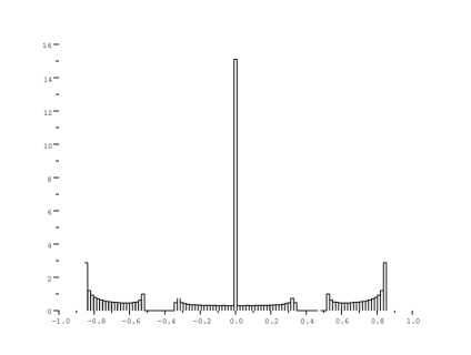
Figure 3: Empirical spectrum

To compute $\left(\mathcal{K}_{n}(f_{\theta})\right)^{-1}$, we use the power series representation of $f_{\theta}$, and truncate this expression after the $15$ first coefficient. This choice ensures that the simulation errors are neglectible with respect to the theoretical ones.

Figure 4 gives the empirical distribution of

$$\sqrt{m_{n}}\sqrt{\int_{\operatorname{Sp}(A)}\left(\frac{f^{\prime}_{\theta}}{f_{\theta}}\right)^{2}}\left(\tilde{\theta}_{n}-\theta_{0}\right).$$

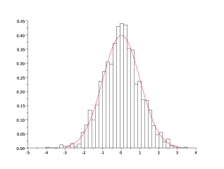
Figure 4: Empirical distribution

6 Appendix

6.1 Szegö’s Lemmas

Szegö’s Lemmas [12] are useful in time series analysis. Indeed, they provide good approximations for the likelihood. As explained in Section 3, these approximations of the likelihood are easier to compute.

In this section, we generalize a weak version of the Szegö Lemmas, for a general graph, under Assumption 3.1 (non expansion criterion for $G_{n}$), and Assumption 3.3 (existence of the spectral measure $\mu$).

For any matrix $(B_{ij})_{i,j\in G_{n}}$, we define the block norm

$$b_{N}(B)=\frac{1}{\delta_{N}}\sum_{i,j\in G_{N}}\left|B_{ij}\right|.$$

We can state the equivalent version of the first Szegö lemma for time-series

Lemma 6.1.

Asymptotic homomorphism

Let $k,n$ be positive integers, and let $g_{1},\cdots,g_{k}$ be analytic functions over $\left[-1,1\right]$ having finite regularity factors (i.e. $\alpha(g_{i})<+\infty,i=1,\cdots,k$). Then,

$$b_{n}\left(\mathcal{K}_{n}(g_{1})\cdots\mathcal{K}_{n}(g_{k})-\mathcal{K}_{n}(g_{1}\cdots g_{k})\right)\leq\frac{k-1}{2}\alpha(g_{1})\cdots\alpha(g_{k}).$$

Corollary 6.1.

For any $g\in\mathcal{F}_{\rho}$ (see the first page of Subsection 3.1 for the definition), and under Assumptions 3.1 and 3.3,

$$\frac{1}{m_{n}}\log\det(\mathcal{K}_{n}(g))\underset{n\rightarrow\infty}{\rightarrow}\int\log(g)\mathrm{d}\mu.$$

Proof.

of Lemma 6.1 This proof follows again the one of [2]. We will prove the result by induction on $k$.

First we deal with the case $k=2$. Let $f$ and $g$ analytic functions over $\left[-1,1\right]$ such that $\alpha(f)<+\infty$ and $\alpha(g)<+\infty$. We write

$$b_{n}(\mathcal{K}_{n}(f)\mathcal{K}_{n}(g)-\mathcal{K}_{n}(fg))$$

$$= \frac{1}{\delta_{n}}\sum_{i,j\in G_{n}}\left|\sum_{k\in G_{n}}\left(\mathcal{K}_{n}(f)\right)_{ik}\left(\mathcal{K}_{n}(g)\right)_{kj}-\sum_{k\in G}\left(\mathcal{K}_{n}(f)\right)_{ik}\left(\mathcal{K}_{n}(g)\right)_{kj}\right|$$

$$= \frac{1}{\delta_{n}}\sum_{i,j\in G_{n}}\sum_{k\in G\backslash G_{n}}\left|\mathcal{K}(f)_{ik}\right|\left|\mathcal{K}(g)_{kj}\right|.$$

Using $\mathcal{K}(g)=\sum_{h=0}^{\infty}g_{h}W^{h}$, Fubini’s theorem gives, since all the previous sequences are in $l^{1}(G)$,

$$b_{n}(\mathcal{K}_{n}(f)\mathcal{K}_{n}(g)-\mathcal{K}_{n}(fg))$$

$$\leq \frac{1}{\delta_{n}}\sum_{i,j\in G_{n}}\sum_{k\in G\backslash G_{n}}\left|\left(\mathcal{K}_{n}(f)\right)_{ik}\left(\mathcal{K}_{n}(g)\right)_{kj}\right|$$

$$\leq \left(\sup_{k\in G\backslash G_{n}}\sum_{i\in G_{n}}\left|\mathcal{K}(f)_{ik}\right|\right)\times\frac{1}{\delta_{n}}\sum_{k\in G\backslash G_{n}}\sum_{j\in G_{n}}\sum_{h=0}^{\infty}\left|g_{h}\right|\left|(W^{h})_{kj}\right|$$

$$\leq \left(\sup_{k\in G}\sum_{i\in G}\left|\mathcal{K}(f)_{ik}\right|\right)\times\sum_{h=0}^{\infty}\left|g_{h}\right|\frac{1}{\delta_{n}}\sum_{k\in G\backslash G_{n}}\sum_{j\in G_{n}}\left|(W^{h})_{kj}\right|.$$

Introducing

$$\Delta_{h}=\sup_{N\in\mathbb{N}}\frac{1}{\delta_{N}}\sum_{k\in G\backslash G_{N}}\sum_{j\in G_{N}}\left|\left(W^{h}\right)_{kj}\right|,$$

we get

$$b_{n}(\mathcal{K}_{n}(f)\mathcal{K}_{n}(g)-\mathcal{K}_{n}(fg))\leq\sup_{k\in G}\sum_{i\in G}\left|\mathcal{K}(f)_{ik}\right|\sum_{h=0}^{\infty}\left|g_{h}\right|\Delta_{h}.$$

The coefficient $\Delta_{h}$ is a porosity factor. It measures the weight of the paths of length $h$ going from the interior of $G_{n}$ to outside.

Note that $\Delta_{h}\leq h+1$, so we get

$$\sum_{h=0}^{\infty}\left|g_{h}\right|\Delta_{h}\leq\alpha(g).$$

Now, we define another norm on $B_{G}$ :

$$\left\|B\right\|_{\infty,in}:=\sup_{k\in G}\sum_{i\in G}\left|B_{ik}\right|,\left(B\in B_{G}\right).$$

We thus obtain

$$\left\|\mathcal{K}(f)\right\|_{\infty,in} = \sup_{k\in G}\sum_{i\in G}\left|\mathcal{K}(f)_{ik}\right|$$

$$\leq \sum_{h=0}^{\infty}\left|f_{h}\right|\left\|W^{h}\right\|_{\infty,in}$$

$$\leq \sum_{h=0}^{\infty}\left|f_{h}\right|\left\|W\right\|_{\infty,in}^{h}$$

$$\leq \sum_{h=0}^{\infty}\left|f_{h}\right|:=\left\|f\right\|_{1,pol}.$$

Finally, we get

$$b_{n}(\mathcal{K}_{G_{n}}(f)\mathcal{K}_{G_{n}}(g)-\mathcal{K}_{G_{n}}(fg))\leq\left\|f\right\|_{1,pol}\alpha(g).$$

To conclude the proof of the lemma, by symmetrization of the last inequality, and since $1\leq(h+1)$, we have,

$$b_{n}\left(\mathcal{K}_{n}(f)\mathcal{K}_{n}(g)-\mathcal{K}_{n}(fg)\right)\leq\frac{1}{2}\alpha(f)\alpha(g).$$ (6)

To perform the inductive step, we need the following inequalities [21]:

$$\alpha(fg) \leq \alpha(f)\alpha(g),$$

$$b_{n}(BC) \leq \left\|B\right\|_{\infty,in}b_{n}(C),$$

$$b_{n}(B+C) \leq b_{n}(B)+b_{n}(C),$$

$$\left\|\mathcal{K}_{n}(f)\right\|_{\infty,in} = \left\|f\right\|_{1,pol}\leq\alpha(f).$$

Let $k>1$, and assume that for all $j\leq k-1$, Lemma 6.1 holds. Under the previous assumptions, and the inductive hypothesis for $k-1$ we get,

$$b_{n}\left(\mathcal{K}_{n}(g_{1})\times\right. \cdots \times\mathcal{K}_{n}(g_{k})-\left.\mathcal{K}_{n}(g_{1}\cdots g_{k})\right)$$

$$\leq \left\|\mathcal{K}_{n}(g_{1})\right\|_{\infty,in}b_{n}\left(\mathcal{K}_{n}(g_{2})\cdots\mathcal{K}_{n}(g_{k})-\mathcal{K}_{n}(g_{2}\cdots g_{k})\right)$$

$$+b_{n}\left(\mathcal{K}_{n}(g_{1})\mathcal{K}_{n}(g_{2}\cdots g_{k})-\mathcal{K}_{n}(g_{1}\cdots g_{k})\right)$$

$$\leq \alpha(g_{1})\frac{k-2}{2}\alpha(g_{2})\cdots\alpha(g_{k})+\frac{1}{2}\alpha(g_{1})\alpha(g_{2}\cdots g_{k})$$

$$\leq \frac{k-1}{2}\alpha(g_{1})\cdots\alpha(g_{k}),$$

which completes the induction step and proves the result. ∎

Proof.

of Corollary 6.1

Let $g\in\mathcal{F}_{\rho}$, and $k$ be a positive integer. Using Lemma 6.1, we have

$$\operatorname{Tr}\left(\mathcal{K}_{n}(g)^{k}-\mathcal{K}_{n}(g^{k})\right)\leq\frac{\delta_{n}}{m_{n}}b_{n}\left(\mathcal{K}_{n}(g)^{k}-\mathcal{K}_{n}(g^{k})\right).$$ (7)

Thus, we have, thanks to Assumption 3.1

$$\frac{1}{m_{n}}\operatorname{Tr}\left(\mathcal{K}_{n}(g)^{k}-\mathcal{K}_{n}(g^{k})\right)\underset{n\rightarrow+\infty}{\rightarrow}0.$$

Denote $\mu_{g}^{[1]}$ the real measure whose $k^{\text{th}}$-moment is given by

$$\int x^{k}\mathrm{d}\mu_{g}^{[1]}=\lim_{n}\frac{1}{m_{n}}\operatorname{Tr}\left(\mathcal{K}_{n}(g)^{k}\right),$$

and $\mu_{g}^{[2]}$ the real measure whose $k^{\text{th}}$-moment is given by

$$\int x^{k}\mathrm{d}\mu_{g}^{[2]}=\lim_{n}\frac{1}{m_{n}}\operatorname{Tr}\left(\mathcal{K}_{n}(g^{k})\right).$$

Notice that both of these measures have support between $\inf g\geq e^{-\rho}>0$ and $\sup g\leq e^{\rho}<+\infty$, since $\alpha(\log(g))<\rho$ (see Section 3). Therefore, the equality of the moments given by Equation 7 gives the equality of the measures $\mu_{g}^{[1]}$ and $\mu_{g}^{[2]}$.

So that, we get

$$\frac{1}{m_{n}}\log\left(\operatorname{det}\left(\mathcal{K}_{n}(g)\right)\right)-\frac{1}{m_{n}}\operatorname{Tr}\left(\mathcal{K}_{n}\left(\log(g)\right)\right)\underset{n\rightarrow+\infty}{\rightarrow}0.$$ (8)

Assumption 3.3 completes the proof of the Corollary since it implies that

$$\frac{1}{m_{n}}\operatorname{Tr}\left(\mathcal{K}_{n}\left(\log(g)\right)\right)\underset{n\rightarrow+\infty}{\rightarrow}\int\log(g)\mathrm{d}\mu.$$

∎

The following lemma enables to replace $\mathcal{K}_{n}(g)$ by the unbiased version $\mathcal{Q}_{n}(g)$ (see Section 3 for the definition).

Lemma 6.2.

Under Assumptions 3.1,3.3, 3.4 and 3.5, and if $f$ or $g$ is a polynomial having degree less than or equal to $P$, we have

$$\left|\frac{1}{m_{n}}\operatorname{Tr}\left(\left(\mathcal{K}_{n}(f)\mathcal{K}_{n}(g)\right)^{p}-\left(\mathcal{K}_{n}(f)\mathcal{Q}_{n}(g)\right)^{p}\right)\right|\leq 2^{p}u_{n}\alpha(f)^{p}\alpha(g)^{p}.$$

Proof.

We define, for any $f$,

$$f_{abs}(x)=\sum_{k}\left|f_{k}\right|x^{k}.$$

Actually, the proof is based of the following idea: as soon as $f$ or $g$ is a polynomial having degree less than or equal to $P$, we have to control only the number of paths of length less than or equal to $P$ (counted with their weights).

Let $p$ be a positive number. Recall that $\mathcal{Q}_{n}(\frac{1}{g})=B^{(n)}\odot\mathcal{K}_{n}(\frac{1}{g})$ (see Section 3), we have,

$$\frac{1}{m_{n}} \left|\operatorname{Tr}\left(\left(\mathcal{K}_{n}(f)\mathcal{K}_{n}(\frac{1}{g})\right)^{p}-\left(\mathcal{K}_{n}(f)\mathcal{Q}_{n}(\frac{1}{g})\right)^{p}\right)\right|$$

$$\leq \frac{1}{m_{n}}\left|\sum_{i\in G_{n}}\sum_{i_{0}=i,i_{1},\cdots,i_{2p}=i}\prod_{l=0\cdots p}B^{(n)}_{i_{2l}i_{2l+1}}\mathcal{K}_{n}(\frac{1}{g})_{i_{2l}i_{2l+1}}\mathcal{K}_{n}(f)_{i_{2l+1}i_{2l+2}}\right.$$

$$-\left.\frac{1}{m_{n}}\sum_{i\in G_{n}}\sum_{i_{0}=i,i_{1},\cdots,i_{2p}=i}\prod_{l=0\cdots p}\mathcal{K}_{n}(\frac{1}{g})_{i_{2l}i_{2l+1}}\mathcal{K}_{n}(f)_{i_{2l+1}i_{2l+2}}\right|$$

$$\leq \frac{1}{m_{n}}\sup_{i_{1},i_{2},\cdots,i_{2p+1}}\left|\prod_{l=0\cdots p-1}B^{(n)}_{i_{2l+1}i_{2l+2}}-1\right|$$

$$\times\sum_{i\in G_{n}}\sum_{i_{0}=i,i_{1},\cdots,i_{2p}=i}\prod_{l=0\cdots p}\left|\mathcal{K}_{n}(\frac{1}{g})_{i_{2l}i_{2l+1}}\mathcal{K}_{n}(f)_{i_{2l+1}i_{2l+2}}\right|$$

$$\leq \frac{1}{m_{n}}\sup_{i_{1},i_{2},\cdots,i_{2p+1}}\left|\prod_{l=0\cdots p-1}B^{(n)}_{i_{2l+1}i_{2l+2}}-1\right|$$

$$\times\sum_{i\in G_{n}}\sum_{i_{0}=i,i_{1},\cdots,i_{2p}=i}\prod_{l=0\cdots p}\mathcal{K}_{n}((\frac{1}{g})_{abs})_{i_{2l}i_{2l+1}}\mathcal{K}_{n}(f_{abs})_{i_{2l+1}i_{2l+2}}$$

$$\leq \sup_{i_{1},i_{2},\cdots,i_{2p+1}}\left|\prod_{l=0\cdots p-1}B^{(n)}_{i_{2l+1}i_{2l+2}}-1\right|\left\|\left(K_{G_{n}}(f_{abs})K_{G_{n}}((\frac{1}{g})_{abs})\right)^{p}\right\|_{2,in}$$

$$\leq \sup_{i_{1},i_{2},\cdots,i_{2p+1}}\left|\prod_{l=0\cdots p-1}B^{(n)}_{i_{2l+1}i_{2l+2}}-1\right|\alpha(f)^{p}\alpha(\frac{1}{g})^{p}.$$

Using Assumption 3.5, we get,

$$\frac{1}{m_{n}} \left|\operatorname{Tr}\left(\left(\mathcal{K}_{n}(f)\mathcal{K}_{n}(\frac{1}{g})\right)^{p}-\left(\mathcal{K}_{n}(f)\mathcal{Q}_{n}(\frac{1}{g})\right)^{p}\right)\right|$$

$$\leq \left|(1+u_{n})^{p}-1\right|\alpha(f)^{p}\alpha(\frac{1}{g})^{p}$$

$$\leq \left|\left(1+u_{n}-1\right)\left((1+u_{n})^{p-1}+(1+u_{n})^{p-2}+\cdots+1\right)\right|\alpha(f)^{p}\alpha(\frac{1}{g})^{p}$$

$$\leq \left|u_{n}\left(2^{p}-1\right)\right|\alpha(f)^{p}\alpha(\frac{1}{g})^{p}$$

$$\leq u_{n}2^{p}\alpha(f)^{p}\alpha(\frac{1}{g})^{p}.$$

This ends the proof of the Lemma. ∎

Finally, the following lemma explains the choice of $B^{(n)}$. The unbiased quadratic form $\mathcal{Q}_{n}$ is no more than a correction of the error between $\mathcal{K}_{n}(f)\mathcal{K}_{n}(g)$ and $\mathcal{K}_{n}(fg)$.

Lemma 6.3 (Exact correction).

Let $f,g\in\mathcal{F}_{\rho}$, and assume that either $f$ or $g$ is a polynomial of degree less than or equal to $P$ (see Section 3). Then, the unbiased quadratic form $\mathcal{Q}_{n}(f_{\theta})$ verify

$$\operatorname{Tr}\left(\mathcal{K}_{n}(f)\mathcal{Q}_{n}(g)\right)=\operatorname{Tr}\left(\mathcal{K}_{n}(fg)\right).$$

Proof.

of Lemma 6.3

First, notice that

$$\operatorname{Tr}\left(\mathcal{K}_{n}(f)\mathcal{Q}_{n}(g)\right)=\sum_{i,j\in G_{n}}\mathcal{K}_{n}(f)_{ij}\mathcal{K}_{n}(g)_{ij}B^{(n)}_{ij}.$$

Since this expression is symmetric on $f,g$, we can now consider the case where $f$ is a polynomial of degree less than or equal to $P$.

Actually, since $f$ is a polynomial, $\mathcal{K}_{n}(f)_{ij}=0$ as soon as $d(i,j)>P$ ($i,j\in G$). Then, if $i,j,k,l\in G$ are such that $\mu_{ij}=\mu_{kl}$, we have

$$\mathcal{K}_{n}(f)_{ij}\mathcal{K}_{n}(g)_{ij}=\mathcal{K}_{n}(f)_{kl}\mathcal{K}_{n}(g)_{kl}.$$

So that, we may here denote, for convenience, $K(f)_{\mu_{ij}}$.

Using Assumption 3.4, this leads to

$$\operatorname{Tr}\left(\mathcal{K}_{n}(f)\mathcal{Q}_{n}(g)\right) = \sum_{i,j\in G_{n}}\mathcal{K}_{n}(f)_{ij}\mathcal{K}_{n}(g)_{ij}B^{(n)}_{ij}$$

$$= \sum_{v\in V_{P}}\sum_{i,j\in G_{n}\atop\mu_{ij}=v,d_{\mathbf{G}}(i,j)\leq P}\mathcal{K}_{n}(f)_{v}\mathcal{K}_{n}(g)_{v}B^{(n)}_{v}$$

$$= \sum_{v\in V_{P}}\mathcal{K}_{n}(f)_{v}\mathcal{K}_{n}(g)_{v}\text{Card}\left\{(i,j)\in G_{n}\times G_{n},\mu_{ij}=v\right\}$$

$$\times\frac{\text{Card}\left\{(i,j)\in G_{n}\times G,\mu_{ij}=v\right\}}{\text{Card}\left\{(i,j)\in G_{n}\times G_{n},\mu_{ij}=v\right\}},$$

$$= \sum_{v\in V_{P}}\sum_{(i,j)\in G_{n}\times G,\atop\mu_{ij}=v,d_{\mathbf{G}}(i,j)\leq P}\mathcal{K}_{n}(f)_{v}\mathcal{K}_{n}(g)_{v}B^{(n)}_{v}$$

$$= \sum_{(i,j)\in G_{n}\times G}\mathcal{K}_{n}(f)_{ij}\mathcal{K}_{n}(g)_{ij}B^{(n)}_{ij}$$

$$= \operatorname{Tr}\left(\mathcal{K}_{n}(fg)\right).$$

That ends the proof of Lemma 6.3. ∎

6.2 Proofs of the lemmas of Theorem 3.1

Recall that the theorem relies on two lemmas. Lemma 3.2 states a condition on deterministic sequences to provide the convergence of the maximizer of these sequences.

Proof.

of Lemma 3.2 Recall that $f_{\theta_{0}}$ denotes the true spectral density. Let $(\ell_{n})_{n\in\mathbb{N}}$ be a deterministic sequence of continuous functions such that

$$\forall\theta\in\Theta,\ell_{n}(\theta_{0})-\ell_{n}(\theta)\underset{n\rightarrow\infty}{\rightarrow}\frac{1}{2}\int\left(-\log(\frac{f_{\theta_{0}}}{f_{\theta}})-1+\frac{f_{\theta_{0}}}{f_{\theta}}\right)\mathrm{d}\mu.$$ (9)

uniformly as $n$ tends to infinity. Denotes moreover $\theta_{n}=\arg\max_{\theta}\ell_{n}(\theta)$. We aim at proving that

$$\theta_{n}\underset{n\rightarrow\infty}{\rightarrow}\theta_{0}.$$

Using the compactness of $\Theta$, let $\theta_{\infty}$ be an accumulation point of the sequence $(\theta_{n})_{n\in\mathbb{N}}$, and $(\theta_{n_{k}})_{k\in\mathbb{N}}$ be a subsequence converging to $\theta_{\infty}$. As the function

$$\theta\mapsto\frac{1}{2}\int\left(-\log(\frac{f_{\theta_{0}}}{f_{\theta}})-1+\frac{f_{\theta_{0}}}{f_{\theta}}\right)\mathrm{d}\mu$$

is continuous on $\Theta$, and the convergence of $(\ell_{n}(\theta_{0})-\ell_{n}(\theta))_{n\in\mathbb{N}}$ is uniform in $\theta$, we have

$$\ell_{n_{k}}(\theta_{0})-\ell_{n_{k}}(\theta_{n_{k}})\xrightarrow{k\rightarrow\infty}\frac{1}{2}\int-\log(\frac{f_{\theta_{0}}}{f_{\theta_{\infty}}})-1+\frac{f_{\theta_{0}}}{f_{\theta_{\infty}}}\mathrm{d}\mu.$$ (10)

But we can notice that, thanks to the definition of $\theta_{n}$, $\ell_{n_{k}}(\theta_{0})-\ell_{n_{k}}(\theta_{n_{k}})\leq 0$ So, since the function $x\mapsto-\log(x)+x-1$ is non negative and vanishes if, and only if, $x=1$, we get that $f_{\theta_{0}}=f_{\theta_{\infty}}$. By injectivity of the function $\theta\rightarrow f_{\theta}$, we get $\theta_{\infty}=\theta_{0}$, for any accumulation point $\theta_{\infty}$ of the sequence $(\theta_{n})_{n\in\mathbb{N}}$, which ends the proof of this first lemma. ∎

Lemma 3.1 provides the uniform convergence of the contrasts of maximum likelihood and approximated maximum likelihood to the Kullback information. The proof may be cut into several lemmas.

Proof.

of Lemma 3.1

First, notice that by construction, we have, for any $\theta\in\Theta$,

$$\mathbb{IK}(f_{\theta_{0}},f_{\theta})=\lim_{n}\mathbb{E}\left[\frac{1}{m_{n}}\left(L_{n}(f_{\theta_{0}},X_{n})-L_{n}(f_{\theta},X_{n})\right)\right],$$ (11)

when it exists. Then, we can compute

$$l_{n}(f_{\theta_{0}},X_{n})-l_{n}(f_{\theta},X_{n}) = -\frac{1}{2m_{n}}\left(\log\det(\mathcal{K}_{n}(f_{\theta_{0}}))-\log\det(\mathcal{K}_{n}(f_{\theta}))\right)$$

$$-\frac{1}{2m_{n}}\left(X_{n}^{T}\mathcal{K}_{n}(f_{\theta_{0}})^{-1}X_{n}-X_{n}^{T}\mathcal{K}_{n}(f_{\theta})^{-1}X_{n}\right)$$

Corollary 6.1 of Lemma 6.1 provides the following convergence

$$\frac{1}{m_{n}}\left(\log\det(\mathcal{K}_{n}(f_{\theta_{0}}))-\log\det(\mathcal{K}_{n}(f_{\theta}))\right)\underset{n\rightarrow\infty}{\rightarrow}\int\log\left(\frac{f_{\theta_{0}}}{f_{\theta}}\right)\mathrm{d}\mu.$$ (12)

To prove the existence of $\mathbb{IK}(f_{\theta_{0}},f_{\theta})$, it only remains to prove the $\mathbb{P}_{f_{\theta_{0}}}$-a.s. convergence of $\frac{1}{m_{n}}X_{n}^{T}\mathcal{K}_{n}(f_{\theta})^{-1}X_{n}$ to $\int\frac{f_{\theta_{0}}}{f_{\theta}}\mathrm{d}\mu$ as $n$ goes to infinity.

This is ensured by the following Lemma.

Lemma 6.4 (Convergence lemma).

For respectively $\Lambda=\mathcal{K}_{n}(\frac{1}{f_{\theta}})$, $\Lambda=(\mathcal{K}_{n}(f_{\theta}))^{-1}$ or $\Lambda=\mathcal{Q}_{n}(\frac{1}{f_{\theta}})$, we have,

$$\frac{1}{m_{n}}X_{n}^{T}\Lambda X_{n}\underset{n\rightarrow\infty}{\rightarrow}\int\frac{f_{\theta_{0}}}{f_{\theta}}\mathrm{d}\mu,\mathbb{P}_{f_{\theta_{0}}}-\text{a.s.}.$$

Lemma 6.4 combined with Corollary 6.1 ensures the $\mathbb{P}_{f_{\theta_{0}}}-\text{a.s.}$ convergence of $\tilde{l}_{n}(f_{\theta_{0}})-\tilde{l}_{n}(f_{\theta})$, $\bar{l}_{n}(f_{\theta_{0}})-\bar{l}_{n}(f_{\theta})$ to $\mathbb{IK}(f_{\theta_{0}},f_{\theta})$. It provides also the $\mathbb{P}_{f_{\theta_{0}}}-\text{a.s.}$ convergence of $l^{(u)}_{n}(f_{\theta_{0}})-l^{(u)}_{n}(f_{\theta})$ to $\mathbb{IK}(f_{\theta_{0}},f_{\theta})$ in the $AR_{P}$ or $MA_{P}$ cases (see Section 3). To complete the assertion of Lemma 3.1, it only remains to show the uniform convergences on $\Theta$ of the last quantities. This will be done using an equicontinuity argument given by the following Lemma.

Lemma 6.5 (Equicontinuity lemma).

For all $n\geq 0$, the sequences of functions

$$\left(l_{n}(f_{\theta_{0}},X_{n})-l_{n}(f_{\theta},X_{n})\right)_{n\in\mathbb{N}}$$

is an $\mathbb{P}_{f_{\theta_{0}}}$-a.s. equicontinuous sequence on $\left(\left\{f_{\theta},\theta\in\Theta\right\},\left\|.\right\|_{\infty}\right)$.This property also holds for $\bar{l_{n}}$,$\tilde{l}_{n}$. Furthermore, the sequence $\left(l^{(u)}_{n}(f_{\theta_{0}},X_{n}-l_{n}^{(u)}(f_{\theta},X_{n})\right)_{n\in\mathbb{N}}$ is also $\mathbb{P}_{f_{\theta_{0}}}$-a.s. equicontinuous, on $\left(\left\{f_{\theta},\theta\in\Theta\right\},\left\|.\right\|_{1,pol}\right)$.

We can now end the proof of Lemma 3.1:

First, notice that the space $\left\{f_{\theta},\theta\in\Theta\right\}$ is compact for the topology of the uniform convergence. This also holds for $\left(\left\{f_{\theta},\theta\in\Theta\right\},\left\|.\right\|_{1,pol}\right)$. So, there exists a dense sequence $(f_{\theta_{p}})_{p\in\mathbb{N}}$. Then, using Lemma 6.1 and Corollary 6.1, the sequence $\left(l_{n}(f_{\theta_{0}},X_{n})-l_{n}(f_{\theta_{p}},X_{n})\right)_{n\in\mathbb{N}}$ converges $\mathbb{P}_{f_{\theta_{0}}}$-a.s. to $\mathbb{IK}(f_{\theta_{0}},f_{\theta_{p}})$.

If a sequence of functions is equicontinuous and converges pointwise on a dense subset of its domain, and if its co-domain is a complete space, then the sequence converges pointwise on all the domain [20].

Using this well known property, we obtain, $\mathbb{P}_{f_{\theta_{0}}}$-a.s., the pointwise convergence of

$$\left(l_{n}(f_{\theta_{0}},X_{n})-l_{n}(f_{\theta},X_{n})\right)_{n\in\mathbb{N}}$$

to $\mathbb{IK}(f_{\theta_{0}},f_{\theta})$, for any $\theta\in\Theta$.

Furthermore, if a sequence of functions is equicontinuous and converges pointwise on its domain, then this convergence is uniform on any compact subspace of the domain [20].

Thus, we get, $\mathbb{P}_{f_{\theta_{0}}}$-a.s., the uniform convergence on $\Theta$ of the sequence

$$\left(l_{n}(f_{\theta_{0}},X_{n})-l_{n}(f_{\theta},X_{n})\right)_{n\in\mathbb{N}}$$

to $\mathbb{IK}(f_{\theta_{0}},f_{\theta})$.

Using the same kind of arguments, this uniform convergence also holds for $\bar{l_{n}}$,$\tilde{l}_{n}$ and $l^{(u)}_{n}$. This concludes the proof of Lemma 3.1.

∎

6.3 Proof of the technical lemmas

Proof.

of Lemma 6.4

Let $\theta\in\Theta$. First, consider the case $\Lambda_{n}=\mathcal{K}_{n}\left(\frac{1}{f_{\theta}}\right)$. We aim at proving that

$$\frac{1}{m_{n}}X_{n}^{T}\Lambda_{n}X_{n}\underset{n\rightarrow\infty}{\rightarrow}\int\frac{f_{\theta_{0}}}{f_{\theta}}\mathrm{d}\mu,\mathbb{P}_{f_{\theta_{0}}}-\text{a.s.}.$$

To do that, we make use of classical tools of large deviation (see [9]). We compute the Laplace transform of $X_{n}^{T}\Lambda_{n}X_{n}$ :

$$\mathbb{E}_{\mathbb{P}_{f_{\theta_{0}}}} \left[e^{\lambda X_{n}^{T}\mathcal{K}_{n}(\frac{1}{f_{\theta}})X_{n}}\right]$$

$$= \frac{1}{(\sqrt{2\pi})^{m_{n}}\sqrt{\det(\mathcal{K}_{n}({f_{\theta_{0}}))}}}\int e^{\frac{1}{2}X_{n}^{T}\left(\left(\mathcal{K}_{n}(f_{\theta_{0}})\right)^{-1}-2\lambda\mathcal{K}_{n}(\frac{1}{f_{\theta}})\right)X_{n}}$$

$$= \frac{1}{\sqrt{\det(\mathcal{K}_{n}(f_{\theta_{0}})})}\sqrt{\det\left(\left[\left(\mathcal{K}_{n}(f_{\theta_{0}})\right)^{-1}-2\lambda\mathcal{K}_{n}(\frac{1}{f_{\theta}})\right]^{-1}\right)}$$

$$= \frac{1}{\sqrt{\det\left(I_{G_{n}}-2\lambda\mathcal{K}_{n}(f_{\theta_{0}})^{\frac{1}{2}}\mathcal{K}_{n}(\frac{1}{f_{\theta}})\mathcal{K}_{n}(f_{\theta_{0}})^{\frac{1}{2}}\right)}}.$$

These last equalities hold as soon as $I_{G_{n}}-2\lambda\mathcal{K}_{n}(f_{\theta_{0}})^{\frac{1}{2}}\mathcal{K}_{n}(\frac{1}{f_{\theta}})\mathcal{K}_{n}(f_{\theta_{0}})^{\frac{1}{2}}$ is positive. This is true whenever $\lambda\leq 0$ or small enough.

Now, for $\lambda\leq 0$, define

$$\phi_{n}(\lambda):=\frac{1}{m_{n}}\log\left(\right.\mathbb{E}_{\mathbb{P}_{f_{\theta_{0}}}}\left.\left[e^{\lambda X_{n}^{T}\mathcal{K}_{n}(\frac{1}{f_{\theta}})X_{n}}\right]\right),$$

This function verifies

$$\phi_{n}(\lambda)=-\frac{1}{2m_{n}}\log\det\left(I_{G_{n}}-2\lambda\mathcal{K}_{n}(f_{\theta_{0}})^{\frac{1}{2}}\mathcal{K}_{n}(\frac{1}{f_{\theta}})\mathcal{K}_{n}(f_{\theta_{0}})^{\frac{1}{2}}\right).$$

Define also

$$\phi(\lambda)=\lim_{n}\phi_{n}(\lambda),$$

We get, using Corollary 6.1,

$$\phi(\lambda)=-\frac{1}{2}\int\log\left(1-2\lambda\frac{f_{\theta_{0}}}{f_{\theta}}\right).$$

We can also compute

$$\phi^{\prime\prime}(\lambda)=\int\frac{2(\frac{f_{\theta_{0}}}{f_{\theta}})^{2}}{(1-2\lambda\frac{f_{\theta_{0}}}{f_{\theta}})^{2}}\mathrm{d}\mu>0.$$

As very usual, we define the convex conjugate of $\phi$ by

$$\phi^{*}(t):=\sup_{\lambda\in\mathbb{R}^{-}}\left[\lambda t-\phi(\lambda)\right],t\in\mathbb{R}.$$

As soon as $\phi$ is strictly convex, $\phi^{*}(t)>\phi(0)=0$, for any $t\neq\phi^{\prime}(0)=\int\frac{f}{g}\mathrm{d}\mu$.

We can now write, for $\lambda\leq 0$,

$$\frac{1}{m_{n}}\log(\mathbb{P}(\frac{1}{m_{n}}X_{n}^{T}\Lambda_{n}X_{n}\geq t)) =\frac{1}{m_{n}}\log(\mathbb{P}(e^{\lambda X_{n}^{T}\Lambda_{n}X_{n}}\geq e^{m_{n}\lambda t}))$$

$$\leq\frac{1}{m_{n}}\log\left(e^{-m_{n}\lambda t}\right)+\frac{1}{m_{n}}\log\left(\mathbb{E}[e^{\lambda X_{n}^{T}\Lambda_{n}X_{n}}]\right)$$

$$\leq-\lambda t+\phi_{n}(\lambda).$$

Then we get, $\forall t>\int\frac{f}{g}\mathrm{d}\mu$,

$$\limsup_{n}\left(\frac{1}{m_{n}}\log(\mathbb{P}(\frac{1}{m_{n}}X_{n}^{T}\Lambda_{n}X_{n}\geq t))\right)\leq-\lambda t+\phi(\lambda)$$

So that, taking the infimum on $\lambda$, we get

$$\limsup_{n}\left(\frac{1}{m_{n}}\log(\mathbb{P}(\frac{1}{m_{n}}X_{n}^{T}\Lambda_{n}X_{n}\geq t))\right)\leq-\phi^{*}(t)<0$$

We can obtain the same bound for $t<\int\frac{f}{g}\mathrm{d}\mu$. By Borel-Cantelli theorem, we get the $\mathbb{P}_{f_{\theta_{0}}}$-almost sure convergence of $\frac{1}{m_{n}}X_{n}^{T}\Lambda_{n}X_{n}$ to $\int\frac{f}{g}\mathrm{d}\mu$. To prove the same convergence with $\Lambda_{n}=(\mathcal{K}_{n}(f_{\theta}))^{-1}$, we have to show that the difference between the spectral empirical measure of $\mathcal{K}_{n}(f_{\theta_{0}})^{\frac{1}{2}}\mathcal{K}_{n}(\frac{1}{f_{\theta}})\mathcal{K}_{n}(f_{\theta_{0}})^{\frac{1}{2}}$ and $\mathcal{K}_{n}(f_{\theta_{0}})^{\frac{1}{2}}\mathcal{K}_{n}(f_{\theta})^{-1}\mathcal{K}_{n}(f_{\theta_{0}})^{\frac{1}{2}}$ converges weakly to zero. It is sufficient to control the convergence of every moment, because these two last measures both have compact support.

For this, we make use of the Schatten norms. For any $A,B$ matrices of $M_{m_{n}}(\mathbb{R})$, we define

$$\left\|A\right\|_{Sch,p}=\left(\sum s_{k}(A)^{p}\right)^{\frac{1}{p}},$$

where $s_{k}(A)$ are the singular values of $A$.

Note that

$$\left|Tr(AB)\right|\leq\left\|AB\right\|_{Sch,1}\leq\left\|A\right\|_{Sch,1}\left\|B\right\|_{Sch,\infty}.$$

Recall that since $f_{\theta}\in\mathcal{F}_{\rho}$, we have $e^{-\rho}\leq f_{\theta}\leq e^{\rho}$. Hence, for any $p\geq 1$,

$$\frac{1}{m_{n}}\left|\operatorname{Tr}\Bigl{(}\mathcal{K}_{n}^{p}{(\frac{1}{f_{\theta}})}\right. \mathcal{K}_{n}^{p}(f_{\theta_{0}})-\left.\mathcal{K}_{n}^{-p}(f_{\theta})\mathcal{K}_{n}^{p}(f_{\theta_{0}})\Bigl{)}\right|$$

$$\leq\frac{1}{m_{n}}\left\|\mathcal{K}_{n}{(f_{\theta})}^{-p}\mathcal{K}_{n}^{p}(f_{\theta_{0}})\right\|_{Sch,\infty}\left\|\left(\mathcal{K}_{n}^{p}{(\frac{1}{\theta})}\mathcal{K}_{n}^{p}(f_{\theta})-I_{G_{n}}\right)\right\|_{Sch,1}$$

$$\leq\frac{\delta_{n}}{m_{n}}\frac{e^{2\rho p}}{e^{-2\rho p}}\alpha(f_{\theta})^{2p}\alpha(\frac{1}{f_{\theta}})^{2p}\underset{n\rightarrow\infty}{\rightarrow}0.$$

To obtain the same bound with $\Lambda_{n}=\mathcal{Q}_{n}(\frac{1}{f_{\theta}})$, we have to prove that the difference between the spectral empirical measures of $\mathcal{K}_{n}(f_{\theta_{0}})^{\frac{1}{2}}\mathcal{K}_{n}(\frac{1}{f_{\theta}})\mathcal{K}_{n}(f_{\theta_{0}})^{\frac{1}{2}}$ and $\mathcal{K}_{n}(f_{\theta_{0}})^{\frac{1}{2}}\mathcal{Q}_{n}(\frac{1}{f_{\theta}})\mathcal{K}_{n}(f_{\theta_{0}})^{\frac{1}{2}}$ converge weakly to zero. This last assertion is a direct consequence of Lemma 6.2. So, we get

$$\frac{1}{m_{n}}X_{n}^{T}\Lambda_{n}X_{n}\rightarrow\int\frac{f_{\theta_{0}}}{f_{\theta}},\mathbb{P}_{f_{\theta_{0}}}-\text{ a.s.}$$

∎

Proof.

of Lemma 6.5

Recall that we aim at proving that, $\mathbb{P}_{f_{\theta_{0}}}$-a.s., the sequence of functions

$$\left(l_{n}(f_{\theta_{0}},X_{n})-l_{n}(f_{\theta},X_{n})\right)_{n\in\mathbb{N}}$$

is equicontinuous on $\left\{f_{\theta},\theta\in\Theta\right\}$, and that this property also holds for $\bar{l_{n}}$,$\tilde{l}_{n}$ and $l^{(u)}_{n}$.

First, we will prove the equicontinuity of the sequence

$$\left(\frac{1}{m_{n}}\log\det(\mathcal{K}_{n}(f_{\theta}))\right)_{n\in\mathbb{N}}.$$

Let $\theta,\theta^{\prime}\in\Theta$.

Denote $\lambda_{i}$ the eigenvalues of $\mathcal{K}_{n}(f_{\theta^{\prime}})^{-1}\left(\mathcal{K}_{n}(f_{\theta^{\prime}})-\mathcal{K}_{n}(f_{\theta})\right)$. Since $f_{\theta}\in\mathcal{F}_{\rho}$, we have $e^{-\rho}\leq f_{\theta}\leq e^{\rho}$.

Notice that we have

$$\sup_{i=1,\cdots,n}\left|\lambda_{i}\right| =\left\|\mathcal{K}_{n}(f_{\theta^{\prime}})^{-1}\left(\mathcal{K}_{n}(f_{\theta^{\prime}})-\mathcal{K}_{n}(f_{\theta})\right)\right\|_{2,op}$$

$$\leq e^{\rho}\left\|f_{\theta^{\prime}}-f_{\theta}\right\|_{\infty}.$$

So that, to prove the equicontinuity, we may assume that $\theta$ is close enough to $\theta^{\prime}$ to ensure that $\sup_{i=1,\cdots,n}\left|\lambda_{i}\right|\leq\frac{1}{2}$.

We have

$$\frac{1}{m_{n}}\Big{|}\log\det(\mathcal{K}_{n}(f_{\theta^{\prime}})) -\log\det(\mathcal{K}_{n}(f_{\theta}))\Big{|}$$

$$=\frac{1}{m_{n}}\left|\log\det\left(I_{G_{n}}-\mathcal{K}_{n}(f_{\theta_{0}})^{-1}\left(\mathcal{K}_{n}(f_{\theta^{\prime}})-\mathcal{K}_{n}(f_{\theta})\right)\right)\right|$$

$$\leq\frac{1}{m_{n}}\sum_{i\in G_{n}}\left|\log(1+\lambda_{i})\right|$$

$$\leq\frac{1}{m_{n}}\sup_{i\in G_{n}}\left|\log(1+\lambda_{i})\right|$$

$$\leq 2\log(2)\sup_{i\in G_{n}}\left|\lambda_{i}\right|$$

$$\leq 2\log(2)e^{\rho}\left\|f_{\theta^{\prime}}-f_{\theta}\right\|_{\infty}.$$

Furthermore, the sequence $(\int\log(f_{\theta})\mathrm{d}\mu)_{n\in\mathbb{N}}$ is also equicontinuous since, using a Taylor formula,

$$\int\left|\log(f_{\theta^{\prime}})\mathrm{d}\mu-\int\log(f_{\theta})\mathrm{d}\mu\right|\leq e^{\rho}\left\|f_{\theta^{\prime}}-f_{\theta}\right\|_{\infty}.$$

Now we tackle the equicontinuity of the sequences

$$\left(X_{n}^{T}\mathcal{K}_{n}(f_{\theta})^{-1}X_{n}\right)_{n\in\mathbb{N}},$$

$$\left(X_{n}^{T}\mathcal{K}_{n}(\frac{1}{f_{\theta}})X_{n}\right)_{n\in\mathbb{N}}$$

and

$$\left(X_{n}^{T}\mathcal{Q}_{n}(\frac{1}{f_{\theta}})X_{n}\right)_{n\in\mathbb{N}}.$$

Notice first that, for any matrix $B\in M_{n}(\mathbb{R})$,

$$\frac{1}{m_{n}}\left|X_{n}^{T}BX_{n}\right|\leq\frac{1}{m_{n}}\left\|B\right\|_{2,op}\left|X_{n}^{T}X_{n}\right|.$$

It is thus sufficient to prove the equicontinuity of the sequences

$$(\mathcal{K}_{n}(f_{\theta})^{-1})_{n\in\mathbb{N}},$$

$$(\mathcal{K}_{n}(\frac{1}{f_{\theta}}))_{n\in\mathbb{N}}$$

and

$$(\mathcal{Q}_{n}(f_{\theta})^{-1})_{n\in\mathbb{N}},$$

for the norm $\left\|.\right\|_{2,op}$

Note that

$$\left\|\mathcal{K}_{n}(\frac{1}{f_{\theta^{\prime}}})-\mathcal{K}_{n}(\frac{1}{f_{\theta}})\right\|_{2,op} \leq\left|\frac{1}{f_{\theta^{\prime}}}-\frac{1}{f_{\theta}}\right|_{\infty}$$

$$\leq e^{2\rho}\left\|f_{\theta^{\prime}}-f_{\theta}\right\|_{\infty}.$$

Then,

$$\left\|(\mathcal{K}_{n}(f_{\theta^{\prime}}))^{-1}-(\mathcal{K}_{n}(f_{\theta}))^{-1}\right\|_{2,op} \leq\left\|(\mathcal{K}_{n}(f_{\theta^{\prime}}))^{-1}(\mathcal{K}_{n}(f_{\theta}))^{-1}\right\|_{2,op}\left\|(\mathcal{K}_{n}(f_{\theta^{\prime}}))-(\mathcal{K}_{n}(f_{\theta}))\right\|_{2,op}$$

$$\leq e^{2\rho}\left\|f_{\theta^{\prime}}-f_{\theta}\right\|_{\infty}.$$

Then, recall that, for any symmetric matrix $B\in M_{n}(\mathbb{R})$, we have

$$\left\|B\right\|_{2,op}\leq\left\|B\right\|_{\infty,op}.$$

Recall also that $\mathcal{Q}_{n}(f_{\theta})=B^{(n)}\odot\mathcal{K}_{n}(f_{\theta})$. Denote

$$\left\|\mathcal{Q}_{n}(\frac{1}{f_{\theta^{\prime}}})-\mathcal{Q}_{n}(\frac{1}{f_{\theta}})\right\|_{2,op} \leq \left\|\mathcal{Q}_{n}(\frac{1}{f_{\theta^{\prime}}})-\mathcal{Q}_{n}(\frac{1}{f_{\theta}})\right\|_{\infty,op}$$

$$\leq \sup_{i,j=1,\cdots n}\left|B^{(n)}_{ij}\right|\left\|\mathcal{K}_{n}(\frac{1}{f_{\theta^{\prime}}})-\mathcal{K}_{n}(\frac{1}{f_{\theta}})\right\|_{\infty,op}$$

$$\leq (1+u_{n})\left\|\frac{1}{f_{\theta^{\prime}}}-\frac{1}{f_{\theta}}\right\|_{1,pol}(\text{see Assumption }\ref{hyp_unbiased}).$$

Since the map $f_{\theta}\mapsto\frac{1}{f_{\theta}}$ is continuous over $\mathcal{F}_{\rho}$, which is compact, we get the uniform equicontinuity of the map $f_{\theta}\mapsto X_{n}^{T}\mathcal{Q}_{n}(\frac{1}{f_{\theta}})X_{n}$ (for the norm $\left\|.\right\|_{1,pol}$).

This concludes the proof of Lemma 6.5 ∎

Proof.

of Lemma 3.3

We aim at proving the asymptotic normality of $\sqrt{m_{n}}(l_{n}^{(u)})^{\prime}(\theta_{0})$.

Using the Fourier transform, it is sufficient to prove that

$$\lim_{n}\mathbb{E}\left[\exp\left(i\sqrt{m_{n}}t\left((l_{n}^{(u)})^{\prime}(\theta_{0})\right)\right)\right]=\exp\left(-\int\frac{1}{4}t^{2}\frac{(f^{\prime}_{\theta_{0}})^{2}}{f_{\theta_{0}}^{2}}(t)\mathrm{d}\mu(t)\right)$$

Recall that we have

$$(l_{n}^{(u)})^{\prime}(\theta)=-\frac{1}{2}\int\frac{f^{\prime}_{\theta}}{f_{\theta}}\mathrm{d}\mu+\frac{1}{2m_{n}}X_{n}^{T}\mathcal{Q}_{n}(\frac{f^{\prime}_{\theta}}{f_{\theta}^{2}})X_{n}.$$

We can compute

$$\sqrt{m_{n}}\mathbb{E} \left[(l_{n}^{(u)})^{\prime}(\theta_{0})\right]=\sqrt{m_{n}}\left(-\frac{1}{2}\int\frac{f^{\prime}_{\theta_{0}}}{f_{\theta_{0}}}\mathrm{d}\mu+\frac{1}{2m_{n}}\operatorname{Tr}\left(\mathcal{K}_{n}(f_{\theta_{0}})\mathcal{Q}_{n}(\frac{f^{\prime}_{\theta}}{f_{\theta}^{2}})\right)\right)$$

$$=\sqrt{m_{n}}\left(-\frac{1}{2}\int\frac{f^{\prime}_{\theta_{0}}}{f_{\theta_{0}}}\mathrm{d}\mu+\frac{1}{2m_{n}}\operatorname{Tr}\left(\mathcal{K}_{n}\left(f_{\theta_{0}}\frac{f^{\prime}_{\theta_{0}}}{f_{\theta_{0}}^{2}}\right)\right)\right)(\text{see Lemma }\ref{l:correction})$$

$$\leq Cv_{n}\sqrt{m_{n}}\underset{n\rightarrow\infty}{\rightarrow}0~{}(\text{see Assumption }\ref{hyp_norm}).$$

If we define

$$Z_{n}=t\frac{1}{2m_{n}}X^{T}\mathcal{Q}_{n}(\frac{f^{\prime}_{\theta}}{f_{\theta}^{2}})X,$$

and

$$Z=t\frac{1}{2}\int\frac{f^{\prime}_{\theta}}{f_{\theta}}\mathrm{d}\mu,$$

the last equality means that

$$\sqrt{m_{n}}\left(\mathbb{E}\left[Z_{n}\right]-Z\right)\rightarrow 0.$$

This holds only if $f_{\theta_{0}}$ is a polynomial, or if all the $f_{\theta},\theta\in\Theta$ are polynomials. This brings out that the second theorem holds for the $AR_{P}$ or $MA_{P}$ case. It also explains the term ’unbiased estimator’ used for $\theta^{(u)}$.

Then, it is sufficient to show

$$\lim_{n}\mathbb{E}\left[\exp\left(i\sqrt{m_{n}}\left(Z_{n}-\mathbb{E}\left[Z_{n}\right]\right)\right)\right]=\exp\left(-\int\frac{1}{4}t^{2}\frac{(f^{\prime}_{\theta_{0}})^{2}(t)}{f_{\theta_{0}}^{2}(t)}\mathrm{d}\mu(t)\right).$$

If $\tau_{k}$ denotes the eigenvalues of the symmetric matrix

$$M_{n}:=\frac{t}{2}\mathcal{K}_{n}(f_{\theta_{0}})^{\frac{1}{2}}\mathcal{Q}_{n}(\frac{f^{\prime}_{\theta_{0}}}{f_{\theta_{0}}^{2}})\mathcal{K}_{n}(f_{\theta_{0}})^{\frac{1}{2}},$$

then we can write

$$Z_{n}=\frac{1}{m_{n}}\sum_{k=1}^{m_{n}}\tau_{k}Y_{k}^{2}.$$

where $(Y_{k})_{k\in G_{n}}$ has the standard Gaussian distribution on $\mathbb{R}^{m_{n}}$.

The independence of $Y_{k}$ leads to

$$\log\left(\mathbb{E}\left[\exp\left(i\sqrt{m_{n}}\left(Z_{n}-\mathbb{E}\left[Z_{n}\right]\right)\right)\right]\right)=-\sum_{k=1}^{m_{n}}\left(i\frac{\tau_{k}}{\sqrt{m_{n}}}+\frac{1}{2}\log(1-2i\frac{\tau_{k}}{\sqrt{m_{n}}})\right).$$

The $\tau_{k}$ are bounded, thanks to the following inequality:

$$\left\|M_{n}\right\|_{2,op} = \left\|\frac{t}{2}\mathcal{K}_{n}(f_{\theta_{0}})^{\frac{1}{2}}\mathcal{Q}_{n}(\frac{f^{\prime}_{\theta_{0}}}{f_{\theta_{0}}^{2}})\mathcal{K}_{n}(f_{\theta_{0}})^{\frac{1}{2}}\right\|_{2,op}$$

$$\leq \left\|\frac{t}{2}\mathcal{K}_{n}(f_{\theta_{0}})^{\frac{1}{2}}\right\|_{2,op}\left\|\mathcal{Q}_{n}(\frac{f^{\prime}_{\theta_{0}}}{f_{\theta_{0}}^{2}})\right\|_{2,op}\left\|\mathcal{K}_{n}(f_{\theta_{0}})^{\frac{1}{2}}\right\|_{2,op}$$

$$\leq \left\|\frac{t}{2}\mathcal{K}_{n}(f_{\theta_{0}})^{\frac{1}{2}}\right\|_{2,op}\left\|\mathcal{Q}_{n}(\frac{f^{\prime}_{\theta_{0}}}{f_{\theta_{0}}^{2}})\right\|_{1,op}\left\|\mathcal{K}_{n}(f_{\theta_{0}})^{\frac{1}{2}}\right\|_{2,op}$$

$$\leq e^{\rho}\alpha(f^{\prime}_{\theta_{0}})\alpha(f_{\theta_{0}})^{2}(1+u_{n}).$$

The Taylor expansion of $\log(1-2\frac{\tau_{k}}{\sqrt{m_{n}}})$ gives

$$\log\left(\mathbb{E}\left[\exp\left(i\sqrt{m_{n}}\left(Z_{n}-\mathbb{E}\left[Z_{n}\right]\right)\right)\right]\right)=-\frac{1}{m_{n}}\sum_{k=1}^{m_{n}}\tau_{k}^{2}+R_{n}.$$

With $\left|R_{n}\right|\leq C\frac{1}{m_{n}\sqrt{m_{n}}}\sum_{k=1}^{m_{n}}\left|\tau_{k}\right|^{3}$

Since the $\tau_{k}$ are bounded the assertion will be proved if we show that

$$\frac{1}{m_{n}}\operatorname{Tr}(M_{n}^{2})=\frac{1}{m_{n}}\sum_{k=1}^{m_{n}}\tau_{k}^{2}\xrightarrow{n\rightarrow\infty}\int\frac{1}{4}t^{2}\frac{(f^{\prime}_{\theta_{0}})^{2}(t)}{f_{\theta_{O}}^{2}(t)}\mathrm{d}\mu(t).$$

This last convergence is a consequence of Lemmas 6.1 and 6.2.

This provides the asymptotic normality of $\sqrt{m_{n}}(l_{n}^{(u)})^{\prime}(\theta_{0})$ and concludes the proof of Lemma 3.3:

$$\sqrt{m_{n}}(l_{n}^{(u)})^{\prime}(\theta_{0})\underset{n\rightarrow\infty}{\rightarrow}\mathcal{N}(0,\frac{1}{2}\int\left(\frac{f^{\prime}_{\theta_{0}}}{f_{\theta_{0}}}\right)^{2}\mathrm{d}\mu).$$

∎

Proof.

of Lemma 3.4

We aim now at proving the $P_{f_{\theta_{0}}}$-a.s. following convergence:

$$\left((l_{n}^{(u)})^{\prime\prime}(\breve{\theta}_{n})\right)^{-1}\underset{n\rightarrow\infty}{\rightarrow}\frac{1}{2}\left(\int\frac{(f^{\prime}_{\theta_{0}})^{2}}{f_{\theta_{0}}^{2}}\mathrm{d}\mu\right)^{-1}$$

We have

$$(l_{n}^{(u)})^{\prime\prime}(\theta)=-\frac{1}{2m_{n}}\left(\int\frac{f^{\prime\prime}_{\theta}f_{\theta}-(f^{\prime}_{\theta})^{2}}{f_{\theta}^{2}}\mathrm{d}\mu+X_{n}^{T}\mathcal{Q}_{n}\left(\frac{2(f^{\prime}_{\theta})^{2}-f^{\prime\prime}_{\theta}f_{\theta}}{f^{3}_{\theta}}\right)X_{n}\right),$$

which leads to

$$(l_{n}^{(u)})^{\prime\prime}(\theta)\underset{n\rightarrow\infty}{\rightarrow}\frac{1}{2}\int\left(\frac{f^{\prime\prime}_{\theta}f_{\theta}-(f^{\prime}_{\theta})^{2}}{f_{\theta}^{2}}+\frac{f_{\theta_{0}}\big{(}2(f^{\prime}_{\theta})^{2}-f^{\prime\prime}_{\theta}f_{\theta}\big{)}}{f^{3}_{\theta}}\right)\mathrm{d}\mu,P_{f_{\theta_{0}}}\text{-a.s.}$$

Since the sequence $l_{n}^{(u)}$ is equicontinuous and $\breve{\theta}_{n}\underset{n\rightarrow\infty}{\rightarrow}\theta_{0}$, we obtain the desired convergence :

$$(l_{n}^{(u)})^{\prime\prime}(\breve{\theta}_{n})\underset{n\rightarrow\infty}{\rightarrow}\frac{1}{2}\int\left(\frac{(f^{\prime}_{\theta_{0}})^{2}}{f_{\theta_{0}}^{2}}\right)\mathrm{d}\mu,P_{f_{\theta_{0}}}\text{-a.s.}$$

∎

Proof.

of Lemma 3.5

We want to compute the asymptotic Fisher information. As usual, it is sufficient to compute

$$\frac{1}{m_{n}}\operatorname{Var}\left(L^{\prime}_{n}(\theta_{0})\right)=\lim_{n}\frac{1}{2m_{n}}\operatorname{Tr}(M_{n}(\theta_{0})^{2}),$$

where $M_{n}(\theta)=\mathcal{K}_{n}(f_{\theta})^{-1}\mathcal{K}_{n}(f^{\prime}_{\theta})\mathcal{K}_{n}(f_{\theta})^{-1}\mathcal{K}_{n}(f_{\theta_{0}})$.

This leads, together with Lemma 6.1, and Assumption 3.3 to

$$\frac{1}{m_{n}}\operatorname{Var}\left(L^{\prime}_{n}(\theta_{0})\right)\rightarrow\frac{1}{2}\int\frac{(f^{\prime}_{\theta_{0}})^{2}}{f_{\theta_{0}}^{2}}\mathrm{d}\mu.$$

This ends the proof of the last lemma. ∎

References

- [1] David Aldous and Russell Lyons. Processes on unimodular random networks. Electron. J. Probab., 12:no. 54, 1454–1508, 2007.
- [2] R. Azencott and D. Dacunha-Castelle. Series of irregular observations. Applied Probability. A Series of the Applied Probability Trust. Springer-Verlag, New York, 1986. Forecasting and model building.
- [3] Itai Benjamini and Nicolas Curien. Ergodic theory on stationary random graphs. Technical Report arXiv:1011.2526, Nov 2010.
- [4] A. Böttcher and B. Silbermann. Analysis of Toeplitz operators. Springer Monographs in Mathematics. Springer-Verlag, Berlin, second edition, 2006. Prepared jointly with Alexei Karlovich.
- [5] P. J. Brockwell and R. A. Davis. Introduction to time series and forecasting. Springer Texts in Statistics. Springer-Verlag, New York, second edition, 2002. With 1 CD-ROM (Windows).
- [6] R. Dahlhaus and H. Künsch. Edge effects and efficient parameter estimation for stationary random fields. Biometrika, 74(4):877–882, 1987.
- [7] R. Dahlhaus and W. Polonik. Nonparametric quasi-maximum likelihood estimation for Gaussian locally stationary processes. Ann. Statist., 34(6):2790–2824, 2006.
- [8] J. N. Darroch, S. L. Lauritzen, and T. P. Speed. Markov fields and log-linear interaction models for contingency tables. Ann. Statist., 8(3):522–539, 1980.
- [9] A. Dembo and O. Zeitouni. Large deviations techniques and applications, volume 38 of Stochastic Modelling and Applied Probability. Springer-Verlag, Berlin, 2010. Corrected reprint of the second (1998) edition.
- [10] F. Gamboa, J.-M. Loubes, and E. Maza. Semi-parametric estimation of shifts. Electron. J. Stat., 1:616–640, 2007.
- [11] L. Giraitis and P. M. Robinson. Whittle estimation of arch models. Econometric Theory, 17(03):608–631, June 2001.
- [12] U. Grenander and G. Szegő. Toeplitz forms and their applications. Chelsea Publishing Co., New York, second edition, 1984.
- [13] X. Guyon. Parameter estimation for a stationary process on a -dimensional lattice. Biometrika, 69(1):95–105, 1982.
- [14] X. Guyon. Champs aléatoires sur un réseau. Masson, 1992.
- [15] M. G. Kreĭn and A. A. Nudel′man. The Markov moment problem and extremal problems. American Mathematical Society, Providence, R.I., 1977. Ideas and problems of P. L. Čebyšev and A. A. Markov and their further development, Translated from the Russian by D. Louvish, Translations of Mathematical Monographs, Vol. 50.
- [16] J.-M. Loubes, E. Maza, M. Lavielle, and L. Rodríguez. Road trafficking description and short term travel time forecasting, with a classification method. Canad. J. Statist., 34(3):475–491, 2006.
- [17] B. Mohar and W. Woess. A survey on spectra of infinite graphs. Bull. London Math. Soc., 21(3):209–234, 1989.
- [18] C. Pittet. On the isoperimetry of graphs with many ends. Colloq. Math., 78(2):307–318, 1998.
- [19] P. M. Robinson. Multiple local Whittle estimation in stationary systems. Annals of Statistics, 36:2508–2530, 2008.
- [20] W. Rudin. Functional analysis. International Series in Pure and Applied Mathematics. McGraw-Hill Inc., New York, second edition, 1991.
- [21] G. A. F. Seber. A matrix handbook for statisticians. Wiley Series in Probability and Statistics. Wiley-Interscience [John Wiley & Sons], Hoboken, NJ, 2008.
- [22] N. Verzelen. Adaptive estimation of stationary Gaussian fields. Ann. Statist., 38(3):1363–1402, 2010.
- [23] N. Verzelen and F. Villers. Tests for Gaussian graphical models. Comput. Statist. Data Anal., 53(5):1894–1905, 2009.