Antiferromagnetic spin excitations in single crystals of nonsuperconducting Li1-xFeAs
Abstract
We use neutron scattering to determine spin excitations in single crystals of nonsuperconducting Li1-xFeAs throughout the Brillouin zone. Although angle resolved photoemission experiments and local density approximation calculations suggest poor Fermi surface nesting conditions for antiferromagnetic (AF) order, spin excitations in Li1-xFeAs occur at the AF wave vectors at low energies, but move to wave vectors near the zone boundary with a total magnetic bandwidth comparable to that of BaFe2As2. These results reveal that AF spin excitations still dominate the low-energy physics of these materials and suggest both itinerancy and strong electron-electron correlations are essential to understand the measured magnetic excitations.
pacs:
74.25.Ha, 74.70.-b, 78.70.NxUnderstanding whether magnetism is responsible for superconductivity in FeAs-based materials continues to be one of the most important unresolved problems in modern condensed matter physics johnston ; lumsden ; lynn . For a typical iron arsenide such as LaFeAsO kamihara , band structure calculations predict the presence of the hole-like Fermi surfaces at the point and electron-like Fermi surfaces at the points in the Brillouin zone [Fig. 1(a)] mazin . As a consequence, Fermi surface nesting and quasiparticle excitations between the hole and electron pockets can give rise to static antiferromagnetic (AF) spin-density-wave order at the in-plane wave vector jdong . Indeed, neutron scattering experiments have shown the presence of the AF order in the parent compounds of iron arsenide superconductors, and doping to induce superconductivity suppresses the static AF order cruz . In addition, angle resolved photoemission measurements hding have confirmed the expected hole and electron pockets in superconducting iron arsenides, thus providing evidence for superconductivity arising from the sign revised electron-hole inter-pocket quasiparticle excitations mazin ; seo2008 ; kuroki ; chubkov ; fwang .
Of all the FeAs-based superconductors johnston , LiFeAs is special since it has the highest transition temperature ( K) amongst the stoichiometric compounds xcwang ; jhtapp ; mjpitcher ; flpratt ; cwchu . Furthermore, it does not have static AF order due to the poor Fermi surface nesting properties with shallow hole pockets near the borisenko . It has been suggested that the flat tops of the hole pockets in LiFeAs imply a large density of states near the Fermi surface, which should promote ferromagnetic (FM), instead of the usual AF, spin fluctuations for superconductivity brydon . If this is indeed the case, AF spin fluctuations should not be fundamental to the superconductivity of FeAs-based materials and the superconducting pairing would not be in the spin singlet channel. A determination of the magnetic properties in LiFeAs is thus important to complete our understanding about the role of magnetism in the superconductivity of FeAs-based materials.
In this paper, we present inelastic neutron scattering measurements on single crystals of nonsuperconducting Li1-xFeAs with , where there is no static AF order. As a function of increasing energy, spin excitations in Li0.94FeAs have a spin gap below meV, are centered at the AF wave vector for energies up to 80 meV, and then split into two vertical bands of scattering before moving into the zone boundaries at the wave vectors near meV. These vectors have been observed in the spin excitations of FeTe/Se compounds and imply the existence of strong competition between FM and AF exchange couplings Lip2011 . While the dispersions of the low-energy spin excitations ( meV) in Li 0.94FeAs are similar to that of (Ba,Ca,Sr)Fe2As2 harriger ; jzhao ; ewings , the high-energy spin excitations near the zone boundary are quite different from these materials, and cannot be modeled from a simple Heisenberg Hamiltonian with effective nearest ( and ) and next nearest neighbor () exchange couplings harriger ; jzhao . By integrating the local susceptibility in absolute units over the entire bandwidth of spin excitations, we find the spin fluctuating moment , a value that is comparable with other pnictides. Therefore, spin excitations in Li0.94FeAs are similar to other iron pnictides but are not directly associated with Fermi surface nesting from hole and electron pockets, contrary to expectations from local density approximation calculations borisenko ; brydon .
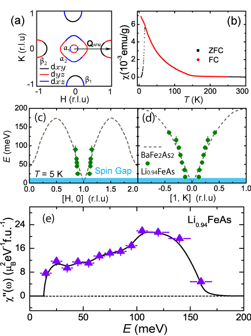
Our experiments were carried out on the ARCS time-of-flight chopper spectrometer at the spallation neutron source, Oak Ridge National laboratory. We also performed thermal triple-axis spectrometer measurements on the BT-7 triple-axis spectrometer at NIST center for neutron Research. Our single crystals were grown using the flux method and inductively coupled plasma analysis on the samples showed that the compositions of the crystals are Li0.94±0.01FeAs. Figure 1(b) shows zero field cooled (ZFC) and field cooled (FC) susceptibility measurements on Li0.94FeAs, which indicate spin glass behavior with no evidence for superconductivity. To study the spin excitations, we co-aligned 7.5 g of single crystals of Li0.94FeAs (with a mosaic of 2∘) and loaded the samples inside a He refrigerator or cryostat. To facilitate easy comparison with spin wave measurements in BaFe2As2 harriger , we defined the wave vector at (, , ) as reciprocal lattice units (rlu), where Å, and Å. For both triple-axis and ARCS measurements, we aligned crystals in the scattering zone. The ARCS data are normalized to absolute units using a vanadium standard. The incident beam energies were meV with parallel to the -axis.
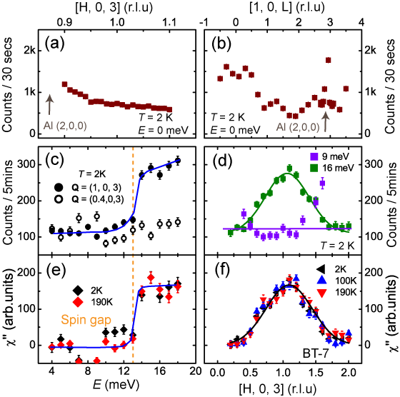
Before describing in detail the spin excitation dispersion curves and dynamic local susceptibility in Figs. 1 (c)-1(e), we first discuss the triple-axis measurements on the static AF order and spin excitations. Figures 1(a) and 1(b) show elastic scattering along the and directions across the expected AF peak position , respectively. In contrast to Na1-xFeAs, where static AF order is clearly observed slli , there is no evidence for static AF order in this sample. To search for AF spin excitations, we carried out constant- scans at the AF wave vector and background positions. The outcome in Fig. 2(c) shows a step-like increase in scattering above background for meV, clearly suggesting the presence of a large spin gap of meV. To confirm there is indeed a spin gap, we carried out constant-energy scans along the direction at and 16 meV as shown in Fig. 1(d). While the scattering is featureless at meV, there is a clear peak centered at at meV. Figure 3(e) shows temperature dependence of the imaginary part of dynamic susceptibility obtained by subtracting the background and correcting for the Bose population factor. Surprisingly, the spin gap has no observable temperature dependence between 2 K and 190 K, much different from the temperature dependence of the spin gaps in the (Ba,Sr,Ca)Fe2As2 family of materials matan ; zhaoprl ; rob , which disappear rapidly with increasing temperature. The weak temperature dependence of the dynamic susceptibility has been confirmed by constant-energy scans in Fig. 2(f), where at meV remains essentially unchanged from 2 K to 190 K.
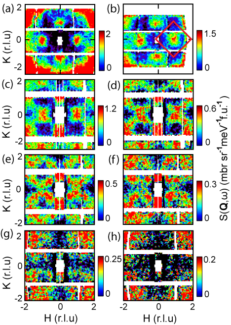

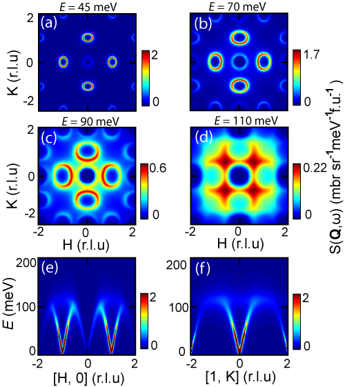
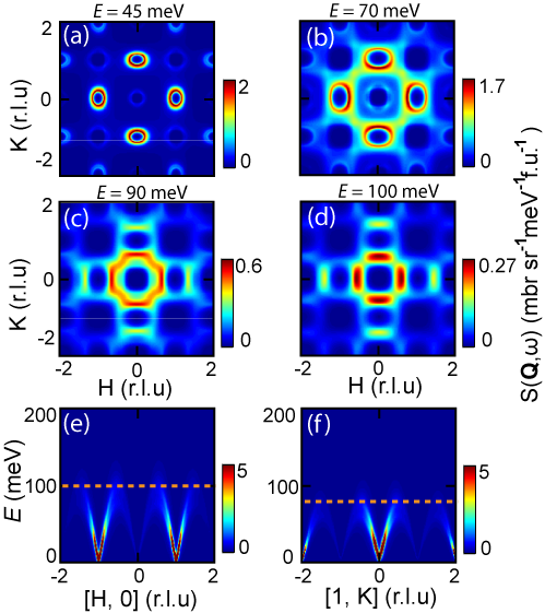
Figure 3 summarizes the ARCS time-of-flight measurements on Li0.94FeAs at 5 K. Since spin excitations in Li0.94FeAs have no -axis modulations, we show in Figs. 3(a)-3(h) two-dimensional constant-energy () images of the scattering in the plane for , , , , , , , and meV, respectively. For energies between meV, spin excitations form transversely elongated ellipses centered around AF . The intensity of spin excitations decrease with increasing energy, this is remarkably similar to spin waves in BaFe2As2 harriger . For energies above 90 meV, spin excitations split into two horizontal arcs that separate further with increasing energy. The excitations finally merge into () and become weaker above 150 meV in Fig. 3(g) and 3(h).
In order to determine the dispersion of spin excitations for Li0.94 FeAs, we show in Fig. 4 cuts through the two-dimensional images in Fig. 3 and compare with identical cuts for BaFe2As2. Figures 4(a)-4(d) show constant-energy cuts along the direction for energies of , , , meV, respectively, while the dashed lines show identical spin wave cuts for BaFe2As2 harriger . Since both measurements were taken in absolute units, we can see that spin excitations in Li0.94 FeAs are similar to that of BaFe2As2 per Fe below 95 meV harriger . Figures 4(e)-4(h) show constant-energy cuts along the direction for identical energies as that of Figs. 4(a)-4(d). For energies above 95 meV, the strength of the spin excitations in Li0.94FeAs are rapidly suppressed compared to those of BaFe2As2 and become very weak above meV. This can originate from an absence of magnetic scattering, or that the scattering is very broad as might occur when an itinerant electron system interacting with Stoner excitations. This is different from spin waves in BaFe2As2, which extend up to 250 meV. Based on these constant-energy cuts, we show in Figs. 1(c) and 1(d) the comparison of spin excitation dispersions of Li0.94FeAs (filled circles) with those of spin waves in BaFe2As2 (dashed lines). They are similar for energies between meV, while the spin excitations in Li0.94FeAs are broader below 50 meV.
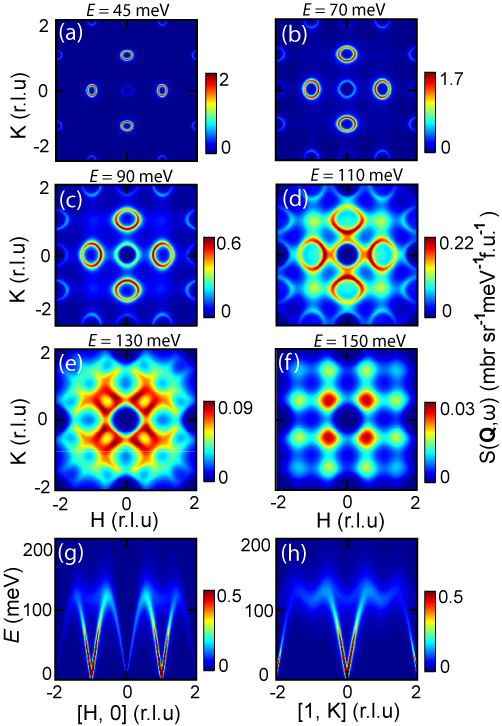
We have attempted, but failed, to use a simple Heisenberg Hamiltonian with the effective nearest and next nearest neighbor exchange couplings to fit the observed spin excitations spectra harriger ; jzhao . For all the possible combinations of the , , and , the expected zone boundary spin excitations are quite different from the observed spectra (see supplementary information) suppl . If we include the next-next nearest neighbor exchange coupling , the expected spectra near the zone boundary have some resemblance to the data in Fig. 3 although the low-energy excitations would be different (see supplementary information). This means that the effective exchange couplings in Li0.94FeAs are extremely long-ranged, a hallmark that itinerant electrons are important for spin excitations in this material. Since the data close to the band top along the direction are higher in energy than along the direction, we need to recover this feature in a --- model (see supplementary information). This means that effective exchange interactions in Li0.94FeAs may be similar to the (Ca,Sr,Ba)Fe2As2 iron pnictides harriger ; jzhao ; ewings in spite of their different zone boundary spectra.
Finally, we show in Figure 1(e) the energy dependence of the local susceptibility, defined as , where the average is over the magnetic scattering signal over the Brillouin zone [Fig. 3(b)] lester . The corresponding fluctuating moment per formula unit. We can use both pure local and itinerant spin models to sketch a basic physical picture based on the moment value. If we assume a quantum local spin model to describe the fluctuations, the moment value implies the spin value is about one. If we take a pure itinerant model, our result would suggest that at least three electrons per iron site occupy the states with energies up to the magnetic bandwidth ( meV) below the Fermi energy. This suggests that the bandwidths of the electron bands near the Fermi surface are extremely narrow. In other words, the band renormalization factors are large and the electron-electron correlations must be strong.
In summary, we measured spin excitations in single crystals of Li0.94FeAs. Similar to other iron pnictides, the low energy excitations are still strongly AF platt . However, comparing to other iron pnictides, they have several distinct properties: (a) a larger spin gap, close to meV that is essentially temperature independent below 190 K; (b) a comparable total magnetic bandwidth; (c) different wave vectors at the zone boundary for high energy excitations. Moreover, the excitations can not be described by magnetic models with only short range magnetic exchange couplings. Our results suggest the AF spin fluctuations are fundamental to the superconductivity of FeAs-based materials. FM fluctuations exist in Li0.94FeAs, but they only affect the high energy spin excitations.
During the process of writing up this paper, we became aware of a related work on powder samples of superconducting LiFeAs, where AF spin fluctuations have been reported taylor .
The work in IOP is supported by CAS, the MOST of China and NSFC. This work is also supported by the U.S. DOE BES No. DE-FG02-05ER46202, and by the U.S. DOE, Division of Scientific User Facilities.
References
- (1) D. C. Johnston, Adv. in Phys. 59, 803 (2010).
- (2) M. D. Lumsden and A. D. Christianson, J. Phys.: Condens. Matter 22, 203203 (2010).
- (3) J. W. Lynn and P. C. Dai, Physica C 469, 469 (2009).
- (4) Y. Kamihara et al., J. Am. Chem. Soc. 130, 3296 (2008).
- (5) C. de la Cruz et al., Nature (London) 453, 899 (2008).
- (6) I. I. Mazin et al., Phys. Rev. Lett. 101, 057003 (2008).
- (7) J. Dong et al., EPL 83, 27006 (2008).
- (8) H. Ding et al., EPL 83, 47001 (2008).
- (9) K. Seo et al., Phys. Rev. Lett. 101, 206404 (2008).
- (10) K. Kuroki et al., Phys. Rev. Lett. 101, 087004 (2008).
- (11) A. V. Chubukov, Physica C 469, 640 (2009).
- (12) F. Wang et al., Phys. Rev. Lett. 102, 047005 (2009).
- (13) X. C. Wang et al., Solid State Commun. 148 , 538 (2008).
- (14) J. H. Tapp et al., Phys. Rev. B 78, 060505(R) (2008).
- (15) M. J. Pitcher et al., Chem. Commun., 5918 (2008).
- (16) F. L. Pratt et al., Phys. Rev. B 79, 052508 (2009).
- (17) C. W. Chu et al., Physica C 469, 326 (2009).
- (18) S. V. Borisenko et al., Phy. Rev. Lett. 105, 067002 (2010).
- (19) P. M. R. Brydon et al., Phys. Rev. B 83, 060501(R) (2011).
- (20) O. J. Lipscombe, et al, Phys. Rev. Lett. 106, 057004 (2011).
- (21) L. W. Harriger et al., arXiv: 1011.3771.
- (22) J. Zhao et al., Nat. Phys. 5, 555 (2009).
- (23) R. A. Ewings et al., arXiv: 1011.3831.
- (24) S. L. Li et al., Phys. Rev. B 80, 020504(R) (2009).
- (25) K. Matan et al., Phys. Rev. B 79, 054526 (2009).
- (26) J. Zhao et al., Phys. Rev. Lett. 101, 167203 (2008).
- (27) R. J. McQueeney et al., Phys. Rev. Lett. 101, 227205 (2008).
- (28) See supplementary information for details.
- (29) C. Lester et al., Phys. Rev. B 81, 064505 (2010).
- (30) C. Platt, R. Thomale, and W. Hanke, arXiv: 1103.2101v1.
- (31) A. E. Taylor et al., arXiv: 1104. 1609v1.
Supplementary Information: Antiferromagnetic spin excitations in single crystals of
nonsuperconducting Li0.94FeAs
Meng Wang, X. C. Wang, D. L. Abernathy, L. W. Harriger, H. Q. Luo, Yang Zhao, J. W. Lynn, Q. Q. Liu, C. Q. Jin, Chen Fang, Jiangping Hu, Pengcheng Dai
Meng Wang
X. C. Wang
D. L. Abernathy
L. W. Harriger
H. Q. Luo
Yang Zhao
J. W. Lynn
Q. Q. Liu
C. Q. Jin
Chen Fang
Jiangping Hu
Pengcheng Dai
In order to test if a simple --- Heisenberg Hamiltonian can reproduce the observed spin excitations spectra in Fig. 3, we simulated the expected spin wave spectra using Heisenberg Hamiltonian jzhao . To facilitate direct comparison with the data in Fig. 3, we normalized the calculated intesity at 90 meV to be the same as that in Fig. 3. Therefore, the calculated spectra can be directly compared with the observed spectra. Figure SI5 shows spin wave calculations assuming meV, meV, meV, and meV. While the zone boundary spectra have some similarity to the data, the spectra clearly disagree with the data around intermediate energies. Figure SI6 shows similar calculation assuming meV, meV, and meV. Figure SI7 plots calculations assuming meV, meV, meV, and meV; and Figure SI8 show calculation with meV, meV, and meV. The spin wave band tops are in Figs. SI5-SI8 are 150 meV, 150 meV, 110 meV, and 100 meV, respectively. To obtain similar scattering pattern as observed near the band top by a Heisenberg Hamiltonian with effective exchange couplings, the next-next nearest neighbor exchange coupling has to be included.
We note that spin excitations close to the band top in Fig1(e) clearly shows that zone boundary energy in the direction is higher in energy than that along the direction. In the following we show that in a --- model with antiferromagnetic and and ferromagnetic , we need and only need (ferromagnetic) to recover this feature.
The --- model is analogous to the -- spin model used to describe CaFe2As2jzhao . In the following we will consider a detwinned system, and one should bear in mind that one q-point in a twinned system corresponds to and in a detwinned one. The spinwave dispersion for this model is given by
| (1) |
where
| (2) | |||||
In the model, the dispersion along -direction sees the maximum at , while along -direction, the maximum is at where is in fact parameter dependent. But one should not only compare and to find which direction reaches a higher top, because there is twinning. Once we have twinning into play, we also need to compare the band near . Mark that in discussing this region, and directions should be interchanged when compared with the experimental frame. Starting from , the dispersion reaches maximum along -direction at and along direction at . Therefore, in order to see what we see in the experiment, we should have
| (3) |
Now we make a statement and prove it: is sufficient and necessary for the Eq.(3) to hold. First we prove the sufficiency.
| (4) |
From this we know if , we have . On the other hand,
| (5) |
From this we know if
| (6) |
. But of course
| (7) |
therefore is sufficient to make the highest energy along direction higher than direction.
Then we prove the necessity. It is a proof by contradiction. Suppose , then from above we know that . Also notice that when ,
Therefore
| (9) |
Therefore we have proved if then the highest energy along direction is lower than the highest energy along direction, i.e., is necessary to recover the feature observed in experimental data.

References
- (1) J. Zhao et al., Nat. Phys. 5, 555 (2009).