Isolating CP-violating coupling in with transverse beam polarizations
Abstract
We revisit the process at the ILC with transverse beam polarization in the presence of anomalous CP-violating coupling and coupling . We point out that if the final-state spins are resolved, then it becomes possible to fingerprint the anomalous coupling Re. 90% confidence level limit on Re achievable at ILC with center-of-mass energy of 500 GeV or 800 GeV with realistic initial beam polarization and integrated luminosity is of the order of few times of when the helicity of is used and when the helicity of is used. The resulting corrections at quadratic order to the cross section and its influence on these limits are also evaluated and are shown to be small. The benefits of such polarization programmes at the ILC are compared and contrasted for the process at hand. We also discuss possible methods by which one can isolate events with a definite helicity for one of the final-state particles.
pacs:
13.66.-a, 12.60.-i, 13.88.+eI Introduction
The International Linear Collider (ILC) [1, 2] is a proposed collider that will collide electrons and positrons at high energy and luminosity and is expected to verify the predictions of the standard model (SM) at a high level of precision, and to establish interactions beyond the SM even if there is no direct production of particles that are not in the spectrum of the SM. One window to such new physics is the discovery of CP violation beyond what is predicted by the SM; for a review on basic principles of CP violation at colliders, see Ref. [3]. It has been shown that the availability of beam polarization of one or both of the beams, transverse and longitudinal, can significantly enhance the sensitivity to such beyond the SM interactions; see, e.g., Ref. [4] for a recent review.
If beyond the SM interactions are very subtle, then it is particularly important to search for deviations from the SM to linear order. Keeping these considerations in mind, the issue of sensitivity to linear order of CP-violating anomalous gauge boson couplings, denoted by () and () to be defined later, that contribute to the process with longitudinal beam polarization was considered in Ref. [5], and with transverse beam polarization in Ref. [6] (for earlier discussions in the context of unpolarized beams see Ref. [7, 8, 9], and Ref. [10] for beam polarization effects). These couplings are absent in the SM even at loop level, and can be thought of representing some basic interactions arising from an underlying theory; for instance they can arise in some extensions of the SM at the one-loop level [11, 12, 13, 14], and thus their nonvanishing value indicates a signature of new physics. Anomalous couplings have been investigated at the Large Electron Positron (LEP) collider, resulting in limits of the order of 0.05 (0.13) on the magnitude of () couplings [15]. The most stringent bounds on the absolute value of these couplings comes from the recent D0 and CDF Collaboration results of Tevatron [16, 17]. Apart from these direct limits, imposing unitarity of partial wave scattering amplitudes can give limits on the couplings [8, 18]. For an ILC operating at GeV, the analysis of Czyz et al. [18] gives the unitarity limits . Other unitarity limits are expressed as of the order of (0.1 TeV on dimension-6 couplings and of the order of ( TeV on dimension-8 couplings, where is the assumed scale of new physics [8]. A review of these results may be found in Ref. [19]. Considerations of the anomalous sector involving W bosons have also been recently studied in the context of the Large Hadron Collider, see Refs. [20, 21] and Ref. [22] for quartic couplings involving pairs along with W pairs as well as Z pairs and references therein.
Since, in the process at hand, - and -channel exchanges are present there is an additional dependence on the polar scattering angle () between and direction. A polar-angle forward-backward asymmetry is seen with longitudinally-polarized beams due to the interference of the CP-violating anomalous coupling with SM contribution [5], because the photon should be produced symmetrically if CP is conserved. Longitudinal beam polarization improves sensitivity to some of the form factors, whereas the transversely polarized beams with new combinations of polar and azimuthal asymmetries enable better measurement. This is due to the fact that with transverse beam polarization, one has an additional angle , the azimuthal angle with respect to the direction of quantization of the electron polarization, which allows one to obtain distributions that are sensitive to the real parts of the anomalous couplings. In order to obtain the fully differential cross sections in the presence of anomalous gauge couplings, one may use the helicity amplitudes listed in Ref. [18] and account for the transverse polarization using the generalized formalism of Ref. [23]. Suitable asymmetries may then be constructed which can be used to extract these anomalous couplings. Furthermore, one can obtain 90% confidence limits on these couplings if no signal is observed for realistic beam polarization and typical integrated luminosities. It may be emphasized that the limits obtained in this work are completely based on an analytical approach and is a strength of the method and is an extension of the approach of Ref. [6] which have proven necessary for the extraction of Re . It would be a useful benchmark for future simulation studies of the same system.
As a consequence of the CPT theorem, in the absence of beam polarization and with longitudinal beam polarization, only the imaginary parts of these contribute to the cross section at linear order. It turns out that with transverse beam polarization and due to the interference of the SM amplitudes with those arising from anomalous couplings, only Re contributes to the fully differential cross section, whereas the Re contribution vanishes because the photon has only vectorlike couplings. Thus the question of isolating to leading order remains open.
Recently, it was shown, in the context of production with beyond the SM interactions parametrized in terms of effective four-Fermi interactions, that the measurement of final-state helicity can help in disentangling the contributions of scalar and tensor like four-Fermi interactions when the beams are transversely polarized [24].
Inspired by the considerations in the work above, we now ask whether at leading order one can isolate by the measurement of the helicity of the or the photon. The answer is in the affirmative. Whereas the considerations of the top-quark helicity referred to above can be extended to the , which we describe in a little detail later on, there is no analogous method for determining the helicity of the photon as it is a stable particle. At low energies the final-state helicity determination is a key ingredient for the determination of neutrino helicity in the well-known Goldhaber experiment [25]. However, it is conceivable that there are materials that can be used in the construction of the ILC detectors which could be used for these determinations. In particular aligned crystals could be candidates for such detectors in case of high-energy photons, as has been considered by the NA59 collaboration[26]. Leaving aside the experimental question of measurement of the final-state helicities, which would affect the sensitivity, we construct asymmetries that involve, e.g., samples of positive and negative helicities, and also photon helicities. These are then translated into 90% confidence limits on the anomalous couplings by combining them with the previously established results. The best limits are expressed in the - plane. If these are set to zero one at a time, then we obtain the limit on to be 0.0958 when the helicity of only the is resolved for a total center-of-mass energy (c.m.) of 500 GeV with an integrated luminosity of 500 fb-1 and realistic polarizations. An improved limit of is obtained when the helicity of is resolved. The stability of these limits when they are fed back into the expressions at quadratic order for the cross section is also addressed, by iteratively including the effects which turn out to be not of great significance in practice.
This paper is organized as follows: In Sec. II, we recall the basic vertices and present the definitions, followed by Sec. III, where we present the results of our computation of the fully differential cross section with final-state helicity resolution. In Sec. IV we define the asymmetries that we have used to obtain 90% confidence limits. In Sec. V we present a detailed discussion on the possibility of obtaining samples of define helicities and discuss the issue of photon and helicity measurement. In Sec. VI we present a summary of the results and a discussion.
II Formalism for the process
We begin by writing down the formalism for the process closely following the treatment in Ref. [6]. We consider the process
| (1) |
where can take values and the value for can be and 0. As in Ref. [6], we impose electromagnetic gauge invariance. The most general effective -violating Lagrangian, retaining terms upto dimension 6 can be written as [5]
| (2) |
where is the electric charge, is the mass of boson, and , with as the weak mixing angle. and are in general complex. Terms involving divergences of the vector fields have been dropped from the Lagrangian.
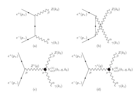
The SM diagrams contributing to the process (1) are shown in Figs. 1 (a) and 1 (b), which correspond to – and a –channel electron exchange, while the extra piece in the Lagrangian (2) introduces two –channel diagrams with – and –exchange, respectively, shown in Figs. 1 (c) and 1 (d). Here we have used as the momentum label for the intermediate state in the channel, and the tensors and corresponding to the three-vector vertices are given by
| (3) |
We have computed the cross section incorporating transverse beam polarization using the helicity amplitudes given in [18]. Note that the parametrization of the anomalous coupling, where or in [18] is given in terms of and . 111They are related to and as, and .
The cross section for the transversely polarized state can be expressed as [23]
where the and are helicity amplitudes for the process at hand, is the final-state azimuthal angle and is the unpolarized cross section. In , the subscripts stand for the helicities of the and respectively. In the above, beyond standard model (BSM) interactions of the chirality–conserving type contribute to the amplitudes and , while those of the chirality–violating type contribute to (the SM interactions themselves contribute only to and , when effects are neglected). Note also the characteristic dependence accompanying the terms bilinear in transverse polarization, and the dependence accompanying the linear transverse polarization pieces when the BSM physics is worked out to leading order.
However the process under study is of the annihilation type and contains no electron and electron neutrino in final state, so . So the above expression reduces to a much simplified form which is given below
| (4) |
This will be used in the following sections to evaluate the distributions of interest.
III Distributions in the presence of transverse polarization
We now give explicit expression for differential scattering cross section, for the two cases, viz., when the helicity of is resolved, summing over the helicity of , and vice versa.
Let us introduce the definitions :
where is the square of the total c. m. energy, and and represent the vector and the axial vector couplings of the electron with given by
| (6) |
In the equations below only terms of linear order in the anomalous couplings, are retained since they are expected to be small. So far as the CP-violating part of the differential cross section is concerned, this is not an approximation, since the only contribution is from the interference between the SM amplitude and the CP-violating amplitude, linear in the anomalous couplings. The denominator of the asymmetries which we calculate, however, would in principle receive a contribution from terms quadratic in the anomalous couplings. In principle, the validity of the linear approximation is dependent on the c. m. energy of the process, and for larger c. m. energy would require the couplings to be smaller. We will see that in our case the contribution of the quadratic terms to the cross section is negligible for Re and Re below about 0.01, where our limits lie, and therefore the linear approximation holds good. Expressed differently it can be said that the observables defined here are not sensitive to quadratic terms in the cross section, for the values which will be probed at the linear collider.
Resolving the polarization of and summing over the polarizations of , the differential cross sections for the production of circularly polarized and longitudinally polarized are given by
| (7) |
| (8) |
Here
| (9) |
are the corresponding SM differential cross sections, and we have defined
| (10) | |||||
and
| (11) |
Note the appearance of in . On summing over the helicities, however, the dependence on disappears. In the above, as defined earlier, is the angle between photon and the beam direction of , chosen as the axis. is the azimuthal angle of the photon with the direction of the transverse polarization of the chosen as the axis. is the integration measure for the angular variables and . The polarization direction can be parallel or antiparallel to the polarization direction, the polarization in the former case being taken as positive.
The cross sections for two circular polarization states of summing over all the states are given by:
| (12) |
where
| (13) | |||||
and
| (14) | |||||
Again, occurs in , but cancels on summing over the helicities.
Here one can easily check from Eq. (9) for Z and Eq. (13) for that after summing over different final helicity states we get the same result, which also agrees with one obtained in[6] for unpolarized final states.
At the ILC it is expected that about 90% electron polarization would be achievable along with a positron polarization of 60% [4]. The beams will be longitudinally polarized, but there is a possibility that spin rotators can be used to produce transversely polarized beams. and are, respectively, the degrees of polarization of the and ; for our calculation we have taken a realistic value of = 0.8 and = 0.6. In the next section we will employ these expressions to obtain 90% confidence level(CL) limits on .
IV Asymmetries and Numerical Results
In order to make the above expressions useful for applications at the ILC, and to disentangle the anomalous couplings, we will define certain asymmetries that will isolate with =1,2. Since the dependence of the new couplings on the laboratory observables such as polar and azimuthal angles are different, a suitable choice of asymmetries can help in achieving this goal. For the helicity–summed case, it was observed that the contribution from Re was zero. But the inclusion of helicity of either of the final-state results in a contribution from . Therefore the situation where all the spin configurations are available is explored in this section by constructing various asymmetries. A through numerical analysis is done to put a bound on the anomalous coupling along with .
IV.1 Integrated Asymmetries
We define two CP-odd asymmetries constructed from suitable partial cross sections. In all case, we assume a cut-off of on the polar angle in the forward and backward directions, required to stay away from the beam pipe, and our asymmetries are therefore functions of . The cut-off may be chosen to optimize the sensitivity. One of the asymmetries, , combines a forward-backward asymmetry along with an azimuthal symmetry. The other, , is an asymmetry only in . The asymmetries are given by
| (15) |
| (16) |
with the SM cross section given by
| (17) |
where V can be or depending on whose polarization is being considered. Since we are mainly concentrating on the coupling Re, from Eq. III we see that longitudinal with is not sensitive to this coupling. Therefore we will be mainly concentrating on with .
Here and are calculated for different combinations of which is the value obtained when the two helicity states of are summed over or the difference is taken.
| (18) |
| (19) |
Here refers to with helicity . The above choice of asymmetries is motivated by the purpose of isolating the couplings Re and Re. Equation (18) contains a term proportional to coming from , which with polar angle forward-backward asymmetry in survives, whereas goes to zero. Similarly Eq. (19) contains term independent of coming from , therefore the polar angle forward-backward asymmetry of is equal to zero, and survives. In this case the term proportional to coming from vanishes for both and .
-
1.
Considering the case when the helicity of is kept and that of is summed over:
-
2.
Now considering the case that helicity of is measured with that of summed over:
Analyzing Eqs. (1), (1), (2) and (2), it is seen that for both and , is only sensitive to Re, whereas depends on both Re, , where = , . The above is due to the polar angle dependent term in Eq. (18) surviving for , and the helicity dependent polar angle independent term in Eq. (19) surviving for . Comparing our results to the earlier work where all the three helicity states of are summed over [6], the same asymmetry evaluated for Eq. (18), for the two transverse states of is smaller by a factor of . Because of this the limit on Re is poorer in this case, whereas the additional advantage here is that we can put a limit on Re which was not possible earlier. The analysis done for the case of does not encounter this problem as here we are summing over all its helicity states, unlike the case of .
IV.2 Numerical Analysis
We have calculated the cross section and the asymmetries for the case when polarization is parallel to . For our sensitivity analysis, we have assumed an integrated luminosity of 500 .
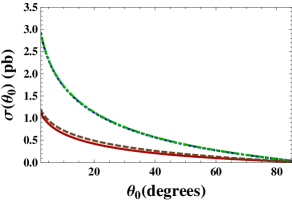

Figure 3 shows the total cross section , plotted as a function of cut off angle at = 500 GeV and 800 GeV. The anomalous couplings contribute to the total cross section only at quadratic order [5]. We have kept these terms in Fig. 3, for a particular combination. Similar behavior occurs for the case and , since the cross section is almost symmetric in and with almost equal to 1. It is clear from the figure that the contribution of anomalous couplings is negligible for values below 0.01, which correspond to the limits we find from asymmetries given later. The corresponding limits on Re are 0.0048 at Gev and 0.0014 at Gev for cut off angle = . The same limits will hold for Re piece. Later in this section, we will see that these limits are more stringent than the case but comparable to the case when the helicity of is considered. The total cross section receives contribution both from CP–conserving and CP–violating anomalous couplings. Therefore, measuring deviation of the total cross section from the SM prediction would not really be a test for CP–violating couplings which we are considering here. The linear contribution from the real part of the CP–violating couplings only occur in the case of transverse polarization and has no effect on the total cross section. The imaginary parts contribute in linear order to the differential cross section, but their effect is washed out in the total cross section after the integration.
We have done our whole numerical analyses for two different cases at of 500 and 800 GeV. In the first case, we drop the terms quadratic in anomalous couplings from the denominator of the asymmetries Eqs. (15), (16). The best limits on the couplings obtained in this case are of the order of . For the second case, we then include the terms quadratic in anomalous couplings to the denominator of Eqs. (15), (16) with the value coming from the best limit obtained in the earlier case. It is apparent from the above discussion that, this contribution of order in the denominator would not much affect the asymmetries and the limits obtained from them. This is another way of putting the argument that the asymmetries and the limits obtained are not sensitive to the quadratic terms in the denominator at the level in which they can be probed. We present the results in detail for the first case, i.e., without including quadratic terms, and then show the effect on inclusion of quadratic terms.
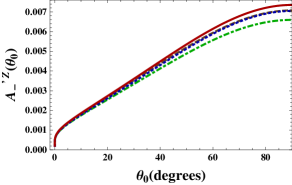

We now consider the case when the helicity of is resolved. Figure 3 shows the integrated version of the asymmetry plotted as a function of cut-off for different c.m. energies with a value of Re=0.1. Figure 5 shows as a function of cut-off , when the value of the anomalous couplings are taken as Re =0.1 and Re =0 for different c.m. energies. However, as mentioned before, Re, in the case of , is accompanied by the numerically small coefficient and thus we obtain a larger limit on Re where our linear approximation is not valid. So we will drop Re in our consideration of from here onwards. behaves differently from due to the presence of the term in the numerator. The asymmetry in the latter case increases with the cut off due to the SM cross section in the denominator which decreases faster than the numerator. In all the above cases the asymmetry does not change much with c. m. energy as the observables above are all independent of it. We have not given the figure corresponding to since it has already been considered in Ref. [6]. The figures are all plotted with and without including quadratic terms in the denominator of Eq. (15), (16). It is observed that there is not much deviation, with the inclusion of quadratic terms couplings for the values, at the level probed by the linear collider.
A similar analysis follows for the case when the helicity of is resolved while that of is summed over. Figure 5 shows the integrated version of as a function of cut-off , when the values of the anomalous couplings are taken as Re =0.1 and Re =0 for different c.m. energies. The behavior is the same as that of the case when helicity of is resolved except the fact that here the asymmetries are enhanced by an extra factor of about 30 at =500 GeV and a factor of about 75 at =800 GeV due to the presence of the term in the numerator of Eq. (2). Because of this boost factor we get limit on Re which is well under the ambit of linear approximation and thus we will retain it for further consideration in . Moreover due to the presence of this enhancement term, the asymmetry is sensitive to c.m. energy. In this case also the asymmetries and the limits are calculated with and without including quadratic terms in the denominator.
The asymmetries are used to calculate 90% CL limits with realistic integrated luminosities in the absence of any signal at ILC. The limit on the coupling is related to the value of the asymmetry by:
| (26) |
where is the number of SM events and A is the value of the asymmetry for unit value of the coupling. The coefficient 1.64 may be obtained from statistical tables for hypothesis testing with one estimator; see, e.g., Table 33.1 in Ref. [19].
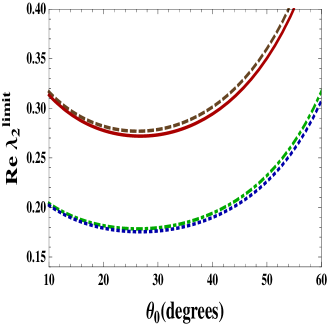
We see from Eqs. (1) and (2) that solely depends on Re, therefore an independent limit can be placed on it. Considering the helicity of , Fig. 6 shows that the best limit for Re from is obtained for = at = 500 GeV, though any nearby values of will give the same results. The limit corresponding to Re is 0.1757. A poor limit is obtained for = 800 GeV, as the SM cross section in the denominator of Eq. (26) decreases much faster with the c.m. energy compared to the asymmetry, which does not change. This can be understood much more clearly from Eqs. (1) and (1), where the anomalous couplings are not sensitive to the c.m. energies for the transversely polarized . Similar analysis is carried out for . Since depends on Re, Fig. 8 shows that the best limit on Re is obtained for = at = 500 GeV. The limit on for Re is 0.0958. The limits obtained do not change much with the inclusion of quadratic terms.


The results obtained on repeating the earlier analysis for the case when the helicity of the is resolved, for different c. m. energies, is shown in Figure 8. In this case the sensitivity improves with c. m. energy. This is in contrast to the case where the helicity of is resolved, as from Eq. (26), the SM cross section, which decreases with the c.m. energy, is compensated by the asymmetry , which increases much more rapidly with energy, due to the term . This also explains the better limits obtained on the couplings in this case. The best limit is obtained for = with Re = 0.0033 at = 500 GeV whereas for = 800 GeV, the limits improve to Re = 0.0020 for = .
We have also evaluated the simultaneous 90% CL limits that can be obtained on Re and Re from and for the case . In case of , the numerator in Eq. 2 is accompanied by a factor , resulting in an enhancement. The region enclosed by the contours obtained by equating the asymmetry with Re as well as Re simultaneously nonzero to corresponds to the region allowed at the 90 % CL. The coefficient 2.15 may be obtained from statistical tables for hypothesis testing with two estimators, see, e.g., Table 33.2 in Ref. [19].

The above equation is solved for the value of giving the best limit for the couplings, which for is , and similarly for we take as at = 500 GeV. Whereas at = 800 GeV, the best limits for the couplings are obtained at for and for . Figure 9 shows the simultaneous limit obtained on Re taking the helicity of , for = 500 GeV and 800 GeV. The individual limits obtained by taking one coupling to be nonzero at a time as well as the simultaneous limit on the anomalous couplings from the asymmetries for different c.m. energies are shown in Tables. 1 and 2. It is seen that a better individual limit is obtained on Re, compared to the simultaneous limit. On the other hand, the simultaneous limit on Re is better than than the individual limit obtained on it from the asymmetry . This is due to the fact that the coefficient accompanying Re is too small, Eq. (2), to give a deviation from standard model results. But gives a better individual limit on Re compared to the simultaneous case as here the accompanying term is much larger compared to , Eq. (2).
| Coupling | Individual limit from | Simultaneous limits | |
|---|---|---|---|
| Re | |||
| Re | |||
| Coupling | Individual limit from | Simultaneous limits | |
|---|---|---|---|
| Re | |||
| Re | |||
V Utilizing Final-State and Helicities
In this section we discuss how the final-state helicities of the and the can be utilized in practice. We begin by discussing the case of the helicity of the . The discussion closely parallels the discussion that was recently provided for measuring the helicity of the top-quark in production given in Ref. [24]. So far we have assumed that it would be possible to isolate a sample of events where the has a definite helicity, which in practice is not possible as one can only measure polarization at a statistical level. Unlike an incoming beam of particles, which can be prepared in a pure spin state, an outgoing particle is not available in a pure state, but only a mixed state, yielding only an average polarization. In order to be able to make use of the definitions of various asymmetries which we discuss, we propose a practical method which would serve to provide a sample with predominantly positive or negative Z helicities, which would lead to a depletion of the efficiency, but would be able to achieve the main objective.
The spin of an unstable particle like the can be analyzed by looking at the distribution of its decay products. The decay distribution of a lepton produced from a with a definite helicity in the rest frame of the is given by
| (27) |
| (28) |
where is the angle made by the momentum of the with the spin quantization axis of the . The quantity which differentiates between the positive and negative helicity distributions is
| (29) |
For an elementary derivation of this result, see Sec. 10.2 in ref. [27].
It is thus seen from Eqs. (27), (28) that the tends to be emitted dominantly in the backward direction relative to the spin of the for transverse polarization, and peaks at for longitudinal polarization. Thus, by applying a cut keeping dominant emission of the fermions in the direction of the boost of the , one can obtain a sample which is enriched in events with negative helicity. Similarly, a cut keeping dominantly backward emission will yield a sample enriched in events with positive helicity. Finally, keeping leptons emitted mostly in the transverse direction will give a sample with dominantly zero helicity.
Thus, one has to actually generate events including decay and use the formulas to make predictions, and then compare the expected number of events for a given set of anomalous couplings with experiment and then place a limit. Such a procedure would give limits which are less stringent than obtained in our analysis. Strictly speaking, we should include full spin density matrices for production as well as decay into a certain final state, and consider asymmetries constructed out of the momenta of the decay products. However, we expect that the procedure described here will approximate such a complete description, with some reduction of efficiency.
To get some quantitative idea of the efficiency, we note that if we use the three charged-lepton channels for decay, with a combined branching ratio of about 10%, with the simplifying assumption that the -pair detection efficiency is 1, the sensitivity is a factor of of less. The inclusion of a channel would improve the sensitivity somewhat. A full analysis including decay entails a more complicated analysis with a different final state, and is beyond the scope of this work.
For projecting the final-state helicity, there is no analogous method, as it is stable. In the context of the Goldhaber neutrino helicity experiment [25], photons of a particular helicity were filtered out by the means of a magnetic material. Depending on the helicity state, photons are either absorbed in the material or not. Thus, by counting the events in the photopeaks observed with the scintillation detector for two different polarizations of the magnet, they determined the photon helicity. Here also one can conceive of using such a material in the construction of the ILC detector which could be used for polarization determination. We note here that, in the context of photon polarimetry measurements, it has been demonstrated by the CERN NA59 collaboration[26] that an aligned-crystal technology can be used for an accurate measurement of the polarization of initial-state photons in polarized photon collisions at high energies typical of the photon-photon collision mode of the ILC. Thus, it is conceivable that such technology could be extended to the needs of a detector that would seek to resolve the final-state photon helicity. We therefore advocate the construction of such photon helicity filtering detectors at the ILC that can open up the possibility of further improving the bound on Re.
VI Summary and Discussion
In this paper, we have studied the process at the ILC at = 500 GeV and 800 GeV with a realistic integrated luminosity. We have pointed out the benefits of the resolution of final-state spin for studying the effects of couplings which were otherwise invisible with initial longitudinal as well as transverse states. Inspired by the work of final-state top-spin measurement we have shown that one can isolate in the above process with initial transverse states by the measurement of the helicity of the or the photon.
We have also made a numerical study of the limits on various couplings that could be obtained at a future linear collider assuming realistic transverse polarizations of 80% and 60% respectively for and , respectively. We have also given the contour plot for allowed region in - plane. We see that with final-state spin resolution, transverse polarization can provide a sensitive test of the anomalous coupling, Re. Overall it is seen that the resolution of helicity of gives better limits on the couplings compared to the case when the helicity of is resolved. The above is due to the fact that only transversely polarized is sensitive to Re, but its contribution is smaller by a factor of . Moreover the contribution of Re and Re to the asymmetries and is inversely proportional to . Therefore in the case = 800 GeV the resolving power of asymmetries using the helicity of the is suppressed compared to the case when the helicity of is resolved. Since the anomalous couplings and cannot be completely disentangled through helicity measurements we present both simultaneous and individual limits where the latter is obtained by setting one of the couplings to zero at a time. These limits are found to be stable, when fed back into the expressions to quadratic order for the cross section. The asymmetries and the limits on the couplings are also calculated with the inclusion of quadratic terms for the cross section. The new limits obtained are summarized in Tables 1 and 2.
It must, however, be mentioned that one cannot directly isolate events with helicities of or . Hence to measure the asymmetries we discuss, one would have to carry out a subtraction of events in two kinematic regions of the decay products corresponding to positive and negative polarizations of the . Doing so would entail a loss of efficiency to a certain extent. We have not taken this into account. It may be possible to consider the cases when the helicities of as well as can be resolved. Indeed, the technology with aligned crystals, see Ref. [26] could be adapted for the final-state photon helicity resolution. It may be possible to carry out a study based on this, but is beyond the scope of the present work, as the features that we wish to study are already apparent when we sum over the helicity of one of the other. Furthermore, measuring both spins would lead to a loss in statistics thereby making this option less attractive. Additional studies beyond the scope of the present work are related to polarimetry.
We conclude by discussing some further approaches of value to the process at hand. It has been proposed that the hard radiative decay of the can also be used to place bounds on the magnitude of anomalous CP-violating couplings [28]. Of special significance is the construction presented in Refs. [29, 30] of the formalism of a general spin-1 density matrix for the -boson spin orientation introduced in the context of CP–conserving anomalous couplings. It would be of interest to see if this can be extended to the case of CP–violating anomalous couplings and so explore the possibility of using this formalism to obtain bounds on such couplings as we have done here. In Refs. [31, 32], the process has been studied with BSM interactions given by most general contact interactions with the helicities of the and summed over. It may be of interest to apply the present considerations to this scenario as well.
Acknowledgements: BA thanks the Department of Science and Technology, Government of India, and the Homi Bhabha Fellowships Council for support. SDR thanks the Department of Science and Technology, Government of India, for support under the J.C. Bose National Fellowship program, grant no. SR/SB/JCB-42/2009.
References
- [1] J. Brau et al. [ILC Collaboration], arXiv:0712.1950 [physics.acc-ph].
- [2] G. Aarons et al. [ILC Collaboration], arXiv:0709.1893 [hep-ph].
- [3] S. D. Rindani, Pramana 45, S263 (1995) [arXiv:hep-ph/9411398].
- [4] G. Moortgat-Pick et al., Phys. Rept. 460, 131 (2008) [arXiv:hep-ph/0507011].
- [5] D. Choudhury and S. D. Rindani, Phys. Lett. B 335, 198 (1994) [arXiv:hep-ph/9405242].
- [6] B. Ananthanarayan, S. D. Rindani, R. K. Singh and A. Bartl, Phys. Lett. B 593, 95 (2004) [Erratum-ibid. B 608, 274 (2005)] [arXiv:hep-ph/0404106].
- [7] K. Hagiwara, R. D. Peccei, D. Zeppenfeld and K. Hikasa, Nucl. Phys. B 282, 253 (1987).
- [8] U. Baur and E. L. Berger, Phys. Rev. D 47, 4889 (1993).
- [9] G. J. Gounaris, J. Layssac and F. M. Renard, Phys. Rev. D 61, 073013 (2000) [arXiv:hep-ph/9910395].
- [10] F. M. Renard, Nucl. Phys. B 196, 93 (1982).
- [11] D. Choudhury, S. Dutta, S. Rakshit and S. Rindani, Int. J. Mod. Phys. A 16, 4891 (2001) [arXiv:hep-ph/0011205].
- [12] G. J. Gounaris, J. Layssac and F. M. Renard, Phys. Rev. D 67, 013012 (2003) [arXiv:hep-ph/0211327].
- [13] G. J. Gounaris, J. Layssac and F. M. Renard, arXiv:hep-ph/0207273.
- [14] G. J. Gounaris, J. Layssac and F. M. Renard, Phys. Rev. D 62, 073013 (2000) [arXiv:hep-ph/0003143].
- [15] J. Alcaraz et al. [ALEPH, DELPHI and L3 Collaborations], arXiv:hep-ex/0612034.
- [16] V. M. Abazov et al. [D0 Collaboration], Phys. Rev. Lett. 102, 201802 (2009) [arXiv:0902.2157 [hep-ex]].
- [17] T. Aaltonen et al. [CDF Collaboration], Phys. Rev. D 82, 031103 (2010) [arXiv:1004.1140 [hep-ex]].
- [18] H. Czyz, K. Kolodziej and M. Zralek, Z. Phys. C 43, 97 (1989).
- [19] K. Nakamura et al. [Particle Data Group], J. Phys. G 37, 075021 (2010).
- [20] O. Kepka, C. Royon, Phys. Rev. D78, 073005 (2008). [arXiv:0808.0322 [hep-ph]].
- [21] E. Chapon, C. Royon, O. Kepka, Phys. Rev. D81, 074003 (2010). [arXiv:0912.5161 [hep-ph]].
- [22] J. de Favereau de Jeneret, V. Lemaitre, Y. Liu, S. Ovyn, T. Pierzchala, K. Piotrzkowski, X. Rouby, N. Schul et al., [arXiv:0908.2020 [hep-ph]].
- [23] K. i. Hikasa, Phys. Rev. D 33, 3203 (1986).
- [24] B. Ananthanarayan, M. Patra and S. D. Rindani, Phys. Rev. D 83, 016010 (2011) [arXiv:1007.5183 [hep-ph]].
- [25] M. Goldhaber, L. Grodzins and A. W. Sunyar, Phys. Rev. 109, 1015 (1958).
-
[26]
See talk by G. Ünel, 2010 at U. California, Irvine
http://thm.ankara.edu.tr/uphuk/4/s-pdf/unel-na59.pdf - [27] P. Renton, Electroweak Interactions: An Introduction to the Physics of Quarks and Leptons, Cambridge University Press, 1990
- [28] M. A. Perez and F. Ramirez-Zavaleta, Phys. Lett. B 609, 68 (2005) [arXiv:hep-ph/0410212].
- [29] I. Ots, H. Uibo, H. Liivat, R. Saar and R. K. Loide, Nucl. Phys. B 702, 346 (2004).
- [30] I. Ots, H. Uibo, H. Liivat, R. Saar and R. K. Loide, Nucl. Phys. B 740, 212 (2006).
- [31] B. Ananthanarayan and S. D. Rindani, Phys. Lett. B 606, 107 (2005) [arXiv:hep-ph/0410084].
- [32] B. Ananthanarayan and S. D. Rindani, JHEP 0510, 077 (2005) [arXiv:hep-ph/0507037].