Spitzer IRAC Low Surface Brightness Observations of the Virgo Cluster

Abstract

We present 3.6 and 4.5 µm Spitzer IRAC imaging over 0.77 square degrees at the Virgo cluster core for the purpose of understanding the formation mechanisms of the low surface brightness intracluster light features. Instrumental and astrophysical backgrounds that are hundreds of times higher than the signal were carefully characterized and removed. We examine both intracluster light plumes as well as the outer halo of the giant elliptical M87. For two intracluster light plumes, we use optical colors to constrain their ages to be greater than 3 & 5 Gyr, respectively. Upper limits on the IRAC fluxes constrain the upper limits to the masses, and optical detections constrain the lower limits to the masses. In this first measurement of mass of intracluster light plumes we find masses in the range of $5.5\times 10^{8}-4.5\times 10^{9}$ and $2.1\times 10^{8}-1.5\times 10^{9}$ M_⊙ for the two plumes for which we have coverage. Given their expected short lifetimes, and a constant production rate for these types of streams, integrated over Virgo’s lifetime, they can account for the total ICL content of the cluster implying that we do not need to invoke ICL formation mechanisms other than gravitational mechanisms leading to bright plumes. We also examined the outer halo of the giant elliptical M87. The color profile from the inner to outer halo of M87 (160 Kpc) is consistent with either a flat or optically blue gradient, where a blue gradient could be due to younger or lower metallicity stars at larger radii. The similarity of the age predicted by both the infrared and optical colors ($>$ few Gyr) indicates that the optical measurements are not strongly affected by dust extinction.

1 Introduction

The basic picture of hierarchical structure formation is that large galaxies assemble from smaller pieces. A galaxy’s environment during assembly is expected to play a significant role in its evolution. Indeed, galaxies in the dense cores of clusters differ systematically from those in the coeval field, in terms of their morphologies, stellar populations, and gas content (e.g. Dressler et al., 1997; Butcher & Oemler, 1978, 1984; Desai et al., 2007; Krick et al., 2009).

Many different physical processes have been implicated in driving the evolution of cluster galaxies, including both gravitational and gas dynamical effects. Gravitational effects include slow galaxy-galaxy interactions and mergers (Mihos, 2004), harassment (Moore et al., 1996, 1998), the effects of the global tidal field (e.g. Byrd & Valtonen, 1990; Henriksen & Byrd, 1996) and the effects of cluster sub-cluster merging (Bekki, 1999; Stevens et al., 1999). Gas dynamical effects include ram pressure and turbulent viscous stripping of the cold ISM (Gunn & Gott, 1972; Abadi et al., 1999; Schulz & Struck, 2001; Vollmer et al., 2001; Murphy et al., 2009) and starvation (Larson et al., 1980).

Within a cluster, gravitational effects can lead to the removal of stars from their parent galaxies into the intracluster medium (ICM). Gas dynamical effects can additionally strip gas and dust from galaxies. This stripped material may subsequently become sites of star formation within the ICM. The properties of these stars, as traced by the intracluster light (ICL), can constrain the types and frequency of the physical processes at work in clusters (Krick et al., 2006; Krick & Bernstein, 2007; Gonzalez et al., 2005; Feldmeier et al., 2004; Zibetti et al., 2005) by serving as a fossil record of the interaction history of the cluster.

Large stellar streams from galaxy interactions are a gravitational effect we know occurs in clusters. Massive streams will be visible for of order $\sim 1-2$ times their dynamical time before dispersing into the diffuse ICL population (Rudick et al., 2009). If the streams can account for all of the diffuse ICL built up over time, then there is no need to invoke other mechanisms such as gas dynamical effects including ram pressure stripping or starvation in generating large amounts of ICL.

Virgo is one of the best places to study these evolutionary processes in action. First, Virgo is the only cluster that is close enough (16.6 Mpc; Shapley et al., 2001) to easily achieve many resolution elements per square kiloparsec. Second, many of its galaxies have clearly been modified by their environment (Abramson et al., 2011). Third, the cluster exhibits substantial substructure, with infalling groups containing tidally interacting galaxies and mergers, as seen for the M87 & M86 regions (e.g. Schindler et al., 1999; Kenney et al., 2008). Finally, Virgo is well-studied at a range of wavelengths (there are at least 677 literature references in NED for the Virgo cluster).

As a central dominant (cD) galaxy of the Virgo cluster, M87 is a prototypical giant elliptical. Its optical surface brightness profile is poorly fit by a single deV profile; instead, better fits are achieved through high-n Sersic profiles (Kormendy et al., 2009; Janowiecki et al., 2010) or a combination of single deV profile with an additional outer component (Liu et al 2005). Either profile shape implies a significant amount of luminosity at large radius, possibly attributable to an ICL component. M87 is known to have a flat to slightly blue color gradient from the inside to outer regions of the galaxy (Liu et al., 2005; Zeilinger et al., 1993). A flat color profile implies a constant age as a function of radius. A color gradient, even in the near infrared, would imply changing age as a function of radius. Flat age profiles cannot rule out monolithic collapse scenarios for the formation of this giant elliptical .

At present, the only cluster-wide information obtained for the distribution of ICL in Virgo comes from the optical ($V\&B$-band) observations of Mihos et al. (2005) and Rudick et al. (2010). These data reveal an intricate complex of intracluster stellar features, including long ($>100$kpc) streamers, arcs, tails, bridges, and diffuse blobs unassociated with galaxies. These data are clear evidence for interactions between the infalling populations of smaller galaxies with the cluster cD (M87) and the infalling M86 sub-cluster structure.

In this paper we present a map of the central 0.77 square degrees in Virgo using IRAC at 3.6 and 4.5 µm. These wavelengths are interesting because they 1) are sensitive estimators of stellar mass, including that contributed by old stars; 2) will provide a color measurement of the diffuse features in this cluster; and 3) are largely unaffected by the presence of dust.

This paper is structured in the following manner. In §2 and §3 we discuss the data including specific reduction techniques for low surface brightness (LSB) measurements with Spitzer. Detection limits are described in §4. §5 discusses the results for the intracluster plumes and halo of M87. The paper is summarized and conclusions are drawn in §6. Throughout this paper we use $H_{0}=71$km/s/Mpc and $\Omega_{M}$ = 0.27. With this cosmology, we use the Shapley et al. (2001) luminosity distance of 16.6 Mpc corresponding to a redshift of 0.0039.

2 Spitzer Warm IRAC Observations

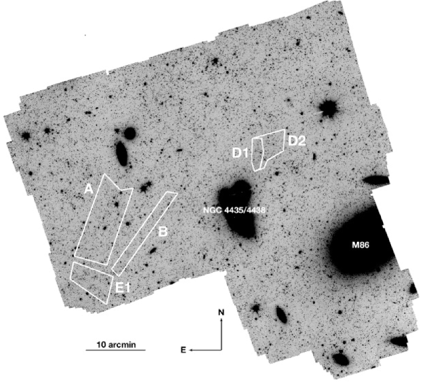
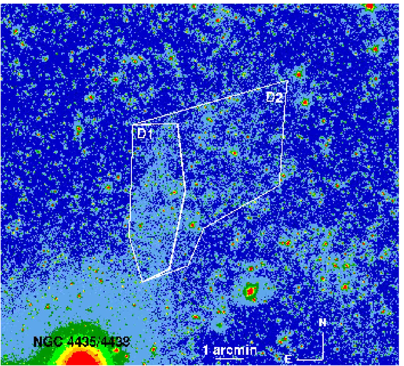
Figure 1: Top: The full 3.6 µm  mosaic, including intracluster and M87 halo regions as used in the text. Bottom: A zoom in on plume D where the low surface brightness signal is visible in the D1 region.

We make a continuous map of the central 0.77 square degrees of the Virgo cluster between M87 and M86 where many optical intracluster light features have been identified (Mihos et al., 2005; Rudick et al., 2009, see section §5.2 and Figure 1). We designed our observing program to reach the lowest possible surface brightness in the allotted time (100 hours; PID 60173). Our expected depth, based on the Spitzer sensitivity estimator, is 0.0002 Mjy/sr at 3.6 µm. Discrepancies from this will be discussed below. An additional design constraint was that the map include an “off” cluster region for measuring the non-cluster background level since we expect the diffuse intracluster light to be prevalent.

Warm IRAC (Fazio et al., 2004) simultaneously observes with two detectors at 3.6 & 4.5 µm  (channel 1 & 2 respectively). Each detector has a $5\farcm 2\times 5\farcm 2$ field of view with 1$\farcs$2 pixels. Images are acquired in two adjacent fields, separated by 6$\farcm$5. Our entire region is imaged in five layers of observations, each 10 min per pixel or 50 min per pixel total over all layers. Inside of each layer we dither inside of a mapping pattern to cover the entire area while facilitating the removal of cosmic rays. We use a 100 sec frame time which gives a coverage of at least 30 overlapping frames per pixel. 3.6 & 4.5 µm  data were taken simultaneously and so have similar coverage, except for one array width on the north and south side of the final mosaic. Data were taken during two consecutive, two week long, IRAC campaigns PC15 & PC16 during February, 2010. Due to scheduling constraints, the AORs are spread out in time between these two campaigns, i.e. they are not taken continuously in time.

3 Data Reduction

Data reduction to reach our intended low surface brightness detection limits is a challenge because it is a factor of hundreds below the background level in the images and very little work has been done to characterize the behavior of the IRAC instrument at these levels. The following sections discuss our data processing steps with an eye towards the errors in each step. We start with a standard data reduction for both channels. We use the Spitzer Science Center (SSC) pipeline which generates corrected basic calibrated data files (CBCD; pipeline version S18.18) for our data reduction. These data have already been dark and flat-field corrected with standard calibration darks and flat-fields. A flux conversion has already been applied based on A & K type standard stars placing the data in units of MJy/sr.

3.1 Dark & Bias Correction

Understanding the dark and bias contribution is important for LSB observations as it is a significant fraction of the total counts in each pixel. Calibration darks relevant to this dataset are taken as a set of 28 dithered 100s exposures within seven days of our observations. Standard darks can’t be taken with IRAC because the shutter is not ever used. The darks are taken by looking at a region of very low background near the north ecliptic pole. Those images are then median combined to remove sources which leaves an image of both the bias and dark current. Upon subtraction from the science data, both of these effects are removed. Because the dark field does not have a completely zero celestial background, this dark removal technique will also remove some real celestial background. We account for this in our program design by intentionally observing an “off” background location in the cluster which we will define to be of zero background, and tie the rest of the image to that (see §3.7).

3.2 Flat Field Correction

The accuracy of any LSB measurement is limited by fluctuations on the background level. A major contributor to those fluctuations is the large-scale flat-fielding accuracy. The IRAC flat-field is derived from dithered observations,accumulated over 110 hours, of the zodiacal background as the best approximation to a source which uniformly and completely fills the field of view. The pixel-wise accuracy of the flat-fields is very high, 0.2% & 0.1% at 3.6 & 4.5 µm  respectively. There is no variation with time in the flat field to the levels quoted.

3.3 Illumination Correction

There remains an illumination pattern in the science data in part due to latent images. Bright, saturated sources on prior images can fill traps in the arrays which decay away at a rate that is longer than the time between exposures thus leaving apparent flux at the location of that bright source in a previous image. Latent images can also result from the telescope slewing across a bright star which will leave a stripe of populated traps across the image. We removed these latents from the data by making a tailored illumination correction for each set of observations. In each individual CBCD, we mask all the detected sources based on a SExtractor (Bertin & Arnouts, 1996) segmentation map. SExtractor is run with a 1.5 sigma detection and analysis threshold and a minimum of 5 pixels for object detection. Then, the masked images are median combined inside of each observing set to create the illumination correction. Median combining these masked images does an excellent job of creating an illumination correction because there are of order 100 dithered images per channel. Because we only want to remove the pattern in this illumination image, and not the background level, we first subtract the mean level from the illumination image, then we subtract the illumination pattern from the science data.

3.4 Zodiacal Light Removal

The dominant, non-instrumental background source in space-based infrared observations is the zodiacal light. This is light scattered from interplanetary dust and depends on both time of year and direction of observation. The zodiacal light is assumed to be uniform on the size scale of the IRAC field of view. A single value of the zodiacal light per image is removed from the images using a model based on COBE DIRBE data (Kelsall et al., 1998) as listed in the headers. This model is expected to be accurate to 2% or better. Values for the zodiacal light are in the range of 0.104 to 0.114 MJy/sr at 3.6 µm  and 0.238 to 0.323 MJy/sr at 4.5 µm. Zodiacal light values are listed in the headers in units of MJy/sr. However the conversion from data units to MJy/sr provided by the Spitzer Science Center is based on point sources. Because the zodiacal light is an extended source, this point source derived conversion is not appropriate and we apply a multiplicative, extended source aperture correction to the zodiacal light value (0.91 and 0.94 at 3.6 & 4.5 µm respectively) before subtraction.

3.5 First Frame Effect

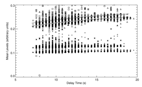
Figure 2: First Frame Correction: All $\sim 3000$ images at both 3.6 (squares+triangles) and 4.5 µm  (asterisks + pluses) are shown in this plot of delay time vs. mean background level. Mean levels have been arbitrarily scaled to show both channels on the same plot. The data from the two campaigns have different mean background levels as shown here with the different symbols within each channel. For the 3.6 µm  data the mean value in each bin of delay time is shown with the white asterisks which is then fitted with a logarithmic function shown by the solid lines.

The IRAC arrays are known to have a relation between the bias level and the delay time between frames. This is referred to in the documentation as the “first frame effect”, even though it effects all frames. Here, delay time refers to the time between one exposure and the next, and not the exposure time itself. There are different delay times between our images which all have the same exposure time because of the dithering and tiling pattern we have chosen. Figure 2 shows this effect for our dataset. Specifically, 3.6 µm data shows a logarithmic trend between bias level and delay time. The mean level shown is measured from masked individual CBCD frames that are column pulldown corrected. Masks are derived from SExtractor segmentation images. We fit the first frame effect separately for PC15 and PC16 with a logarithmic function and apply this as a correction to the data.

There is no measurable first frame effect in our 4.5 µm  data (see Figure 2). This is consistent with the known behavior of the arrays.

3.6 Clock Time Effect

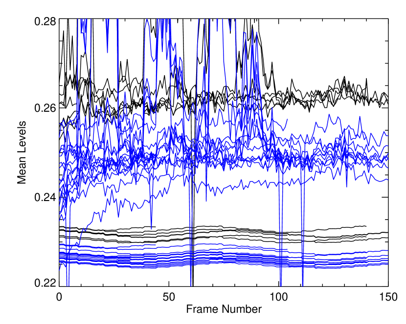
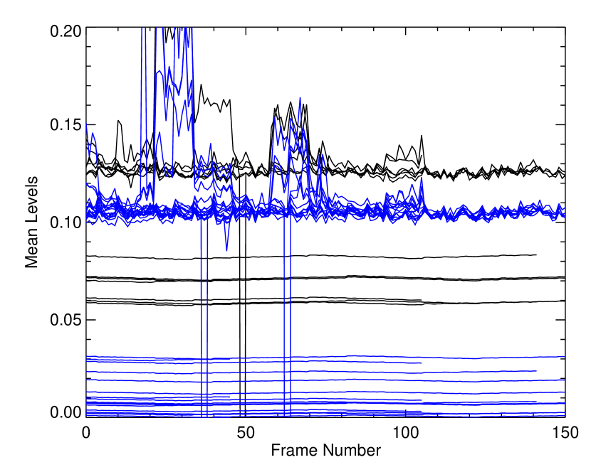
Figure 3: Relaxation effect for 3.6 µm (left plot) and 4.5 µm (right plot): Each of the 25 AOR’s is shown in this plot of frame number within the AOR vs. mean background level (arbitrary units) as solidly squiggly lines. AORs within campaign pc15 are shown in black, and those in campaign pc16 are shown in blue. Zodiacal light model levels are shown as smooth lines in the bottom third of the plot, arbitrarily scaled to fit in the frame. Spikes in mean level occur when a bright star or galaxy is on the frame. Our cycling dither pattern exposes some objects on multiple consecutive frames leading to spikes wider than one frame number.

After removal of the first frame effect, we notice a secondary, undocumented effect between mean levels and clock time at 3.6 µm. Figure 3 shows mean levels versus frame number for each of the 25 AORs as well as the zodiacal light model pattern for the same frames. Spikes in this plot occur when a bright star or bright galaxy are in the frame. There are two correlations: (1) a ramping in mean level from the beginning of the AOR to the end, and (2) mean level variation from AOR to AOR. We see a large jump in background levels between campaign PC15 data and campaign PC16 data, but also small level changes within the campaigns.

The zodiacal light pattern is not likely to be responsible for the ramping effect. This is demonstrated in the lower portions of Figure 3 where the zodiacal light contribution is shown. It has a significantly different shape than the ramping effect. Neither the jump or the ramp are correlated with position on the sky or time since dark frames were taken. This rules out astrophysical background and build-up of flux on the chip as causes of the effect.

It is likely that these effects are caused by the previous observation history of the chip. The ramping from the beginning to end of the AOR is likely a relaxation in the chip. As these AORs were not all taken sequentially in time, there is no way of knowing the precise observation history of the chips, and therefore no obvious correlations can be drawn with time since bright star observations or high background observations. The cause of the jump in background levels is unknown although potentially caused by zodiacal light model inaccuracies or previous observation history as with the ramping.

Because these effects can not be extragalactic in origin, we have chosen to remove them from the data. Each AOR trend is fit with an exponential function which is then subtracted from the data. We choose an exponential function as the appropriate model for a relaxation effect which fits the data well.

At 4.5 µm  there is the level change effect although not the ramping seen at 3.6 µm  (see Figure 3). Again, we remove the level change from the data to put all AOR’s on the same background level.

3.7 The Mosaic & Background Determination

After removal of the above discussed instrumental and zodiacal light effects, we use MOPEX (Makovoz & Marleau, 2005) for the final astrometry alignment and mosaicing, see Figure 1. M86 is marked for reference. M87 is in the lower left corner, not imaged in our survey.

We determine a global background level from the northern edge of the mosaic as an off-cluster region so that we can have an absolute measure of ICL flux in cluster regions. This assumes we have taken care of all instrumental and local celestial effects, and the only remaining source of flux in the background regions is cluster light. This corner of both the optical and IRAC images appears free of low surface brightness cluster flux. Of course there still could be some cluster flux at this location, so any measurement of the diffuse cluster light from this data will be a lower limit. This spot has no saturated stars, is 30 arcminutes from M86, and 1.5 degrees from M87. Before measuring the background, we use SExtractor to make a segmentation image. All sources are masked from the region. We also include only those pixels with a coverage of at least 25 100s images. The background level determined in this corner is subtracted from the entire image to reach our final background level.

3.8 The IRAC PSF

Because our images are plagued by source confusion, we study the shape of the PSF to assure that there is not a lot of flux at large radii from all the objects which could overlap to mimic a LSB signal. We use a very bright, saturated star (K_2mass = 5.5 mag.) in our mosaic to trace the outer wings of the PSF with high signal to noise, see Figure 4. This profile is made by first masking all objects in the frame, except the bright star, to twice their SExtractor measured isophotal radii. We then measure the median flux in radial bins out to $\sim 300$ arcseconds. For reference the dotted line shows an $r^{-2.5}$ profile offset from the data for ease of viewing. Because the core of this star has been corrected for saturation, we can turn the radial profile into an encircled energy profile by integrating under the data curve. We find that 99.7% (99.6%) of the star’s flux is contained within 10 arcseconds of the central pixel at 3.6 µm  (4.5 µm). There is not a large amount of flux pushed to large radii by the PSF.

4 Detection Limits

In order to observe intracluster light features we bin our mosaiced data to achieve lower surface brightnesses. Binning the data should reduce the noise in the image linearly with binning size. In Figure 5 we show a plot of noise versus binning size for the data. We measured the surface brightness in nine (six for 4.5 µm) regions of one pixel by one pixel across the SExtractor masked mosaic which are not near bright galaxies, stars, or optically detected ICL features. The noise is taken to be the standard deviation of those nine (six) regions. We then increase the size of the box incrementally, measuring the standard deviation at each step, until the box length is many hundreds of pixels. We are unable to measure this for a larger number of regions because of these large final sizes and the available “empty” space in the image. Specifically the 4.5 & 3.6µm images have different final shapes and so different numbers of blank regions. The actual length of the box is calculated from the square root of the number of unmasked pixels. For reference the solid line in Figure 5 shows a linear relation. The ’x’ marks the sensitivity we expected to reach based on calculations with the Spitzer online estimation tool. The 3.6 & 4.5 µm  mask shapes are calculated separately from each image to insure that the masking is consistently done to the same surface brightness threshold. The measured noise does not achieve the expected linear relation with binning length (see the Appendix for further discussion of how to reach the lowest possible surface brightness limits).

We believe that this technique for measuring the noise is conservative. Ideally we would like to measure the noise from many regions in close proximity to the plume in question which do not have any diffuse ICL in them. This is simply not possible as the diffuse intracluster light is ubiquitous and the area in the images limited.

4.1 Small Scales

There is a discrepancy at short binning length scales of just a few pixels. This discrepancy occurs because we are measuring noise on a mosaiced image so on small pixel scales ($\sim$ few pixels), the noise is correlated and will not bin down appropriately. We have confirmed that on a single CBCD image, the noise on small scales does behave linearly with binning length down to a resolution element.

4.2 Medium Scales

On scales from five to 30 arcseconds much of the extra noise is due to sources in the image. This is demonstrated by changing the size of the masks. The first level of masking is just to use the SExtractor segmentation map as as mask (see §3.3 for a description of parameters used). The resulting noise properties are shown with asterisks. This level of masking removes 16% of the pixels from the roughly 38.5 million pixels. Increasing the size of the masks to 1.5 (2.0) times the SExtractor determined object radii produces noise properties shown with a square (triangle) symbol. These increases in mask size increase the fraction of masked pixels to 62% and 75% respectively. Further increases in object mask radii only make inconsequential changes to the noise properties, indicating that at twice the object radii is a good way to remove all of the flux from the galaxies. We also perform the test of using a mask that is the composite mask of 3.6 & 4.5 µm  object shapes. This slightly changes the levels of the masks in this medium scale region in the same way that changing the individual mask size affects noise measurement. Because we do see a change in noise level with changing mask size, we assume the discrepancy in this binning length regime is dominated by noise from the wings of galaxies which are improperly masked.

Even after increasing the mask sizes there remains extra sources of noise preventing us from achieving ultra-low surface brightness limits. There appears to be a floor to the noise at roughly 0.0005 MJy/sr/pixel at 3.6 µm  and 0.0008 MJy/sr/pixel at 4.5 µm.

4.3 Large Scales

We expect some of the large scale noise to be caused by the mapping pattern used for the observations. Our coverage map is not completely uniform, so on scales of roughly half a field of view there are differences in the total exposure time and hence the total number of electrons detected. While this plot is shown in MJy/sr, we have performed the test of converting it to electrons using the coverage map. With this test we find an inconsequential change in the noise properties on large scales, certainly nothing that brings it in line with the expected linear relation.

There are remaining sources of noise on these large scales, both instrumental and astronomical, which are very hard to disentangle. Uncertainties in the flat-fielding, and in our method of removing the first frame effect are two instrumental effects which are contributing to the noise on large scales. We expect the first frame effect to have a column-wise dependence that requires special calibration data to measure. There is potentially also noise due to the ICL being blue in the IRAC bands while the zodiacal light from which the flats are made is red in the IRAC bands. Astrophysically, there is real structure in the zodiacal light and Galactic cirrus. There is also documented diffuse intracluster light in the Virgo cluster itself and a small signal from the extragalactic background light which are both adding signal at low levels. Differentiating between these sources of error is no easy task (especially given the lack of a close-able shutter on IRAC). It is beyond the scope of this paper to discuss the exact contributions to the noise from these sources. Instead, we take this low surface brightness floor simply as an accurate measure of the noise on large scales. This floor level is very similar to the quoted extragalactic background light level in published IRAC work on that topic (See Kashlinsky et al., 2005, also for a discussion of the errors in each of the potential instrumental and astronomical sources ).

5 Results & Discussion

Before discovering the noise floor, our program was designed to reach depths comparable to the LSB optical detections in this field with many resolution elements per plume. While we are limited by this floor, there is still interesting science to be done with the IRAC data. A first-look through the images reveals $\sim 100,000$ sources in both channels.

5.1 A New Galaxy Cluster Behind Virgo

Among the $\sim 100,000$ detected sources, we have discovered a potential galaxy cluster behind the Virgo cluster at a redshift of z $\simeq 0.4$. This candidate cluster jumps out as a grouping of galaxies in the IRAC data which is not noticeable in the optical imaging. We use SDSS catalog photometric redshifts to investigate this apparent over-density of sources in the IRAC images at 186.76731, +13.1463 (J2000). Figure 6 shows the redshift distribution in a circle of radius 0.04 degrees centered on the candidate cluster. This distribution is compared to the mean redshift distribution in nine similarly defined regions within the same area on the sky. The standard deviation on the comparison distributions is also shown. The apparent over-densities at z $\simeq$ 0.15 and 0.7 are less than two sigma. The peak at z $\simeq 0.4$ is highly significant at 11 sigma. This redshift peak is not detected in any of the published SDSS cluster catalogs (Koester et al., 2007; Miller et al., 2005; Wen et al., 2009). The only coincident objects listed in NED are the galaxies themselves and one ROSAT detected X-ray point source. This source requires further follow-up for confirmation, including photo-z determination with the IRAC datapoints included, and spectroscopic confirmation.

5.2 Intracluster Plumes

Our goal in this paper is to detect and characterize the optically detected plumes in the region between M86 and M87. Our Spitzer images overlap with four optically detected regions identified by Rudick et al. (2010) and shown in Figure 1. These regions include three plumes(A, B, & D) and one region in the outer halo of M87 (E1). Fluxes are measured by summing pixels inside of the four regions on our final reduced mosaic. As with the noise measurement, all objects on the final mosaic are masked to a radius of twice their detected radii (see §4.2 ). Surface brightness and noise measurements for these regions are shown in Table Spitzer IRAC Low Surface Brightness Observations of the Virgo Cluster. At 3.6 µm, plume D is a five sigma, secure detection, while plumes A & B are not solid detections (1.9 and less than 1 sigma respectively). Region E1 is detected at nearly three sigma. At 4.5 µm, no regions are detected with high significance.

Plume D is an interesting source, likely Galactic in origin (Cortese et al., 2010), which will be discussed in a future paper. We focus here on plumes A & B and region E1. Plumes A & B are not detected in the 100 µm  IRAS images. A non-detection implies that these plumes are extragalactic, although it is still possible that they are Galactic features below the sensitivity of IRAS.

5.2.1 Stellar Mass & Age

We estimate both the stellar mass and age of the intracluster plumes by using our the individual facets of our optical and infrared data where they have the most power. There are three important pieces of information we can use. (1) B-V color puts a constraint on the age of the population. This is because the slope of the Wien side of the blackbody is more sensitive to age variations than the Rayleigh-Jeans. (2) IRAC flux upper limits put constraints on the upper limit of the stellar mass. The power of the infrared is in using the 3.6 µm  flux to study mass. This is because most of the mass in an old population is emitting near the peak of the stellar distribution, whereas the young massive stars that emit heavily in the optical have faded away. This leads to large variations in the optical M/L ratio as a function of age, especially for old populations, while the infrared M/L is relatively constant over the same age range. Additionally, the infrared is a good place to study mass because it is not affected by dust extinction, as the optical is, and we do not expect hot dust emission to be affecting the IRAC fluxes due to the predicted old age of the population. Lastly, (3) Optical fluxes put constraints on the lower limit to the mass. While the optical is not the best place to determine the stellar mass because of the reasons listed above, given the age of the stellar population from the colors, and assuming a dustless model, we can put a lower limit on the stellar mass. Any stellar population model that falls below our optical data points is ruled out by the optical detections.

With these three pieces of information we constrain both age and stellar mass of the populations for plumes A & B starting with a color magnitude diagram of B - V vs our upper limits on 3.6 µm  flux (Figure 7 ). The 3.6 µm  fluxes for plumes A & B are both considered upper limits to the actual fluxes because they are not more than three sigma above the noise. For the case of plume B, the flux measured is less than one sigma, so we use the noise value itself as the observed flux density. For comparison, we use a family of Bruzual & Charlot (2003) models of a sub-solar metallicty ([Fe/H] = -0.33) simple stellar populations as elliptical galaxy templates. Williams et al. (2007) work on HST ACS data of individual ICL stars in Virgo suggest they have sub-solar metallicity. The only variables in the models are age (1, 3, 5, 8, and 12 Gyr; our error bars do not warrant higher resolution) and mass($1\times 10^{8}$ to $4.5\times 10^{9}$ M_⊙). We choose to use this elliptical template since ICL sources have been shown to be optically red, both from observations (Krick et al., 2006; Rudick et al., 2010) and from theoretical work (Willman et al., 2004; Murante et al., 2004).

We first examine age from the B-V color. We expand the work of Rudick et al. (2010) by showing the full range of model ages consistent with their measured B - V colors for the plumes A & B. Plume A is consistent with a population older than 3Gyr, while plume B is consistent with a population older than 5Gyr. Age determinations from the optical colors measured are also affected by the metallicity of the plumes. In Figure 7 we show the direction that the mass curves would move if the metallicity were increased by a factor of 2.5 to the solar value. If the metallicity is larger than our assumed value, then the plumes are younger than we predict, and viceversa.

We next examine an upper limit to the stellar mass from the 3.6 µm  fluxes. We quote here a range of masses which fit inside the error bars of the ICL plumes, they represent a conservative upper limit to the mass of the plumes. The upper limit to the mass of plume A is $1.1\times 10^{9}-4.5\times 10^{9}$ M_⊙. The upper limit to the mass of plume B is $3.0\times 10^{8}-1.5\times 10^{9}$ M_⊙. We have also checked that the Maraston (2005) models give consistant estimates.

Lower limits to the mass are inferred from to combination of the age model with the optical fluxes. We again look at the simple stellar population model described above. We choose the lowest age that fits the B-V color (3Gyr for Plume A, and 5Gyr for plume B), and determine which masses are ruled out by the detections in the optical bands which gives a lower limit to the masses of the plumes. Using a model without dust here will give the lowest lower limit because assuming dust will only increase the inherent optical fluxes and thus increase the mass estimates. The lower limit to the mass of plume A is $5.5\times 10^{8}$ and B is $2.1\times 10^{8}$. In conclusion, assuming the highest upper limit and the lowest lower limit we find the masses of plume A and B to be between $5.5\times 10^{8}-4.5\times 10^{9}$ and $2.1\times 10^{8}-1.5\times 10^{9}$ M_⊙respectively. These are the first mass measurements of intracluster light plumes.

The masses we find for plumes A & B are consistent with those found in the simulations of Rudick et al. (2009). Other theoretical studies of ICL production do not discuss plume/stream properties (Henriques & Thomas, 2010; Murante et al., 2007; Sommer-Larsen et al., 2005; Willman et al., 2004)

For comparison we calculate the total stellar mass in Virgo from the spectroscopic luminosity function of Rines & Geller (2008). We integrate under the Schechter function fit to their luminosity function from $M_{r}=-11$ to $M_{r}=-23$. This gives us a total luminosity of $2.9\times 10^{11}$ L_⊙. If we assume a mass to light ratio for this cluster of 500 (Schindler et al., 1999), we find a total cluster mass of $1.5\times 10^{14}$ M_⊙. This is in the same range as found by Schindler et al. (1999) based on X-ray and optical observations who find a total mass of both the M87 and M49 groups of $3\times 10^{14}\pm 0.6$ M_⊙.

In total, if plumes A & B are extragalactic, and if they were the only intracluster light in the Virgo cluster they would represent at most a couple percent of the total stellar mass in the cluster. Our Spitzer mosaic covers roughly half of the area around M87 and half of the area around M86/M84, so if the density of plumes/streams is constant in the region around the center of the cluster we could imagine that at most a few percent of the cluster mass is in ICL streams at this particular point in the Virgo cluster’s evolution. Therefore, at any given time in the cluster’s history, the plumes do not account for a large fraction of the cluster mass; but we expect plume generation and destruction to be ongoing in the cluster.

Simulations suggest that these plumes last for less than one Gyr, or roughly 1-2 crossing times (Rudick et al., 2009). Assuming the cluster has been forming for roughly ten Gyr, and assuming a constant rate of plume formation, we naively expect to find a few tens of percent of the total stellar mass be formed in plumes over the lifetime of this cluster. This is consistent with total ICL fractions as measured from the diffuse ICL component of 10-40% of the total cluster light (Krick & Bernstein, 2007; Gonzalez et al., 2005; Feldmeier et al., 2004). This suggests that bright plumes can account, order of magnitude, for all of the diffuse ICL as measured. We then don’t need to rely on ram pressure stripping (RPS), or other gas dynamical effects for input to the diffuse ICL. Although these processes do occur, they might not be the dominant input mechanism to the ICL. This could explain why intracluster light appears red, without any evidence for in situ star formation which you might expect to see if RPS were the dominant input mechanism. While we can’t rule out the other enrichment mechanisms, our data is consistent with gravitational processes which create bright plumes as the main enrichment mechanism to the ICL.

5.3 M87 Halo

We combine our infrared data on the halo of M87 to unprecedented radii with both optical and infrared archival data of the center of M87. The infrared data will allow us to understand if there is a dust component in M87 which may be effecting the optical estimates of age. From this age gradient information we hope to learn about the potential formation mechanisms of this giant elliptical.

To learn about the stellar populations in the outer halo of M87, we examine the optical and infrared color profile to large radii in Figure 8. The outer halo of M87 is defined by region E1, shown in Figure 1, 160 kpc (2008 arcseconds) from the center of M87. This is four times the radius analyzed by a recent multi-band optical study by Liu et al. (2005) (even though the profiles in their plots do extend to comparable radii). Optical measurements of the same outer halo region comes from Mihos et al. (2005) and Rudick et al. (2010). For comparison, both infrared and optical photometry of the central region comes from the literature (Shi et al., 2007; Zeilinger et al., 1993). Because M87 has a central jet, we specifically choose photometry from the literature that carefully removes the jet component.

For reference, the color-color plot includes a Grasil model evolutionary track for an elliptical galaxy (Silva et al., 1998) for ages ranging from formation to 13 Gyr. These models are different from standard stellar population models because they include dust in three environments; interstellar HI clouds heated by the general interstellar radiation field, star forming molecular clouds and HII regions, and dusty envelopes of dying stars. These models are intended to be elliptical templates. They have an initial infall of gas with an exponential decay timescale of 0.1Gyr followed by passive evolution. We choose to use models with dust in them because dust is important in predicting the infrared colors of a younger population. Note that these models show infrared colors becoming bluer with age, which is opposite the color trend of the optical data. When we discuss trends below we will use “blue” in the sense of the optical data.

We use our data to study the existence of dust in clusters. Dust grains should be present in the ICM because we know that metals, which are often depleted onto grains, escape galaxies by ram pressure stripping, supernova explosions, and tidal interactions It is not clear how long dust is able to survive in the ICM due to the destructive effects of sputtering off of the hot ICM (Yamada & Kitayama, 2005). The direct detection of dust in the far-infrared has so far not been possible due to the large background fluctuations and limited telescope resolution, making it difficult to determine if signal is from the ICM or galaxies (Bai et al., 2007; Kitayama et al., 2009; Montier & Giard, 2005; Giard et al., 2008). However, there is substantial evidence for intracluster dust. Many low-redshift cluster galaxies exhibit significant amounts of extraplanar 8 μm emission (e.g. NGC 4501 & NGC 4522) which is thought to be the result of polycyclic aromatic hydrocarbons (PAHs) begin pulled out of the galaxy by ram pressure stripping. Further evidence comes from Girardi et al. (1992), who find that asymmetric redshift distributions in nearby groups implies extinction consistent with dust obscuration. Additionally, Maoz (1995); McGee & Balogh (2010) find that high-redshift objects behind clusters show large visual extinctions.

To get a broad idea of the presence of dust, we compare age predictions from the optical and infrared data. Age predictions from our infrared colors are consistent with age predictions from the optical data within $2\sigma$ which implies broadly that dust is not effecting the optical colors. Dust can cause extinction at optical wavelengths. With a low surface brightness measurement, there is no good way of ruling out dust extinction without infrared data which can easily penetrate the dust. 3.6 & 4.5 µm  observations provide this without being effected by hot dust emission.

The second thing to notice is that any interpretation of a color change in the profile from the inner region to the outer halo at 160 kpc is a two sigma measurement. Both a flat color profile, and a slightly blueing optical profile are consistent with our measurements within two sigma. In other words, our data do not place strong constraints on the color profile of the halo of M87.

Optical work on the color profile at large radii has been interpreted as having a blue trend attributed to younger ages with radius and/or a potential metallicity gradientZeilinger et al. (1993); Liu et al. (2005); Rudick et al. (2010). We note that the detection of a blue trend in the optical work at large radii is also a low sigma measurement.

A flat or blue optical gradient in the outer halo is also consistent with simulations. Specifically, ICL simulations form the ICL stars at redshifts greater than 1.5 (Murante et al., 2004; Sommer-Larsen et al., 2005), which would therefore make them red at low redshift, causing the outer halos of galaxies like M87 to also be red like their centers. Numerical simulations of two clusters in Sommer-Larsen et al. (2005) predict a flat to slightly blue-ward profile in optical colors from a radius of 10kpc to 1Mpc from the center of the brightest cluster galaxy (BCG). They find a decrease in metallicity with radius causing the blue-ward trend. According to this work then, differentiation between a blue or flat optical gradient in the outer halo would give us information on the metallicity of the ICL population.

Since this color profile extends to the largest radii yet discussed, we are likely sampling the ICL population. The relatively old stellar ages in both the inner and outer profile to the limits of our observations suggests that the halo of M87 has not been infused with a young population in the last few Gyr. A young ICL population could come from either in situ formation triggered by interactions with other galaxies or the cluster potential. Or it could come from the stripping of already young stars away from an infalling galaxy. The red colors of the outer halo rule out these cases for this massive galaxy in the deep potential well of center of the Virgo cluster.

We hesitate to say that the flat color gradient in the outer halo is a byproduct of monolithic collapse. Because the surface brightness profile shows a distinct, outer ICL component (Liu et al., 2005), it is likely that the outer component has a different formation mechanism than the inner deVaucouleurs profile. However, our findings are consistent with the outer profile being composed of stars similarly old as those in the center of the galaxy.

6 Conclusion

In summary, we describe Spitzer IRAC imaging of the central 0.77 square degrees of the Virgo cluster with specific attention paid to the low surface brightness features in this region. This is the first intracluster light study in the infrared. We reach a limiting SB of $3.6\times 10^{(}-4)$ MJy/sr for the largest regions. We don’t detect the intracluster light plumes as seen in the optical. From upper limits on their brightnesses we present an optical and infrared color magnitude diagram and the first ever measurement of the mass of an intracluster light plume. We overlay that plot with a family of model elliptical galaxies which allows us to put an upper limit on the mass and age of the plumes. Then optical colors are used to constrain the lower limit to the masses. We do this for two plumes finding masses in the range of $5.5\times 10^{8}-4.5\times 10^{9}$ and $2.1\times 10^{8}-1.5\times 10^{9}$ M_⊙for the two plumes for which we have coverage. These are consistent with streams formed in simulations. In total, these types of plumes, assumed constant formation rate and summing over the lifetime of the cluster, are massive enough to account for the entire diffuse ICL population.

Secondly we look at the color profile of M87. Age predictions from our infrared colors are consistent with age predictions from the optical data which implies that dust is not effecting the optical colors. Comparing our infrared data on the outer halo of M87 with literature values for the inner region and optical profile, we find that the M87 color profile at large radius is either flat or becomes slightly more optically blue with radius. A blue profile would indicate younger or lower metallicity stars at larger radii. Although a flat color profile is strictly consistent with monolithic collapse models, M87 is known to have a diffuse outer ICL component with a different radial profile, implying a different formation mechanism compared to the rest of M87.

Lastly, we comment on the intricacies of the IRAC instrument, and the best methods to observe LSB features. LSB work with IRAC requires careful attention to details of the instrument and of the astrophysical background. Due to instrumental effects, large scale binning of the data does not allow the observer to reach deeper surface brightness detection limits as expected. Increased exposure time does afford the deepest possible surface brightnesses, as described in the appendix.

Figure 4: Top: IRAC PSF to 300 arcseconds. 3.6 & 4.5 µm  are shown in solid and dashed lines respectively. The dotted line shows an $r^{-2.5}$ curve for reference. Bottom: Encircled energy of the above IRAC PSF, here showing only the last 1% of the stars flux. The IRAC PSF is well behaved and does not push a lot of flux to large radii.

Figure 5: Noise properties of the mosaic; 3.6 µm  on top, 4.5 µm  on bottom. For reference, the right hand y-axis is in units of nw/m²/sr used in extragalactic background light studies. Asterisk symbols are for simple object masking, squares and triangles show masking to 1.5 and 2.0 times the object radii. The ’x’ marks the sensitivity we expected to reach based on the Spitzer online performance estimation tool. The solid line shows a linear relation for reference. While object masking does bring the noise levels down, we still do not reach the levels expected from binning implying further noise sources creating a noise floor at $\sim 0.0005\&0.0008$ MJy/sr/pixel for 3.6 & 4.5 µm  respectively.

Figure 6: Redshift distribution of a galaxy cluster behind the Virgo cluster. The solid line shows the redshift distribution of all SDSS detected galaxies with photometric redshifts (and errors on those redshifts below 0.2) within 0.04 degrees of the center of the new cluster. The dashed line shows the mean redshift distribution in the same size regions near to this new cluster. The error bars are one standard deviation on the mean of those background distributions.

Figure 7: Color magnitude diagram of plumes A & B for stellar mass and age determination. Points are the data for both plumes including one sigma error bars or upper limits. Solid lines show constant mass tracks as a function of age. Masses are listed at the oldest point on each line. Ages are shown for the 1.0E9 mass track. An arrow indicates the direction that the mass tracks would move if the metallicity were increased to the solar value.

Figure 8: Color-color plot of the M87 halo. The points indicate the colors of the inner region and outer halo of M87. The line is a Grasil model of elliptical galaxy evolution as a function of age. The outer halo is consistent with having the same color as the inner region of the galaxy.

Appendix A How to Detect Low Surface Brightness Features with IRAC?

We have shown above that there is a “floor” in reaching low surface brightnesses when binning together many pixels because the noise does not drop as expected with binning length. We now investigate if lower surface brightnesses can be achieved by increasing exposure time., i.e. does the noise decrease with the square root of exposure time as expected? To look at this we have used IRAC dark field data (Krick et al., 2009) as a unique dataset that goes very deep in the same region of the sky mainly devoid of background. We don’t want any signal to be in the background (low zodiacal light, low Galactic diffuse emission, no intracluster light) so we can remove as many astrophysical sources of noise as possible.

Using all the warm mission dark calibration data to date, we have made a mosaic of 300 frames, each with 100s exposure time. Mopex was used to make this mosaic from the column pulldown corrected CBCDs. We mask all sources with a SExtractor segmentation image. We look at all the unmasked pixels with the same coverage levels, ranging from 12 - 300 images. The noise on the distribution of background values within each coverage level is the standard deviation of the Gaussian fit to that distribution. Each distribution has $>750$ pixels in it. For comparison we have done this same analysis on the dark field mosaics from the first year of the cryogenic mission.

These plots show that IRAC noise does decrease roughly as expected with exposure time. The slight deviation at larger exposure times is likely caused by the first frame effect and by source wings. The dark field data has not been given the special treatment of deriving it’s own first frame effect as discussed for the Virgo dataset above. Also, the sources have been only simply masked with the SExtractor segmentation map, and so wings of sources will still add noise to the images which affects the measurement at lower surface brightness.

Figure 9: Noise as a function of increasing exposure time; 3.6 µm  on left, 4.5 µm  on the right. Stars and solid lines are the warm data and fitted square root function. Squares and dashed line are the same for the cryogenic mission.

References

- Abadi et al. (1999) Abadi, M. G., Moore, B., & Bower, R. G. 1999, MNRAS, 308, 947
- Abramson et al. (2011) Abramson, A., Kenney, J. D. P., Crowl, H. H., Chung, A., van Gorkom, J. H., Vollmer, B., & Schiminovich, D. 2011, ArXiv e-prints
- Bai et al. (2007) Bai, L., Rieke, G. H., & Rieke, M. J. 2007, ApJ, 668, L5
- Bekki (1999) Bekki, K. 1999, ApJ, 510, L15
- Bertin & Arnouts (1996) Bertin, E., & Arnouts, S. 1996, A&AS, 117, 393
- Bruzual & Charlot (2003) Bruzual, G., & Charlot, S. 2003, MNRAS, 344, 1000
- Butcher & Oemler (1978) Butcher, H., & Oemler, Jr., A. 1978, ApJ, 219, 18
- Butcher & Oemler (1984) —. 1984, ApJ, 285, 426
- Byrd & Valtonen (1990) Byrd, G., & Valtonen, M. 1990, ApJ, 350, 89
- Cortese et al. (2010) Cortese, L., Bendo, G. J., Isaak, K. G., Davies, J. I., & Kent, B. R. 2010, MNRAS, 403, L26
- Desai et al. (2007) Desai, V. et al. 2007, ApJ, 660, 1151
- Dressler et al. (1997) Dressler, A. et al. 1997, ApJ, 490, 577
- Fazio et al. (2004) Fazio, G. G. et al. 2004, ApJS, 154, 10
- Feldmeier et al. (2004) Feldmeier, J. J., Mihos, J. C., Morrison, H. L., Harding, P., Kaib, N., & Dubinski, J. 2004, ApJ, 609, 617
- Giard et al. (2008) Giard, M., Montier, L., Pointecouteau, E., & Simmat, E. 2008, A&A, 490, 547
- Girardi et al. (1992) Girardi, M., Mezzetti, M., Giuricin, G., & Mardirossian, F. 1992, ApJ, 394, 442
- Gonzalez et al. (2005) Gonzalez, A. H., Zabludoff, A. I., & Zaritsky, D. 2005, ApJ, 618, 195
- Gunn & Gott (1972) Gunn, J. E., & Gott, J. R. I. 1972, ApJ, 176, 1
- Henriksen & Byrd (1996) Henriksen, M., & Byrd, G. 1996, ApJ, 459, 82
- Henriques & Thomas (2010) Henriques, B. M. B., & Thomas, P. A. 2010, MNRAS, 403, 768
- Janowiecki et al. (2010) Janowiecki, S., Mihos, J. C., Harding, P., Feldmeier, J. J., Rudick, C., & Morrison, H. 2010, ApJ, 715, 972
- Kashlinsky et al. (2005) Kashlinsky, A., Arendt, R. G., Mather, J., & Moseley, S. H. 2005, Nature, 438, 45
- Kelsall et al. (1998) Kelsall, T. et al. 1998, ApJ, 508, 44
- Kenney et al. (2008) Kenney, J. D. P., Tal, T., Crowl, H. H., Feldmeier, J., & Jacoby, G. H. 2008, ApJ, 687, L69
- Kitayama et al. (2009) Kitayama, T. et al. 2009, ApJ, 695, 1191
- Koester et al. (2007) Koester, B. P. et al. 2007, ApJ, 660, 239
- Kormendy et al. (2009) Kormendy, J., Fisher, D. B., Cornell, M. E., & Bender, R. 2009, ApJS, 182, 216
- Krick & Bernstein (2007) Krick, J. E., & Bernstein, R. A. 2007, AJ, 134, 466
- Krick et al. (2006) Krick, J. E., Bernstein, R. A., & Pimbblet, K. A. 2006, AJ, 131, 168
- Krick et al. (2009) Krick, J. E., Surace, J. A., Thompson, D., Ashby, M. L. N., Hora, J. L., Gorjian, V., & Yan, L. 2009, ApJ, 700, 123
- Larson et al. (1980) Larson, R. B., Tinsley, B. M., & Caldwell, C. N. 1980, ApJ, 237, 692
- Liu et al. (2005) Liu, Y., Zhou, X., Ma, J., Wu, H., Yang, Y., Li, J., & Chen, J. 2005, AJ, 129, 2628
- Makovoz & Marleau (2005) Makovoz, D., & Marleau, F. R. 2005, PASP, 117, 1113
- Maoz (1995) Maoz, D. 1995, ApJ, 455, L115+
- Maraston (2005) Maraston, C. 2005, MNRAS, 362, 799
- McGee & Balogh (2010) McGee, S. L., & Balogh, M. L. 2010, MNRAS, 405, 2069
- Mihos (2004) Mihos, J. C. 2004, in Clusters of Galaxies: Probes of Cosmological Structure and Galaxy Evolution, from the Carnegie Observatories Centennial Symposia, 2004, p. 278., 278–+
- Mihos et al. (2005) Mihos, J. C., Harding, P., Feldmeier, J., & Morrison, H. 2005, ApJ, 631, L41
- Miller et al. (2005) Miller, C. J. et al. 2005, AJ, 130, 968
- Montier & Giard (2005) Montier, L. A., & Giard, M. 2005, A&A, 439, 35
- Moore et al. (1996) Moore, B., Katz, N., Lake, G., Dressler, A., & Oemler, A. 1996, Nature, 379, 613
- Moore et al. (1998) Moore, B., Lake, G., & Katz, N. 1998, ApJ, 495, 139
- Murante et al. (2004) Murante, G. et al. 2004, ApJ, 607, L83
- Murante et al. (2007) Murante, G., Giovalli, M., Gerhard, O., Arnaboldi, M., Borgani, S., & Dolag, K. 2007, MNRAS, 377, 2
- Murphy et al. (2009) Murphy, E. J., Kenney, J. D. P., Helou, G., Chung, A., & Howell, J. H. 2009, ApJ, 694, 1435
- Rines & Geller (2008) Rines, K., & Geller, M. J. 2008, AJ, 135, 1837
- Rudick et al. (2009) Rudick, C. S., Mihos, J. C., Frey, L. H., & McBride, C. K. 2009, ApJ, 699, 1518
- Rudick et al. (2010) Rudick, C. S., Mihos, J. C., Harding, P., Feldmeier, J. J., Janowiecki, S., & Morrison, H. L. 2010, ApJ, 720, 569
- Schindler et al. (1999) Schindler, S., Binggeli, B., & Böhringer, H. 1999, A&A, 343, 420
- Schulz & Struck (2001) Schulz, S., & Struck, C. 2001, MNRAS, 328, 185
- Shapley et al. (2001) Shapley, A., Fabbiano, G., & Eskridge, P. B. 2001, ApJS, 137, 139
- Shi et al. (2007) Shi, Y., Rieke, G. H., Hines, D. C., Gordon, K. D., & Egami, E. 2007, ApJ, 655, 781
- Silva et al. (1998) Silva, L., Granato, G. L., Bressan, A., & Danese, L. 1998, ApJ, 509, 103
- Sommer-Larsen et al. (2005) Sommer-Larsen, J., Romeo, A. D., & Portinari, L. 2005, MNRAS, 39
- Stevens et al. (1999) Stevens, I. R., Acreman, D. M., & Ponman, T. J. 1999, MNRAS, 310, 663
- Vollmer et al. (2001) Vollmer, B., Cayatte, V., Balkowski, C., & Duschl, W. J. 2001, ApJ, 561, 708
- Wen et al. (2009) Wen, Z. L., Han, J. L., & Liu, F. S. 2009, ApJS, 183, 197
- Williams et al. (2007) Williams, B. F. et al. 2007, ApJ, 656, 756
- Willman et al. (2004) Willman, B., Governato, F., Wadsley, J., & Quinn, T. 2004, MNRAS, 355, 159
- Yamada & Kitayama (2005) Yamada, K., & Kitayama, T. 2005, PASJ, 57, 611
- Zeilinger et al. (1993) Zeilinger, W. W., Moller, P., & Stiavelli, M. 1993, MNRAS, 261, 175
- Zibetti et al. (2005) Zibetti, S., White, S. D. M., Schneider, D. P., & Brinkmann, J. 2005, MNRAS, 358, 949