Topological Spin Density Wave

Abstract

In this paper, we investigate the topological Hubbard model on honeycomb lattice. By considering the topological properties of the magnetic state, new types of quantum states - A-type and B-type topological spin-density-waves (A-TSDW and B-TSDW) are explored. The low energy physics is solely determined by its Chern-Simons-Hopf gauge field theories with different $\mathcal{K}$-matrices. In the formulism of topological field theory, we found spin-charge separated charge-flux binding effect for A-TSDW and spin-charge synchronized charge-flux binding effect for B-TSDW. In addition, we studied the edge states and quantized Hall effect in different TSDWs.

PACS numbers: 75.30.Fv, 75.10.-b, 73.43.-f

Landau’s symmetry breaking paradigm has been very successful as a basis for understanding the physics of conventional solids including metals and (band) insulators. In Landau’s theory different orders are classified by symmetries. The phase transitions between one type of ordered phase and another one (ordered or disordered) are always accompanied by symmetry breaking. Taking spin-density-wave (SDW) as an example. To describe such ordered state with spontaneous spin rotation symmetry breaking, one can define a local order parameter that differs for different SDW states, (antiferromagnetic (AF) order, ferromagnetic order, …).

As the first example beyond the Landau’s symmetry breaking paradigm, the integer quantum Hall (IQH) effect is a remarkable achievement in condensed matter physics2 . To describe the IQH state, the Chern number or so called TKNN number, $\mathcal{Q}$, is introduced by integrating over the Brillouin zone (BZ) of the Berry field strength thou . Another example is the fractional quantum Hall (FQH) effect TSG8259 ; Laughlinc , whose elementary excitations are anyons and the subtle structure is dubbed the topological order    Wtop ; 7 . Recently, a new class of topological state - topological insulator (TI) is found with the quantized spin Hall effectkane ; berg . For all these topological states, elementary excitations are gapped. Particularly, there is no local order parameter to characterize them. Instead, the low energy properties of these topological states can be described by effective Chern-Simons (CS) theories.

In this paper, we will focus on a new type of topological quantum states with spontaneous spin rotation symmetry breaking - topological SDW (TSDW) states. Different TSDW states have identical local order parameter - the staggered magnetization. In order to further classify them, we derive effective Chern-Simons-Hopf (CSH) theories with different topological matrices, $\mathcal{K}$-matrices that have been introduced in FQH statesKmat .

The topological Hubbard model: The Hamiltonian of the topological Hubbard model on honeycomb lattice is given byhe

$$H=H_{\mathrm{H}}+H^{\prime}+U\sum\limits_{i}\hat{n}_{i\uparrow}\hat{n}_{i\downarrow}-\mu\sum\limits_{i,\sigma}\hat{c}_{i\sigma}^{\dagger}\hat{c}_{i\sigma}.$$ (1)

Here $H_{\mathrm{H}}$ is the Hamiltonian of Haldane modelHaldane which is given by $H_{\mathrm{H}}=-t\sum\limits_{\left\langle{i,j}\right\rangle,\sigma}\left(\hat{c}_{i\sigma}^{\dagger}\hat{c}_{j\sigma}+h.c.\right)-t^{\prime}\sum\limits_{\left\langle\left\langle{i,j}\right\rangle\right\rangle,\sigma}e^{i\phi_{ij}}\hat{c}_{i\sigma}^{\dagger}\hat{c}_{j\sigma}.$ $t$ and $t^{\prime}$ are the nearest neighbor and the next nearest neighbor hoppings, respectively. We introduce a complex phase $\phi_{ij}$ $\left(\left|\phi_{ij}\right|=\frac{\pi}{2}\right)$ to the next nearest neighbor hopping, of which the positive phase is set to be clockwise. $H^{\prime}=\varepsilon\sum\limits_{i\in{A,}\sigma}\hat{c}_{i\sigma}^{\dagger}\hat{c}_{i\sigma}-\varepsilon\sum\limits_{i\in{B,}\sigma}\hat{c}_{i\sigma}^{\dagger}\hat{c}_{i\sigma}$ denotes an on-site staggered energy : $\varepsilon$ on $A$ site and $-\varepsilon$ on $B$ site. $U$ is the on-site Coulomb repulsion. $\mu$ is the chemical potential and $\mu=U/2$ at half-filling for our concern in this paper.

When $U$ is zero, the spectrum for free fermions is $E_{\mathbf{k}}=\pm\sqrt{\left|\xi_{k}\right|^{2}+\left(\xi_{k}^{\prime}+\varepsilon\right)^{2}}$ where $\left|\xi_{\mathbf{k}}\right|=t\sqrt{3+2\cos{(\sqrt{3}k_{y})}+4\cos{(3k_{x}/2)}\cos{(\sqrt{3}k_{y}/2)}}$ and $\xi_{k}^{\prime}=2t^{\prime}\left[-2\cos\left({3k_{x}/2}\right)\sin({\sqrt{3}k_{y}/2)}+\sin({\sqrt{3}k_{y})}\right].$ According to this spectrum, we can see that there exist energy gaps $\Delta_{f1}$, $\Delta_{f2}$ near points $\mathbf{k}_{1}=-\frac{2\pi}{3}(1,$ $1/\sqrt{3})$ and $\mathbf{k}_{2}=\frac{2\pi}{3}(1,$ $1/\sqrt{3})$ as $\Delta_{f1}=\left|2\varepsilon-6\sqrt{3}t^{\prime}\right|$ and $\Delta_{f2}=2\varepsilon+6\sqrt{3}t^{\prime},$ respectively. In addition, there exist two phases for this case, the quantum anomalous Hall (QAH) state and the normal band insulator (NI) state with trivial topological properties. They are separated by the phase boundary $\Delta_{f1}=0$. In the QAH state, due to the nonzero TKNN number, $\mathcal{Q}=2$, there exists the IQH effect with a quantized (charge) Hall conductivity $\sigma_{H}=2e^{2}/h.$

Mean field (MF) phase diagram and topological quantum phase transitions: Turning on the interaction, the topological Hubbard model is unstable against AF SDW order that is described by $\langle\hat{c}_{i,\sigma}^{\dagger}\hat{c}_{i,\sigma}\rangle=\frac{1}{2}(1+(-1)^{i}\sigma M)$ where the local order parameter $M$ is the staggered magnetization. We set $\sigma=+1$ for spin-up and $\sigma=-1$ for spin-down, and then for $M\neq 0$, the Hamiltonian can be written as $H=H_{\mathrm{H}}+H^{\prime}-\sum\limits_{i,\sigma}\left(-1\right)^{i}\Delta_{M}\hat{c}_{i\sigma}^{\dagger}\sigma_{z}\hat{c}_{i\sigma},$ with $\Delta_{M}=UM/2$. By MF approach, we obtain the self-consistency equation for $M$ by minimizing the energy at zero temperature in the reduced BZ as

$$1=\frac{1}{N_{s}M}\sum\limits_{\mathbf{k}}{[\frac{\xi_{\mathbf{k}}^{\prime\text{ }}+\Delta_{M}+\varepsilon}{2E_{\mathbf{k}_{1}}}-\frac{\xi_{\mathbf{k}}^{\prime\text{ }}-\Delta_{M}+\varepsilon}{2E_{\mathbf{k}_{2}}}{]}}$$ (2)

where $N_{s}$ is the number of unit cells, $E_{\mathbf{k}_{1}}=\sqrt{(\xi_{k}^{\prime}+\Delta_{M}+\varepsilon)^{2}+|\xi_{k}|^{2}}$ and $E_{\mathbf{k}_{2}}=\sqrt{(\xi_{k}^{\prime}-\Delta_{M}+\varepsilon)^{2}+|\xi_{k}|^{2}}.$

To determine the phase diagram, there are two types of phase transitions : one is the magnetic phase transition [denoted by $(U/t)_{M}$] between a magnetic order state with $M\neq 0$ and a non-magnetic state with $M=0$, the other one is the topological phase transition that is characterized by the condition of zero fermion’s energy gaps, $\Delta_{f1}=-6\sqrt{3}t^{\prime}+2\varepsilon+2\Delta_{M}=0$ or $\Delta_{f2}=6\sqrt{3}t^{\prime}+2\varepsilon-2\Delta_{M}=0$. After determining the phase boundaries, we plot the phase diagram with five different quantum phases in FIG.1 for $\varepsilon=0.15$: QAH state, NI, A-type topological SDW state (A-TSDW), B-type topological SDW state (B-TSDW), and trivial SDW state. In FIG.2, we also plot the staggered magnetization and the energy gaps $\Delta_{f1},$ $\Delta_{f2}$ for the same case.

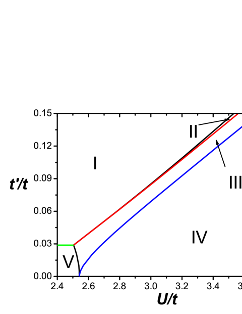
Figure 1: (Color online) The phase diagram for the case of $\varepsilon=0.15$ : I is QAH state, II is A-TSDW, III is B-TSDW, IV is trivial SDW, V is NI. The black, red and blue lines are the critical lines of $(U/t)_{M}$, $(U/t)_{c1}$ and $(U/t)_{c2},$ respectively.

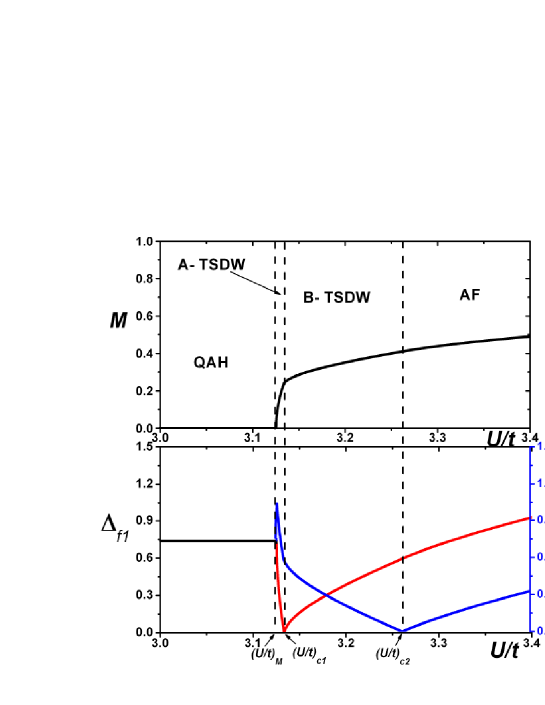
Figure 2: (Color online) The staggered magnetization and the energy gaps $\Delta_{f1}$, $\Delta_{f2}$ for the fermion excitations at node $\mathbf{k}_{1}$, $\mathbf{k}_{2}$ for the case of $\varepsilon=0.15$ and $t^{\prime}=0.1$. Below $(U/t)_{M}$, $\Delta_{f1}=\Delta_{f2}$, that is the black line; above $(U/t)_{M}$, the red line denotes $\Delta_{f1}$ and the blue line denotes $\Delta_{f2}$.

Based on the MF results, the TKNN numbers in A-TSDW, B-TSDW and the trivial SDW states are $\mathcal{Q}=2$, $\mathcal{Q}=1$, $\mathcal{Q}=0$, respectively. However, due to the quantum spin fluctuations, the classification of SDW states by the TKNN number is insufficient to give the final answer. Instead, a 2-by-2 matrix ($\mathcal{K}$-matrix) plays a key role in the topological classification of the SDW orders with the same local order parameter, $M$.

Induced CSH terms and $K$-matrices representation of TSDWs: In this part we will derive the low energy effective theory of (T-)SDW states by considering quantum fluctuations of effective spin moments based on a formulation by keeping spin rotation symmetry, $\sigma_{z}\rightarrow\mathbf{n}\cdot\mathbf{\sigma}$ where $\mathbf{n}$ is the SDW order parameter, $\left\langle\hat{c}_{i}^{\dagger}\mathbf{\sigma}\hat{c}_{i}\right\rangle=M\mathbf{n}$. In this case, the Dirac-like effective Lagrangian with spin rotation symmetry in the continuum limit can be obtained as

$$\mathcal{L}_{f}=\sum_{a}\left[i\bar{\psi}_{a}\gamma_{\mu}\left(\partial_{\mu}-iA_{\mu}\right)\psi_{a}+m_{a}\bar{\psi}_{a}\psi_{a}-\delta\Delta_{M}\bar{\psi}_{a}\mathbf{\sigma}\cdot\mathbf{n}\psi_{a}\right]$$ (3)

which describes low energy charged fermionic modes $a=1$ near $\mathbf{k}_{1},$ $\bar{\psi}_{1}=\psi_{1}^{\dagger}\gamma_{0}=(\begin{array}[]{llll}\bar{\psi}_{\uparrow 1A},&\bar{\psi}_{\uparrow 1B},&\bar{\psi}_{\downarrow 1A},&\bar{\psi}_{\downarrow 1B}\end{array})$ and $a=2$ near $\mathbf{k}_{2}$, $\bar{\psi}_{2}=\psi_{2}^{\dagger}\gamma_{0}=(\begin{array}[]{llll}\bar{\psi}_{\uparrow 2B},&\bar{\psi}_{\uparrow 2A},&\bar{\psi}_{\downarrow 2B},&\bar{\psi}_{\downarrow 2A}\end{array}).$ The masses of two-flavor fermions are $m_{1}=\varepsilon-3\sqrt{3}t^{\prime}$ and $m_{2}=\varepsilon+3\sqrt{3}t^{\prime}$. $\gamma_{\mu}$ is defined as $\gamma_{0}=\sigma_{0}\otimes\tau_{z},$ $\gamma_{1}=\sigma_{0}\otimes\tau_{y},$ $\gamma_{2}=\sigma_{0}\otimes\tau_{x}$ with $\sigma_{0}=\left(\begin{array}[]{ll}1&0\\ 0&1\end{array}\right)$. $\tau_{x},$ $\tau_{y},$ $\tau_{z}$ are Pauli matrices. $\delta$ $=$ $1$ for $a=1$ and $\delta=-1$ for $a=2$. We have set the Fermi velocity to be unit $v_{F}=1$.

In CP¹ representation, we may rewrite the effective Lagrangian of fermions in Eq.(3) as

$$\mathcal{L}_{f}=\sum_{a}\bar{\psi}_{a}^{\prime}\left(i\gamma_{\mu}\partial_{\mu}+\gamma_{\mu}A_{\mu}-\gamma_{\mu}\sigma_{3}a_{\mu}+m_{a}-\delta\Delta_{M}\sigma_{3}\right)\psi_{a}^{\prime}$$ (4)

with $\psi_{a}^{{}^{\prime}}\left(r,\tau\right)=U^{\dagger}\left(r,\tau\right)\psi_{a}\left(r,\tau\right)$, where $U\left(r,\tau\right)$ is a local and time-dependent spin SU(2) transformation defined by $U^{\dagger}\left(r,\tau\right)\mathbf{n\cdot\sigma}U\left(r,\tau\right)=\sigma_{3}$. And $a_{\mu}$ is introduced as an assistant gauge field as $i\sigma_{3}a_{\mu}\equiv U^{\dagger}\left(r,\tau\right)\partial_{\mu}U\left(r,\tau\right).$

An important property of above model in Eq.(4) is the current anomaly. The vacuum expectation value of the fermionic current $J_{a,\sigma}^{\mu}=i\langle\bar{\psi}_{a,\sigma}\gamma^{\mu}\psi_{a,\sigma}\rangle$ can be defined by $J_{a,\sigma}^{\mu}=i\{\gamma^{\mu}[(i\hat{D}+im_{a,\sigma}\mathbf{)}^{\dagger}(i\hat{D}+im_{a,\sigma}\mathbf{)}]^{-1}(i\hat{D}+im_{a,\sigma}\mathbf{)}^{\dagger}\}$ where $\hat{D}=\gamma_{\mu}(\partial_{\mu}-iA_{\mu}+i\sigma a_{\mu})$ and the mass terms are $m_{a,\sigma}=m_{a}-\delta\Delta_{M}\sigma$. The topological current $J_{a,\sigma}^{\mu}$ is obtained to be

$$J_{a,\sigma}^{\mu}=\frac{1}{2}\frac{1}{4\pi}\frac{m_{a,\sigma}}{|m_{a,\sigma}|}\epsilon^{\mu\nu\lambda}(\partial_{\nu}A_{\lambda}-\sigma\partial_{\nu}a_{\lambda}).$$ (5)

Then we derive the CSH terms as $\mathcal{L}_{CSH}=-i\sum_{a,\sigma}(A_{\mu}-\sigma a_{\mu})J_{a,\sigma}^{\mu}$redlich ; cs .

To make an explicit description of TSDWs, we introduce the $\mathcal{K}$-matrix formulation that has been used to characterize FQH fluids successfullyKmat . Now the CSH term is written as

$$\mathcal{L}_{CSH}=-i\sum_{I,J}\frac{\mathcal{K}_{IJ}}{4\pi}\varepsilon^{\mu\nu\lambda}a_{\mu}^{I}\partial_{\nu}a_{\lambda}^{J}$$ (6)

where $\mathcal{K}$ is 2-by-2 matrix, $a_{\mu}^{I=1}=A_{\mu}$ and $a_{\mu}^{I=2}=a_{\mu}.$ The ”charge” of $A_{\mu}$ and $a_{\mu}$ are defined by $q$ and $q_{s}$, respectively.

Thus for different SDW orders with the same order parameter $M$, we have different $\mathcal{K}$-matrices : for A-TSDW order with $m_{1},$ $m_{2}>\Delta_{M},$ $\mathcal{K}=\left(\begin{array}[]{ll}2&0\\ 0&2\end{array}\right);$ for B -TSDW order with $m_{2}>\Delta_{M}>m_{1}$, $\mathcal{K}=\left(\begin{array}[]{ll}1&1\\ 1&1\end{array}\right);$ for trivial SDW order with $m_{1},$ $m_{2}<\Delta_{M}$, $\mathcal{K}=0.$ It is obvious that such topological structure labeled by $\mathcal{K}$-matrices is beyond Landau’s symmetry breaking paradigm and TKNN number classification.

In the following parts we will use the following effective model with the CSH term to learn the topological properties of different SDW orders, $\mathcal{L}_{\mathrm{eff}}=\mathcal{L}_{f}+\mathcal{L}_{CSH}$.

A-TSDW: In A-TSDW, an important property is ”spin-charge separated charge-flux binding” effect for gauge fields $a_{\lambda}$ and $A_{\lambda}$. From the effective CSH Lagrangian in Eq.(6), we get the equations of motion for $a_{\lambda}$ and $A_{\lambda},$

$$\frac{1}{\pi}\epsilon^{\mu\nu\lambda}\partial_{\nu}A_{\lambda}=-J_{\mu},\text{ }\frac{1}{\pi}\epsilon^{\mu\nu\lambda}\partial_{\nu}a_{\lambda}=-J_{s\mu}$$ (7)

where $J_{\mu}=i\langle\sum_{a}\bar{\psi}_{a}\gamma_{\mu}\psi_{a}\rangle$ and $J_{s\mu}=-i\langle\sum_{a}\bar{\psi}_{a}^{\prime}\gamma_{\mu}\sigma_{3}\psi_{a}^{\prime}\rangle=-i\langle\sum_{a}\bar{\psi}_{a}\gamma_{\mu}\mathbf{n\cdot\sigma}\psi_{a}\rangle.$ As a result, we get the identities $\Phi^{e}/\pi=-q$ and $\Phi^{s}/\pi=-q_{s}$.

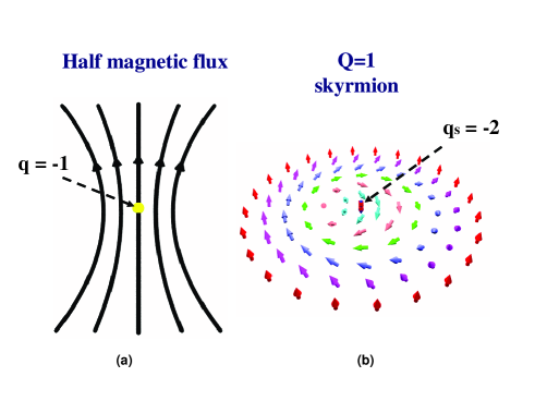
Figure 3: (Color online) Spin-charge separated charge-flux binding effect of A-TSDW : the induced quantum numbers on a half magnetic flux (a) and those on a $Q=1$ skyrmion (b).

On the one hand, the unit magnetic flux of $A_{\lambda}$, $\Phi^{e}=\int d^{2}\mathbf{r}\epsilon^{0\nu\lambda}\partial_{\nu}A_{\lambda}$, will bind electric charge $q=-2$. For example, a half magnetic flux $\Phi^{e}=\pi$ will carry $q=-1$ electric charge at its core (see FIG.3.(a)). On the other hand, the unit ”magnetic flux” of $a_{\lambda}$ will bind ”charge” $q_{s}=-2$ (see FIG.3.(b)). The ”magnetic flux” of $a_{\mu}$ is in fact the topological spin texture of SDW order (so called $Q$ skyrmion) that is characterized by winding number $Q=\frac{1}{4\pi}\int\mathbf{d^{2}\mathbf{r}}\epsilon_{0\nu\lambda}\mathbf{n\cdot\partial_{\nu}\mathbf{n}\times\partial_{\lambda}\mathbf{n}}$pol from the relation $\partial_{\nu}a_{\lambda}-\partial_{\lambda}a_{\nu}=\frac{1}{2}\mathbf{n}\cdot\partial_{\nu}\mathbf{n}\times\partial_{\lambda}\mathbf{n}$. Thus in A-TSDW, each skyrmion with $\Phi^{s}=2\pi Q$ ”magnetic flux” will accompany by additional ”charge” number $q_{s}=-2Q$. As a result, skyrmion’s spin is $S=Q^{2}\Theta/2\pi$ with $\Theta=2\pi.$ For example, by binding $q_{s}=-2$ ”charge”, the spin of $Q=1$ skyrmion is $S=1$.

Furthermore, if there exists a tiny easy-plane anisotropic term (for example, the spin-orbital coupling term), we can define the skyrmion with fractional winding number - the half skyrmion with $Q=\pm 1/2$, of which the induced ”charge” is $q_{s}=\mp 1$. However, because the energy of the half skyrmion in a long range SDW order diverges logarithmically, we cannot treat it as a real quasiparticle.

In A-TSDW, from the CS term $-\frac{i}{2\pi}\epsilon^{\mu\nu\lambda}A_{\mu}\partial_{\nu}A_{\lambda}$ and Hopf term $-\frac{i}{2\pi}\epsilon^{\mu\nu\lambda}a_{\mu}\partial_{\nu}a_{\lambda}$, we find four right-moving branches of edge excitations instead of two, which are described by the following one dimension (1D) fermion theory

$$\mathcal{L}_{\text{{edge}}}=\sum_{\alpha}\psi_{c,\alpha}^{{\dagger}}(\partial_{t}-v_{c}\partial_{x})\psi_{c,\alpha}+\sum_{\beta}\psi_{s,\beta}^{{\dagger}}(\partial_{t}-v_{s}\partial_{x})\psi_{s,\beta},$$ (8)

where $\alpha,\beta=1,2.$ $\psi_{c,\alpha}$ carries a unit of $A_{\mu}$ charge and $\psi_{s,\beta}$ a unit of $a_{\mu}$ charge7 . That means we get spin-charge separated edge states : two edge modes only carry electric charge current; two only carry spin current.

Consequently, we can define two types of Hall conductivities : the quantized charge Hall conductivity $\sigma_{H}=\lim_{\omega\rightarrow 0}{\frac{1}{\omega}}\epsilon_{ij}\left\langle J_{i}(\omega,0)J_{j}(-\omega,0)\right\rangle$ and the quantized spin Hall conductivity $\sigma_{s}=\lim_{\omega\rightarrow 0}{\frac{1}{\omega}}\epsilon_{ij}\left\langle J_{si}(\omega,0)J_{sj}(-\omega,0)\right\rangle.$ Here $J_{i}$ denotes electric current, $J_{i}=i\langle\sum_{a}\bar{\psi}_{a}\gamma_{i}\psi_{a}\rangle,$ and $J_{si}$ denotes spin current, $J_{si}=-i\langle\sum_{a}\bar{\psi}_{a}\gamma_{i}\mathbf{n\cdot\sigma}\psi_{a}\rangle$. From the CSH term, we obtain quantized Hall conductivities : $\sigma_{H}=\sigma_{s}=2e^{2}/h$ that correspond to the spin-charge separated edge statesnote1 .

B-TSDW: In B-TSDW, the equations of motion for $a_{\mu}$ and $A_{\mu}$ turn into

$$\frac{1}{2\pi}\epsilon^{\mu\nu\lambda}\partial_{\nu}A_{\lambda}+\frac{1}{2\pi}\epsilon^{\mu\nu\lambda}\partial_{\nu}a_{\lambda}=-J_{\mu}$$ (9)

and

$$\frac{1}{2\pi}\epsilon^{\mu\nu\lambda}\partial_{\nu}A_{\lambda}+\frac{1}{2\pi}\epsilon^{\mu\nu\lambda}\partial_{\nu}a_{\lambda}=-J_{s\mu}.$$ (10)

As a result, in B-TSDW, due to ”spin-charge synchronized charge-flux binding” effect from the identities $\Phi^{s}/2\pi+\Phi^{e}/2\pi=-q=-q_{s}$, the induced electric charge number is always equal to the induced ”charge” number of $a_{\mu}$ on a topological object.

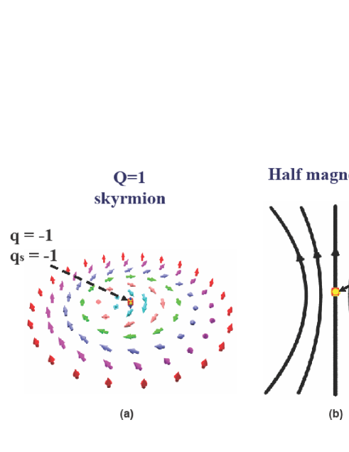
Figure 4: (Color online) Spin-charge synchronized charge-flux binding effect of B-TSDW : the induced quantum numbers on a $Q=1$ skyrmion (a) and those on a half magnetic flux (b).

On the one hand, due to the condition $\Phi^{s}/2\pi=-q=-q_{s},$ $Q$ skyrmion will carry $q=-Q$ electric charge of gauge field $A_{\mu}$ and $q_{s}=-Q$ ”charge” of gauge field $a_{\mu}$. For example, $Q=1$ skyrmion carries a unit electric charge $q=-1$ and a unit ”charge” $q_{s}=-1$ (see FIG.4.(a)). With a unit ”charge” $q_{s}$, $Q=1$ skyrmion gets half spin and becomes a charged $S=1/2$ fermion; For a $Q=2$ skyrmion, there exist two induced charge numbers on it, $q=-2,$ $q_{s}=-2$. Then it becomes a charged $S=2$ boson. In addition, for a SDW order with easy-plane anisotropic energy, we have the half skyrmion with fractional winding number $Q=\pm 1/2$, of which there exist fractional charge numbers, $q=\mp 1/2,$ $q_{s}=\mp 1/2.$ On the other hand, using the same approach, from $\Phi^{e}/2\pi=-q=-q_{s},$ we find that a half quantized magnetic flux $\Phi^{e}=\pi$ will also carry fractional charge numbers, $q=-1/2,$ $q_{s}=-1/2$ (see FIG.4.(b)).

For B-TSDW, due to a mutual CS term, $-\frac{i}{2\pi}\epsilon^{\mu\nu\lambda}A_{\mu}\partial_{\nu}a_{\lambda},$ there is no spin-charge separated edge states. Instead, we have spin-charge synchronized edge states. Now the charge of $a_{+,\mu}=A_{\mu}+a_{\mu}$ is quantized to an integer number. Then the effective CSH field theory has one right-moving edge excitation. The edge excitation is described by the following 1D fermion theory $\mathcal{L}_{\text{{edge}}}=\tilde{\psi}^{{\dagger}}(\partial_{t}-\tilde{v}\partial_{x})\tilde{\psi}$ where $\tilde{\psi}$ carries a unit of $a_{+,\mu}$ ”charge”7 . Then we may define the spin-charge synchronized Hall conductivity as $\tilde{\sigma}=\lim_{\omega\rightarrow 0}{\frac{1}{\omega}}\epsilon_{ij}\left\langle\tilde{J}_{i}(\omega,0)\tilde{J}_{j}(-\omega,0)\right\rangle$ with $\tilde{J}_{i}=i\langle\sum_{a}\bar{\psi}_{a,\downarrow}^{\prime}\gamma_{i}\psi_{a,\downarrow}^{\prime}\rangle=i\langle\sum_{a}\bar{\psi}_{a}\gamma_{i}(1-\mathbf{n\cdot\sigma)}\psi_{a}/2\rangle$ and get a quantized spin-charge synchronized Hall conductivity : $\tilde{\sigma}=\frac{e^{2}}{h}$ that corresponds to the edge state. That means an electric field can drive both a quantized electric charge current and a quantized spin current. In particular, such a quantized spin-charge synchronized Hall effect is not QAH effect for electrons with confined spin-charge degrees of freedom in QAH state.

Conclusion: In this paper, we investigate the topological Hubbard model on honeycomb lattice. New types of quantum states - A-TSDW and B-TSDW states are explored which bear an identical staggered magnetization $M$ as the local order parameter. To characterize different TSDWs, we introduce $\mathcal{K}$-matrices to denote different CSH gauge theories. In the formulism of the CSH gauge field theories with different $\mathcal{K}$-matrices, we found spin-charge separated charge-flux binding effect in A-TSDW and spin-charge synchronized charge-flux binding effect in B-TSDW. In addition we studies the edge states and corresponding quantized Hall effect in TSDWs. Our findings suggest that although there exists spontaneous spin rotation symmetry breaking, the TSDWs are beyond Landau’s paradigm.

.1 The detailed calculations of the Chern-Simons-Hopf (CSH) terms in Eq.(6)

Firstly we calculate the induced Chern-Simons (CS) term of a one flavor fermionic-$\sigma$ model. The Lagrangian of one flavor fermionic-$\sigma$ model is written as

$$\mathcal{L}=i\bar{\psi}\gamma_{\mu}(\partial_{\mu}-ib_{\mu})\psi+m\bar{\psi}\psi$$

where $m$ is a fermion mass. To obtain the induced CS term, we integrating over fermions and get

$$S_{\mathrm{eff}}=\ln\mathcal{Z}$$

where

$$\mathcal{Z}=\int[d\psi][d\bar{\psi}]\exp{(-\int dx\mathcal{L}})\mathbf{.}$$

The one fermion loop effective action becomes

$$S_{\mathrm{eff}} =\ln\det(i\gamma_{\mu}\partial_{\mu}+\gamma_{\mu}b_{\mu}+m)$$ (11)

$$=\,\mathrm{tr}\log(i\gamma_{\mu}\partial_{\mu}+m)+\mathrm{tr}({\frac{1}{i\gamma_{\mu}\partial_{\mu}+m}}\gamma_{\mu}b_{\mu})$$

$$+\frac{1}{2}\,\mathrm{tr(}{\frac{1}{i\gamma_{\mu}\partial_{\mu}+m}}\cdot\gamma_{\mu}b_{\mu}{\frac{1}{i\gamma_{\mu}\partial_{\mu}+m}}\gamma_{\mu}b_{\mu})+\dots$$

Then the quadratic term of $b_{\mu}$ in the effective action is

$$S_{\mathrm{eff}}=\frac{1}{2}\int{\frac{d^{3}p}{(2\pi)^{3}}}\left[b^{\mu}(-p)D^{\mu\nu}b^{\nu}(p)\right]$$ (12)

where $D^{\mu\nu}$ is

$$D^{\mu\nu}=\int{\frac{d^{3}k}{(2\pi)^{3}}}\,\mathrm{tr}\left[\gamma^{\mu}\,{\frac{p_{\mu}\gamma_{\mu}+k_{\mu}\gamma_{\mu}-m}{(p+k)^{2}+m^{2}}}\,\gamma^{\nu}\,{\frac{k_{\mu}\gamma_{\mu}-m}{k^{2}+m^{2}}}\right].$$ (13)

Under $\mathrm{tr}(\gamma^{\mu}\gamma^{\nu}\gamma^{\lambda})=-2\epsilon^{\mu\nu\lambda},$ we obtain

$$D^{\mu\nu}(p,m) =\epsilon^{\mu\nu\lambda}p_{\lambda}2m\int{\frac{d^{3}k}{(2\pi)^{3}}}{\frac{1}{[(p+k)^{2}+m^{2}][k^{2}+m^{2}]}}$$ (14)

$$=\epsilon^{\mu\nu\lambda}p_{\lambda}\frac{1}{2\pi}\frac{m}{|p|}\arcsin({\frac{|p|}{\sqrt{p^{2}+4m^{2}}}}).$$

In the long wavelength limit, ($\frac{p}{m}\rightarrow 0$), due to $\Theta\sim\,\frac{1}{4\pi}\frac{m}{|m|}$, we get an induced CS term as

$$\mathcal{L}_{\mathrm{eff}}=-\frac{i}{8\pi}\frac{m}{|m|}\epsilon^{\mu\nu\lambda}b_{\mu}\partial_{\nu}b_{\lambda}$$ (15)

Next we calculate the induced CSH term in Eq.(6) in the paper that denotes a four-component fermionic model

$$\mathcal{L}_{1\uparrow}=\bar{\psi}_{1\uparrow}^{\prime}\left(i\gamma^{\mu}\partial_{\mu}+\gamma^{\mu}A_{\mu}-\gamma^{\mu}a_{\mu}+m_{1}-\Delta_{M}\right)\psi_{1\uparrow}^{\prime}.$$

$$\mathcal{L}_{1\downarrow}=\bar{\psi}_{1\downarrow}^{\prime}\left(i\gamma^{\mu}\partial_{\mu}+\gamma^{\mu}A_{\mu}+\gamma^{\mu}a_{\mu}+m_{1}+\Delta_{M}\right)\psi_{1\downarrow}^{\prime}.$$

$$\mathcal{L}_{2\uparrow}=\bar{\psi}_{2\uparrow}^{\prime}\left(i\gamma^{\mu}\partial_{\mu}+\gamma^{\mu}A_{\mu}-\gamma^{\mu}a_{\mu}+m_{2}+\Delta_{M}\right)\psi_{2\uparrow}^{\prime}.$$

$$\mathcal{L}_{2\downarrow}=\bar{\psi}_{2\downarrow}^{\prime}\left(i\gamma^{\mu}\partial_{\mu}+\gamma^{\mu}A_{\mu}+\gamma^{\mu}a_{\mu}+m_{2}-\Delta_{M}\right)\psi_{2\downarrow}^{\prime}.$$

Integrating $\psi_{1\uparrow}^{\prime},$ we get the induced CS term

$$\mathcal{L}_{1\uparrow}(A_{\mu})=-\frac{i}{8\pi}\frac{m_{1}-\Delta_{M}}{|m_{1}-\Delta_{M}|}\epsilon^{\mu\nu\lambda}(A_{\mu}-a_{\mu})\partial_{\nu}(A_{\lambda}-a_{\lambda});$$

Integrating $\psi_{1\downarrow}^{\prime},$ we get the induced CS term

$$\mathcal{L}_{1\downarrow}(A_{\mu})=-\frac{i}{8\pi}\frac{m_{1}+\Delta_{M}}{|m_{1}+\Delta_{M}|}\epsilon^{\mu\nu\lambda}(A_{\mu}+a_{\mu})\partial_{\nu}(A_{\lambda}+a_{\lambda});$$

Integrating $\psi_{2\uparrow}^{\prime},$ we get the induced CS term

$$\mathcal{L}_{2\uparrow}(A_{\mu})=-\frac{i}{8\pi}\frac{m_{2}+\Delta_{M}}{|m_{2}+\Delta_{M}|}\epsilon^{\mu\nu\lambda}(A_{\mu}-a_{\mu})\partial_{\nu}(A_{\lambda}-a_{\lambda});$$

Integrating $\psi_{2\downarrow}^{\prime},$ we get the induced CS term

$$\mathcal{L}_{2\downarrow}(A_{\mu})=-\frac{i}{8\pi}\frac{m_{2}-\Delta_{M}}{|m_{2}-\Delta_{M}|}\epsilon^{\mu\nu\lambda}(A_{\mu}+a_{\mu})\partial_{\nu}(A_{\lambda}+a_{\lambda}).$$

Then we get the total induced CSH term as

$$\mathcal{L}(A_{\mu})=\mathcal{L}_{1\uparrow}(A_{\mu})+\mathcal{L}_{1\downarrow}(A_{\mu})+\mathcal{L}_{2\uparrow}(A_{\mu})+\mathcal{L}_{2\downarrow}(A_{\mu}).$$

(i) For the case of $m_{1},$ $m_{2}>\Delta_{M},$ we get

$$\mathcal{L}(A_{\mu}) =\mathcal{L}_{1\uparrow}(A_{\mu})+\mathcal{L}_{1\downarrow}(A_{\mu})+\mathcal{L}_{2\uparrow}(A_{\mu})+\mathcal{L}_{2\downarrow}(A_{\mu})$$

$$=-\frac{i}{8\pi}\epsilon^{\mu\nu\lambda}(A_{\mu}+a_{\mu})\partial_{\nu}(A_{\lambda}+a_{\lambda})$$

$$-\frac{i}{8\pi}\epsilon^{\mu\nu\lambda}(A_{\mu}-a_{\mu})\partial_{\nu}(A_{\lambda}-a_{\lambda})$$

$$-\frac{i}{8\pi}\epsilon^{\mu\nu\lambda}(A_{\mu}-a_{\mu})\partial_{\nu}(A_{\lambda}-a_{\lambda})$$

$$-\frac{i}{8\pi}\epsilon^{\mu\nu\lambda}(A_{\mu}+a_{\mu})\partial_{\nu}(A_{\lambda}+a_{\lambda})$$

$$=\frac{-i}{2\pi}\epsilon^{\mu\nu\lambda}A_{\mu}\partial_{\nu}A_{\lambda}+\frac{-i}{2\pi}\epsilon^{\mu\nu\lambda}a_{\mu}\partial_{\nu}a_{\lambda};$$

(ii) For the case of $m_{2}>\Delta_{M}>m_{1},$ we get

$$\mathcal{L}(A_{\mu}) =\mathcal{L}_{1\uparrow}(A_{\mu})+\mathcal{L}_{1\downarrow}(A_{\mu})+\mathcal{L}_{2\uparrow}(A_{\mu})+\mathcal{L}_{2\downarrow}(A_{\mu})$$

$$=-\frac{i}{8\pi}\epsilon^{\mu\nu\lambda}(A_{\mu}+a_{\mu})\partial_{\nu}(A_{\lambda}+a_{\lambda})$$

$$+\frac{i}{8\pi}\epsilon^{\mu\nu\lambda}(A_{\mu}-a_{\mu})\partial_{\nu}(A_{\lambda}-a_{\lambda})$$

$$-\frac{i}{8\pi}\epsilon^{\mu\nu\lambda}(A_{\mu}-a_{\mu})\partial_{\nu}(A_{\lambda}-a_{\lambda})$$

$$-\frac{i}{8\pi}\epsilon^{\mu\nu\lambda}(A_{\mu}+a_{\mu})\partial_{\nu}(A_{\lambda}+a_{\lambda})$$

$$=\frac{-i}{4\pi}\epsilon^{\mu\nu\lambda}A_{\mu}\partial_{\nu}A_{\lambda}+\frac{-i}{2\pi}\epsilon^{\mu\nu\lambda}A_{\mu}\partial_{\nu}a_{\lambda}+\frac{-i}{4\pi}\epsilon^{\mu\nu\lambda}a_{\mu}\partial_{\nu}a_{\lambda};$$

(iii) For the case of $m_{1},$ $m_{2}<\Delta_{M},$ we get

$$\mathcal{L}(A_{\mu}) =\mathcal{L}_{1\uparrow}(A_{\mu})+\mathcal{L}_{1\downarrow}(A_{\mu})+\mathcal{L}_{2\uparrow}(A_{\mu})+\mathcal{L}_{2\downarrow}(A_{\mu})$$

$$=-\frac{i}{8\pi}\epsilon^{\mu\nu\lambda}(A_{\mu}+a_{\mu})\partial_{\nu}(A_{\lambda}+a_{\lambda})$$

$$+\frac{i}{8\pi}\epsilon^{\mu\nu\lambda}(A_{\mu}-a_{\mu})\partial_{\nu}(A_{\lambda}-a_{\lambda})$$

$$-\frac{i}{8\pi}\epsilon^{\mu\nu\lambda}(A_{\mu}-a_{\mu})\partial_{\nu}(A_{\lambda}-a_{\lambda})$$

$$+\frac{i}{8\pi}\epsilon^{\mu\nu\lambda}(A_{\mu}+a_{\mu})\partial_{\nu}(A_{\lambda}+a_{\lambda})$$

$$=0.$$

Finally, by the $\mathcal{K}$-matrix, the CSH term is written as

$$\mathcal{L}_{CSH}=-i\sum_{I,J}\frac{\mathcal{K}_{IJ}}{4\pi}\varepsilon^{\mu\nu\lambda}a_{\mu}^{I}\partial_{\nu}a_{\lambda}^{J}$$ (16)

where $\mathcal{K}$ is 2-by-2 matrix, $a_{\mu}^{I=1}=A_{\mu}$ and $a_{\mu}^{I=2}=a_{\mu}.$ Thus for different SDW orders with the same order parameter $M$, we have different $\mathcal{K}$-matrices : for $m_{1},$ $m_{2}>\Delta_{M},$ $\mathcal{K}=\left(\begin{array}[]{ll}2&0\\ 0&2\end{array}\right);$ for $m_{2}>\Delta_{M}>m_{1}$, $\mathcal{K}=\left(\begin{array}[]{ll}1&1\\ 1&1\end{array}\right);$ for $m_{1},$ $m_{2}<\Delta_{M}$, $\mathcal{K}=0.$

References

• (1) K. V. Klitzing, et al., Phys. Rev. Lett. 45, 494 (1980).
• (2) D. J. Thouless, et al., Phys. Rev. Lett. 49, 405 (1982).
• (3) D. C. Tsui, et al., Phys. Rev. Lett. 48, 1559 (1982).
• (4) R. B. Laughlin, Phys. Rev .Lett. 50, 1395 (1983).
• (5) X.-G. Wen, Phys. Rev. B 40, 7387 1989. X.-G. Wen, Int. J. Mod. Phys. B 4, 239 1990.
• (6) X.-G. Wen, Quantum Field Theory of Many-Body Systems, (Oxford University Press, 2004).
• (7) C. L. Kane and E. J. Mele, Phys. Rev. Lett.  95, 146802 (2005); 95, 226801 (2005).
• (8) B. A. Bernevig and S.-C. Zhang, Phys. Rev. Lett. 96, 106802 (2006).
• (9) B. Blok and X.-G. Wen, Phys. Rev. B 42 8133 (1990).
• (10) To define a quantized spin Hall conductivity, we need to add an additional easy-axis anisotropic energy term to open a small spin gap.
• (11) A. A. Belavin and A. M. Polyakov, JETP Lett. 22, 245 (1975).
• (12) F. D. M. Haldane, Phys. Rev. Lett. 61, 2015 (1988).
• (13) J. He, et al., arXiv: 1012.0620, accepted by PHYS. REV. B.
• (14) A. N. Redlich, Phys. Rev. Lett. 52 (1984) 18, Phys. Rev. D 29 (1984) 2366.
• (15) K. Ishikawa and T. Matsuyama, Z. Phys. C 33, 41 (1986); Nucl. Phys. B 280, 523 (1987).