Root’s barrier: Construction, optimality and applications to variance options

Abstract

Recent work of Dupire and Carr and Lee has highlighted the importance of understanding the Skorokhod embedding originally proposed by Root for the model-independent hedging of variance options. Root’s work shows that there exists a barrier from which one may define a stopping time which solves the Skorokhod embedding problem. This construction has the remarkable property, proved by Rost, that it minimizes the variance of the stopping time among all solutions.

In this work, we prove a characterization of Root’s barrier in terms of the solution to a variational inequality, and we give an alternative proof of the optimality property which has an important consequence for the construction of subhedging strategies in the financial context.

and

1 Introduction

In this paper, we analyze the solution to the Skorokhod embedding problem originally given by Root Root69 , and generalized by Rost Rost76 . Our motivation for this is recent work connecting the solution to this problem to questions arising in mathematical finance—specifically model-independent bounds for variance options—which has been observed by Dupire dupire , Carr and Lee CarrLee10 and Hobson HobsonSurvey . The financial motivation can be described as follows: consider a (discounted) asset which has dynamics under the risk-neutral measure

$$\frac{\mathrm{d}S_{t}}{S_{t}}=\sigma_{t}\,\mathrm{d}W_{t},$$

where the process $\sigma_{t}$ is not necessarily known. We are interested in variance options, which are contracts where the payoff depends on the realized quadratic variation of the log-price process: specifically, we have

$$\mathrm{d}(\ln S_{t})=\sigma_{t}\,\mathrm{d}W_{t}-\tfrac{1}{2}\sigma_{t}^{2}\,\mathrm{d}t$$

and therefore

$$\langle\ln S\rangle_{T}=\int_{0}^{T}\sigma_{t}^{2}\,\mathrm{d}t.$$

An option on variance is then an option with payoff $F(\langle\ln S\rangle_{T})$. Important examples include variance swaps, which pay the holder $\langle\ln S\rangle_{T}-K$, and variance calls which pay the holder $(\langle\ln S\rangle_{T}-K)_{+}$. We shall be particularly interested in the case of a variance call, but our results will extend to a wider class of payoffs. Let $\mathrm{d}X_{t}=X_{t}\,\mathrm{d}\widetilde{W}_{t}$ for a suitable Brownian motion $\widetilde{W}_{t}$ and we can find a (continuous) time change $\tau_{t}$ such that $S_{t}=\widetilde{X}_{\tau_{t}}$, and so

$$\mathrm{d}\tau_{t}=\frac{\sigma_{t}^{2}S_{t}^{2}}{S_{t}^{2}}\,\mathrm{d}t.$$

Hence

$$(\widetilde{X}_{\tau_{T}},\tau_{T})=\biggl{(}S_{T},\int_{0}^{T}\sigma_{u}^{2}\,\mathrm{d}u\biggr{)}=(S_{T},\langle\ln S\rangle_{T}).$$

Now suppose that we know the prices of call options on $S_{T}$ with maturity $T$, and at all strikes (recall that $\sigma_{t}$ is not assumed known). Then we can derive the law of $S_{T}$ under the risk-neutral measure from the Breeden–Litzenberger formula. Call this law $\mu$. This suggests that the problem of finding a lower bound on the price of a variance call (for an unknown $\sigma_{t}$) is equivalent to

find a stopping time $$\tau \mathbb{E}(\tau-K)_{+} \mathcal{L}(\widetilde{X}_{\tau})=\mu$$ to minimize , subject to . (1)

This is essentially the problem for which Rost has shown that the solution is given by Root’s barrier. [In fact, the result trivially extends to payoffs of the form $F(\langle\ln S\rangle_{T})$ where $F(\cdot)$ is a convex, increasing function.]

In this work, our aim is twofold: first, to provide a proof that Root’s barrier can be found as the solution to a particular variational inequality, which can be thought of as the generalization of an obstacle problem; second, we show that the lower bound which is implied by Rost’s result can be enforced through a suitable hedging strategy, which will give an arbitrage whenever the price of a variance call trades below the given lower bound. To accomplish this second part of the paper, we will give a novel proof of the optimality of Root’s construction, and from this construction we will be able to derive a suitable hedging strategy.

The use of Skorokhod embedding techniques to solve model-independent (or robust) hedging problems in finance can be traced back to Hobson Hobson98 . More recent results in this direction include Cox, Hobson and Obłój CoxHobsonObloj08 , Cox and Obłój CoxObloj11b and Cox and Obłój CoxObloj11 . For a comprehensive survey of the literature on the Skorokhod embedding problem, we refer the reader to Obłój Obloj04 . In addition, Hobson HobsonSurvey surveys the literature on the Skorokhod embedding problem with a specific emphasis on the applications in mathematical finance.

Variance options have been a topic of much interest in recent years, both from the industrial point of view, where innovations such as the VIX index have contributed to a large growth in products which are directly dependent on quantities derived from the quadratic variation, and also on the academic side, with a number of interesting contributions in the literature. The academic results go back to work of Dupire Dupire93 and Neuberger Neuberger94 , who noted that a variance swap—that is, a contract which pays $\langle\ln S\rangle_{T}$, can be replicated model-independently using a contract paying the logarithm of the asset at maturity through the identity (from Itô’s lemma)

$$\ln(S_{T})-\ln(S_{0})=\int_{0}^{T}\frac{1}{S_{t}}\,\mathrm{d}S_{t}-\frac{1}{2}\langle\ln S\rangle_{T}.$$ (2)

More recently, work on options and swaps on volatility and variance, (in a model-based setting) includes Howison, Rafailidis and Rasmussen HowisonRafailidisRasmussen04 , Broadie and Jain BroadieJain08 and Kallsen, Muhle-Karbe and Voss KallsenMuhle-KarbeVoss11 . Other work Keller-Ressel11 , Keller-ResselMuhle-Karbe10 has considered the differences between the theoretical payoff ($\langle\ln S\rangle_{T}$) and the discrete approximation which is usually specified in the contract [$\sum_{k}\ln(S_{(k+1)\delta}/S_{k\delta})^{2}$]. Finally, several papers have considered variants on the model-independent problems CarrLee10 , CarrLeeWu11 , DavisOblojRaval10 or problems where the modeling assumptions are fairly weak. This latter framework is of particular interest for options on variance, since the markets for such products are still fairly young, and so making strong modelling assumptions might not be as strongly justified as it could be in a well-established market.

The rest of this paper is structured as follows: in Section 2 we review some known results and properties concerning Root’s barrier. In Section 3, we establish a connection between Root’s solution and an obstacle problem, and then in Section 4 we show that by considering an obstacle problem in a more general analytic sense (as a variational inequality), we are able to prove the equivalence between Root’s problem and the solution to a variational inequality. In Section 5, we give a new proof of the optimality of Root’s solution and in Section 6 we show how this proof allows us to construct model-independent subhedges to give bounds on the price of variance options.

2 Features of Root’s solution

Our interest is in Root’s solution to the Skorokhod embedding problem. Simply stated, for a process $(X_{t})_{t\geq 0}$, the Skorokhod embedding problem is to find a stopping time $\tau$ such that $X_{\tau}\sim\mu$. In this paper, we will consider first the case where $X_{0}=0$, and $X_{t}$ is a continuous martingale and a time-homogeneous diffusion, and later the case where $X_{0}\sim\nu$, is a centred, square integrable measure. In such circumstances, it is natural to restrict to the set of stopping times for which $(X_{t\wedge\tau})_{t\geq 0}$ is a uniformly integrable (UI) process. We will occasionally call stopping times for which this is true UI stopping times. In the case where $\mu$ is centered and has a second moment and the underlying process $X$ is a Brownian motion (or more generally, a diffusion and martingale with diffusion coefficient $\sigma$ such that $\sigma^{2}\geq\varepsilon$ for some strictly positive constant $\varepsilon$), this is equivalent to the fact that $\mathbb{E}\tau<\infty$. For the case of a general starting measure, there is a natural restriction on the measures involved, which is that we require

$$\infty>\mathrm{U}_{\nu}(x):=-\int_{\mathbb{R}}|y-x|\nu(\mathrm{d}y)\geq-\int_{\mathbb{R}}|y-x|\mu(\mathrm{d}y)=:\mathrm{U}_{\mu}(x),$$ (3)

for all $x\in\mathbb{R}$. This assumption implies that $m:=\int x\nu(\mathrm{d}x)=\int x\mu(\mathrm{d}x)$; see Chacon MR0501374 . By Jensen’s inequality, such a constraint is clearly necessary for the existence of a suitable pair $\nu$ and $\mu$; further, by Rost Rost71 , it is the only additional constraint on the measures we will need to impose. We shall write

$$S(\mu)=\{\tau\dvtx\tau\mbox{ is a stopping time},X_{\tau}\sim\mu,(X_{t\wedge\tau})_{t\geq 0}\mbox{ is UI}\}.$$ (4)

There are a number of important papers concerning the construction of Root’s barrier. The first work to consider the problem is Root Root69 , and this paper proved the existence of a certain Skorokhod embedding when $X_{t}$ is a Brownian motion. Specifically, Root showed that if $X_{t}$ is a Brownian motion with $X_{0}=0$, and $\mu$ is the law of a centered random variable with finite variance, then there exists a stopping time $\tau$, which is the first hitting time of a barrier, which is defined as follows:

Definition 2.1 ((Root’s barrier)).

A closed subset $B$ of $[-\infty,+\infty]\times[0,+\infty]$ is a barrier if: [(1)]

$(x,+\infty)\in B$ for all $x\in[-\infty,+\infty]$;

$(\pm\infty,t)\in B$ for all $t\in[0,\infty]$;

if $(x,t)\in B$, then $(x,s)\in B$ whenever $s>t$.

We provide representative examples of barrier functions in Figure 1.

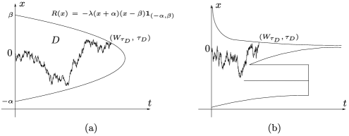
Figure 1: Examples of Root’s barriers: the representation (a) is an example of a “nice” barrier, where some explicit calculations can be made (see Example 5.6); in (b) we observe some of the nastier features which a barrier may possess, including spikes, corresponding to atoms of the distribution $\mu$ and regions in which the barrier can be unbounded.

In a subsequent paper Loynes Loynes70 proved a number of results relating to barriers. From our perspective, the most important are, first, that the barrier $B$ can be written as $B=\{(x,t)\dvtx t\geq R(x)\}$, where $R\dvtx\mathbb{R}\to[0,\infty]$ is a lower semi-continuous function (with the obvious extensions to the definition to cover $R(x)=\infty$); we will make frequent use of this representation. In addition, Loynes Loynes70 , Theorem 1, says that Root’s solution is essentially unique: if there are two barriers which embed the same distribution with a UI stopping time, then their corresponding stopping times are equal with probability one. The case where two different barriers can occur are then only the cases where, say $R(x_{0})=0$ for $x_{0}>0$, and then $R(x)$ is undetermined for all $x>x_{0}$.

The other important reference for our purposes is Rost Rost76 . This work vastly extends the generality of the results of Root and Loynes, and uses mostly potential-theoretic techniques. Rost works in the generality of a Markov process $X_{t}$ on a compact metric space $E$, which satisfies the strong Markov property and is right-continuous. Then Rost recalls (from an original definition of Dinges Dinges74 in the discrete setting) the notion of minimal residual expectation:

Definition 2.2.

A stopping time $\tau^{*}\in S(\mu)$ is of minimal residual expectation if, for each $t\in\mathbb{R}_{+}$, it minimizes the quantity

$$\mathbb{E}(\tau-t)_{+}=\mathbb{E}\int_{\tau\wedge t}^{\tau}\,\mathrm{d}s=\int_{t}^{\infty}\mathbb{P}(\tau>s)\,\mathrm{d}s,$$

over all $\tau\in S(\mu)$.

Then Rost proves that [under (3)] there exists a stopping time of minimal residual expectation Rost76 , Theorem 1, and that the hitting time of any barrier is of minimal residual expectation Rost76 , Theorem 2. Finally, Rost also shows that the barrier stopping times are, to a degree, unique Rost76 , Corollary to Theorem 2. The relevant result for our purposes (where there is a stronger form of uniqueness) is the corollary to Theorem 3 therein, which says that if $X_{t}$ is a process for which the one-point sets are regular, then any stopping time of minimal residual expectation is Root’s stopping time. The class of processes for which the one-point sets are regular include the class of time-homogenous diffusions we consider.

Note that a stopping time is of minimal residual expectation if and only if, for every convex, increasing function $F(t)$ (where, without loss of generality, we take $F(0)=F_{+}^{\prime}(0)=0$), it minimizes the quantity

$$\mathbb{E}F(\tau)=\mathbb{E}\int_{0}^{\infty}(\tau-t)_{+}F^{\prime\prime}(\,\mathrm{d}t),$$

this fact being a consequence of the above representation.

There are a number of important properties that the Root barrier possesses. First, we note that, as a consequence of the fact that $B$ is closed and the third property of Definition 2.1, the barrier is regular (i.e., if we start at a point in the barrier, we will almost surely return to the barrier instantly) for the class of processes we will consider (time-homogeneous diffusions) this will have important analytical benefits. Second, for a point $(x,t)\notin B$, we know that if the stopped process at time $t$ is at $x$, then we have not yet reached the stopping time for the embedding. This will help in our characterization of the law of the stopped process (Lemma 3.2).

In the rest of this paper, we will then say that a barrier is either a lower semi-continuous function $R\dvtx\mathbb{R}\rightarrow\overline{\mathbb{R}}_{+}$, with $R(0)\neq 0$, or the complement of the corresponding connected open set $D=\{(x,t)\dvtx 0<t<R(x)\}=\mathbb{R}\times(0,\infty)\setminus B$. As noted above, by Loynes Loynes70 this is equivalent to the barrier as defined in Definition 2.1. We will define the hitting time of the barrier as: $\tau_{D}=\inf\{t>0\dvtx(X_{t},t)\notin D\}$. Note that the barrier $B$ is closed and regular, so that $(X_{\tau_{D}},\tau_{D})\in B$ and $\mathbb{P}^{(x,t)}(\tau_{D}=0)=1$ whenever $(x,t)\in B$, where $\mathbb{P}^{(x,t)}$ is the law of our diffusion started at $x$ at time $t$.

Finally, we give some examples where the barrier function can be explicitly calculated. We note that explicit examples appear to be the exception, and in general are hard to compute. First, if $\mu$ is a Normal distribution, we easily see that $R(x)$ is a constant. Second, if $\mu$ consists of two atoms (weighted appropriately) at $a<0<b$ say, the corresponding barrier is

$$R(x)=\cases{0,&\quad$x\notin(a,b),$\vspace*{2pt}\cr\infty,&\quad$x\in(a,b).$}$$

In this example, observe that the function $R(x)$ is not unique: we can choose any behavior outside $[a,b]$, and achieve the same stopping time. Second, we note the that there are even more general solutions to the Skorokhod embedding problem (without the uniform integrability condition) since there are also barriers of the form

$$R(x)=\cases{t_{a},&\quad$x=a,$\vspace*{2pt}\cr t_{b},&\quad$x=b,$\vspace*{2pt}\cr\infty,&\quad$x\notin\{a,b\},$}$$

which will embed the same law (provided $t_{a},t_{b}>0$ are chosen suitably), but which do not satisfy the uniform integrability condition. In general, a barrier can exhibit some fairly nasty features: consider, for example, the canonical measure on a middle third Cantor set $C$ (scaled so that it is on $[-1,1]$). Root’s result tells us that there exists a barrier which embeds this distribution, and clearly the resulting barrier function must be finite only on the Cantor set; however, the target distribution has no atoms, so that the “spikes” in the barrier function can not be isolated (i.e., we must have $\liminf_{y\uparrow x}R(y)=\liminf_{y\downarrow x}R(y)=R(x)$ for all $x\in(-1,1)\cap C$).

3 Connecting Root’s problem and an obstacle problem

We now consider alternative methods for describing Root’s barrier. We will, in general, be interested in this question when our underlying process $X_{t}$ is a solution to

$$\,\mathrm{d}X_{t}=\sigma(X_{t})\,\mathrm{d}W_{t},\qquad X_{0}\sim\nu,$$ (5)

for a Brownian motion $(W_{t})_{t\geq 0}$, and we will introduce our concepts in this general context. Initially, we assume that $\sigma\dvtx\mathbb{R}\rightarrow\mathbb{R}$ satisfies, for some positive constant $K$,

$$|\sigma(x)-\sigma(y)|\leq K|x-y|;$$ (6)

$$0<\sigma^{2}(x)<K(1+x^{2});$$ (7)

$$\sigma\mbox{ is smooth.}$$ (8)

Recall that for the financial application we are interested in, we want the specific case $\sigma(x)=x$ to be included. Clearly, this case is currently excluded; however, we will show in Section 4.3 that the results can be extended to include this case.

From standard results on SDEs, (6) and (7) imply that the unique strong solution $X^{a}$ of (5) with $\nu=\delta_{a}$ is a strong Markov process with generator $\frac{1}{2}\sigma^{2}\partial_{xx}$ for any initial value $a\in\mathbb{R}$. Moreover, (8) implies that the operator $L:=\frac{1}{2}\sigma^{2}\partial_{xx}-\partial_{t}$ is hypoelliptic; see Stroock Stroock08 , Theorem 3.4.1.

We will write Root’s Skorokhod embedding problem as:

Find a lower-semicontinuous function $R(x)$ such that the domain $D=\{(x,t)\dvtx 0<t<R(x)\}$ has $X_{\tau_{D}}\sim\mu$, and $(X_{t\wedge\tau_{D}})_{t\geq 0}$ is a UI process, where $\nu$ is the initial law of $X_{t}$, and $\sigma$ the diffusion coefficient.

Our aim is to show that the problem of finding $R$ is essentially equivalent to solving an obstacle problem. Assuming that the relevant derivatives exist, we shall show that the problem can be stated in the following way:

Find a function $u(x,t)\in C^{1,1}(\mathbb{R}\times\mathbb{R}_{+})$ such that

$$\mathrm{U}_{\nu}(x)=u(x,0),$$ (9a)

$$0\geq\mathrm{U}_{\mu}(x)-u(x,t),$$ (9b)

$$\displaystyle 0\geq\frac{\partial u}{\partial t}(x,t)-\frac{1}{2}\sigma(x)^{2}\frac{\partial^{2}u}{\partial x^{2}}(x,t),$$ (9c)

$$\displaystyle\biggl{(}\frac{\partial u}{\partial t}(x,t)-\frac{1}{2}\sigma(x)^{2}\frac{\partial^{2}u}{\partial x^{2}}(x,t)\biggr{)}\bigl{(}\mathrm{U}_{\mu}(x)-u(x,t)\bigr{)}=0,$$ (9d)

where (9c) is interpreted in a distributional sense—that is, we require

$$\int_{\mathbb{R}}\biggl{(}\phi(x)\frac{\partial u}{\partial t}(x,t)+\frac{1}{2}\sigma(x)^{2}\frac{\partial u}{\partial x}(x,t)\phi^{\prime}(x)\biggr{)}\,\mathrm{d}x\leq 0$$

whenever $\phi\in C_{K}^{\infty}$ is a nonnegative function. Condition (9d) can be interpreted more generally as requiring

$$\frac{\partial u}{\partial t}(x,t)=\frac{1}{2}\sigma(x)^{2}\frac{\partial^{2}u}{\partial x^{2}}(x,t)$$

in a distributional sense whenever $(\mathrm{U}_{\mu}(x)-u(x,t))\neq 0$. However, this is an open set, and from the hypoellipticity of the operator $L$, if this holds in a weak sense, it will hold in a strong sense. Hence $\frac{\partial^{2}u}{\partial x^{2}}(x,t)$ would be continuous even if we were only to require (9d) to hold in a distributional sense.

In general, we do not expect $u$ to be sufficiently nice that we can easily interpret all these statements, and one of the goals of this paper is to give a generalization of OBS$(\sigma,\nu,\mu)$ that will make sense more widely. Cases in which $u$ may not be expected to be $C^{1,1}$ include the case where $\mu$ contains atoms (and therefore $\mathrm{U}_{\mu}$ is not continuously differentiable). In addition, we specify this problem in $C^{1,1}$ since, in general, we would certainly not expect the second derivative to be continuous on the boundary between the two types of behavior in (9d).

Theorem 3.1

Suppose $D$ is a solution to SEP$(\sigma,\nu,\mu)$ and is such that

$$u(x,t)=-\mathbb{E}|X_{t\wedge\tau_{D}}-x|\in C^{1,1}(\mathbb{R}\times\mathbb{R}_{+}).$$

Then $u$ solves OBS$(\sigma,\nu,\mu)$.

This gives an initial connection between OBS$(\sigma,\nu,\mu)$ and SEP$(\sigma,\nu,\mu)$. We roughly expect solutions to Root’s problem to be the unique solutions to the obstacle problem (of course, we do not currently know that such solutions exist or, when they do, are unique). This suggests that we can attempt to solve the obstacle problem to find the solution $D$ to Root’s problem. In particular, given a solution to OBS$(\sigma,\nu,\mu)$, we can now identify $D$ as $D=\{(x,t)\dvtx\mathrm{U}_{\mu}(x)<u(x,t),t>0\}$.

Lemma 3.2

For any $(x,t)\in D$, $\mathbb{P}(X_{t\wedge\tau_{D}}\in\mathrm{d}x)=\mathbb{P}(X_{t}\in\,\mathrm{d}x,t<\tau_{D})$.

By the lower semi-continuity of $R$, since $(x,t)\in D$, there exists $h>0$ such that

$$(x-h,x+h)\times[0,t+h)\subset D,$$

and hence, for any $y\in(x-h,x+h)$, $R(y)>t$. On the other hand, if $\tau_{D}\leq t$, we have

$$R(X_{\tau_{D}})\leq\tau_{D}\leq t,$$

and hence, $X_{\tau_{D}}\notin(x-h,x+h)$. Therefore,

$$\mathbb{P}(X_{t\wedge\tau_{D}}\in\mathrm{d}x) = \mathbb{P}(X_{t}\in\mathrm{d}x,t<\tau_{D})+\mathbb{P}(X_{\tau_{D}}\in\mathrm{d}x,t\geq\tau_{D})$$

$$= \mathbb{P}(X_{t}\in\mathrm{d}x,t<\tau_{D}).$$

Lemma 3.3

The measure corresponding to $\mathcal{L}(X_{t};t<\tau_{D})$ has density $p^{D}(x,t)$ with respect to Lebesgue on $D$, and the density is smooth and satisfies

$$\frac{\partial}{\partial t}p^{D}(x,t)=\frac{1}{2}\frac{\partial^{2}}{\partial x^{2}}[\sigma(x)^{2}p^{D}(x,t)].$$

This result appears to be standard, but we are unable to find concise references. We give a short proof based on RogersWilliamsVol2 , Section V.38.5.

Proof of Lemma 3.3 First note that, as a measure, $\mathcal{L}(X_{t};t<\tau_{D})$ is dominated by the usual transition measure, so the density $p^{D}(x,t)$ exists.

Let $(x_{0},t_{0})$ be a point in $D$, and we can therefore find an $\varepsilon>0$ such that $A=(x_{0}-\varepsilon,x_{0}+\varepsilon)\times(t_{0}-\varepsilon,t_{0}+\varepsilon)$ satisfies $\bar{A}\subseteq D$. Then let $f$ be a smooth function, supported on $A$, and by Itô’s lemma,

$$f(X_{t\wedge\tau_{D}},t) = f(X_{0},0)+\int_{0}^{t}\frac{\partial f}{\partial x}(X_{s\wedge\tau_{D}},s)\,\mathrm{d}X_{s}$$

$${}+\int_{0}^{t}\biggl{(}\frac{1}{2}\sigma(X_{s\wedge\tau_{D}})^{2}\frac{\partial^{2}}{\partial x^{2}}+\frac{\partial}{\partial t}\biggr{)}f(X_{s\wedge\tau_{D}},s)\,\mathrm{d}s.$$

Since $f$ is compactly supported, taking $t>t_{0}+\varepsilon$, the two terms on the left disappear, and the first integral term is a martingale. Hence, taking expectations, and interchanging the order of differentiation, we get

$$\int_{0}^{t}\int p^{D}(y,s)\biggl{(}\frac{1}{2}\sigma(y)^{2}\frac{\partial^{2}}{\partial x^{2}}+\frac{\partial}{\partial t}\biggr{)}f(y,s)\,\mathrm{d}y\,\mathrm{d}s=0.$$

Interpreting $p^{D}(y,s)$ as a distribution, we have

$$\frac{1}{2}\frac{\partial^{2}}{\partial x^{2}}[\sigma(x)^{2}p^{D}(x,t)]-\frac{\partial}{\partial t}p^{D}(x,t)=0,$$

for $(x,t)\in A$, and since the heat operator is hypoelliptic, we conclude that $p^{D}(x,t)$ is smooth in $A$ (e.g., Stroock Stroock08 , Theorem 3.4.1).

We are now able to prove that any solution to Root’s embedding problem is a solution to the obstacle problem.

Proof of Theorem 3.1 We first observe that $u(x,0)=-\mathbb{E}|X_{0}-x|$, and $X_{0}\sim\nu$, so that $u(x,0)=-\int|y-x|\nu(\mathrm{d}y)$ and (9a) holds. Second, since $(X_{t\wedge\tau_{D}})_{t\geq 0}$ is a UI process, by (conditional) Jensen’s inequality,

$$u(x,t)=-\mathbb{E}|x-X_{t\wedge\tau_{D}}|\geq-\mathbb{E}\bigl{[}\mathbb{E}[|x-X_{\tau_{D}}||\mathcal{F}_{t\wedge\tau_{D}}]\bigr{]}=\mathrm{U}_{\mu}(x),$$

and (9b) holds.

We now consider (9c). Suppose $(x,t)\in D$, and note that

$$\frac{\partial u}{\partial x}=1-2\mathbb{P}(X_{t\wedge\tau_{D}}<x),$$ (10)

and therefore (in $D$) by Lemma 3.3 the function $u$ has a smooth second derivative in $x$. Further, we get

$$\frac{1}{2}\int_{0}^{t}\sigma(x)^{2}\frac{\partial^{2}u}{\partial x^{2}}(x,s)\,\mathrm{d}s = -\int_{0}^{t}\sigma(x)^{2}p_{D}(x,s)\,\mathrm{d}s$$

$$= \lim_{\varepsilon\downarrow 0}\mathbb{E}\biggl{[}\frac{1}{2\varepsilon}\int_{0}^{t\wedge\tau_{D}}\sigma(x)^{2}\mathbf{1}_{[x-\varepsilon<X_{s}<x+\varepsilon]}\,\mathrm{d}s\biggr{]}$$

$$= -\mathbb{E}L_{t\wedge\tau_{D}}^{x}$$

$$= -\mathbb{E}|x-X_{t\wedge\tau_{D}}|+|x|,$$

where $L^{x}_{t}$ is the local time of the diffusion at $x$. It follows that $u$ satisfies (9c) on $D$, and in fact attains equality there. On the other hand, if $(x,t)\notin D$, it follows from the definition of the barrier that if $\tau_{D}>t$, the diffusion cannot cross the line $\{(x,s)\dvtx s\geq t\}$ in the time interval $[t,\tau_{D})$, and hence

$$L_{t\wedge\tau_{D}}^{x}=L_{t}^{x}\mathbf{1}_{\tau_{D}>t}+L_{\tau_{D}}^{x}\mathbf{1}_{\tau_{D}\leq t}=L_{\tau_{D}}^{x}\mathbf{1}_{\tau_{D}>t}+L_{\tau_{D}}^{x}\mathbf{1}_{\tau_{D}\leq t}=L_{\tau_{D}}^{x}.$$

Therefore, for $t\geq R(x)$,

$$\mathbb{E}|x-X_{t\wedge\tau_{D}}|=|x|+\mathbb{E}L^{x}_{t\wedge\tau_{D}}=|x|+\mathbb{E}L^{x}_{\tau_{D}}=\mathbb{E}|x-X_{\tau_{D}}|,$$

where the last equality holds because $\tau_{D}$ is a UI stopping time. So (9b) holds with equality when $(x,t)\notin D$. In particular, we can deduce that either (if $(x,t)\in D$) we have equality in (9c), or we have equality in (9b), in which case (9d) must hold. It remains to show that (9c) holds when $(x,t)\notin D$. However, to see this, consider $(x,t)\notin D$, and note first that $u(x,s)=u(x,t)=\mathrm{U}_{\mu}(x)$ whenever $s>t$, since $(x,s)\notin D$. Hence $\frac{\partial u}{\partial t}(x,t)=0$. It is straightforward to check that $u(x,t)$ is concave in $x$, and therefore that $\frac{\partial^{2}u}{\partial x^{2}}(x,t)\leq 0$, and (9c) also holds.

This result connects Root’s problem and the obstacle problem under a smoothness assumption on the function $u$. However, ideally we want a one-to-one correspondence. We know from the results of Rost Rost76 that there always exists a solution to SEP$(\sigma,\nu,\mu)$, and from Loynes Loynes70 that the solution is unique. Our aim is to show that a similar combination of existence and uniqueness hold for the corresponding analytic formulation. As already noted, we cannot make a strong smoothness assumption on the function $u(x,t)$ as required by OBS$(\sigma,\nu,\mu)$, and so we need a weaker formulation of this problem. Generalizations of the obstacle problem are well understood, and commonly called variational inequalities. In the next section, we will reformulate the obstacle problem as a variational inequality, and we are able to state a problem for which existence and uniqueness are known due to existing results.

4 Root’s barrier and variational inequalities

We now study the relation between Root’s Skorokhod embedding problem and a variational inequality. Our notation and definitions, and some of the key results which we will use, come from Bensoussan and Lions BensoussanLions82 .

4.1 Variational inequalities

We begin with some necessary notation and results concerning evolutionary variational inequalities. Given a constant $\lambda>0$ and a finite time $T>0$, we define the Banach spaces $H^{m,\lambda}\subseteq L^{2}(\mathbb{R})$ and $L^{2}(0,T;H^{m,\lambda})$ with the norms

$$\|g\|^{2}_{H^{m,\lambda}} = \sum_{k=0}^{m}\int_{\mathbb{R}}e^{-2\lambda|x|}\biggl{|}\frac{\partial^{k}g}{\partial x^{k}}(x)\biggr{|}^{2}\,\mathrm{d}x;$$

$$\|w\|^{2}_{L^{2}(0,T;H^{m,\lambda})} = \int_{0}^{T}\|w(\cdot,t)\|^{2}_{H^{m,\lambda}}\,\mathrm{d}t,$$

where the derivatives $\frac{\partial^{k}g}{\partial x^{k}}(x)$ are to be interpreted as weak derivatives—that is, $\frac{\partial^{k}g}{\partial x^{k}}(x)$ is defined by the requirement that

$$\int_{\mathbb{R}}\phi(x)\frac{\partial^{k}g}{\partial x^{k}}(x)\,\mathrm{d}x=(-1)^{k}\int_{\mathbb{R}}g(x)\frac{\partial^{k}\phi}{\partial x^{k}}(x)\,\mathrm{d}x,$$

for all $\phi\in C_{K}^{\infty}(\mathbb{R})$, and $C_{K}^{\infty}$ is the set of compactly supported, smooth functions on $\mathbb{R}$. In particular, the spaces $H^{m,\lambda}$ and $L^{2}(0,T;H^{m,\lambda})$ are Hilbert spaces with respect to the obvious inner products. In addition, elements of the set $H^{1,\lambda}$ can always be taken to be continuous, and $C_{K}^{\infty}$ is dense in $H^{m,\lambda}$; see, for example, Friedman FriedmanGenFunc , Theorem 5.5.20.

For functions $a(x,t),b(x,t)\in L^{\infty}(\mathbb{R}\times(0,T))$, we define an operator

$$a_{\lambda}(t;v,w)=\int_{\mathbb{R}}e^{-2\lambda|x|}\biggl{[}a(x,t)\frac{\partial v}{\partial x}\frac{\partial w}{\partial x}+b(x,t)\frac{\partial v}{\partial x}w\biggr{]}\,\mathrm{d}x,$$

for $v,w\in L^{2}(0,T;H^{1,\lambda})$. Moreover if $\partial a/\partial x$ exits, we define, for $v\in H^{2,\lambda}$,

$$A(t)v=-\frac{\partial}{\partial x}\biggl{(}a(x,t)\frac{\partial v}{\partial x}\biggr{)}+\bigl{(}b(x,t)+2\lambda a(x,t)\operatorname{sgn}(x)\bigr{)}\frac{\partial v}{\partial x}.$$

And finally, for $v,w\in H^{0,\lambda}$,

$$(v,w)_{\lambda}=\int_{\mathbb{R}}e^{-2\lambda|x|}vw\,\mathrm{d}x,$$

so that, for suitably differentiable test functions $\phi(x)$ and $v\in H^{2,\lambda}$,

$$(\phi,A(t)v)_{\lambda}=a_{\lambda}(t;v,\phi).$$

Then we have the following restatement of Bensoussan and Lions BensoussanLions82 , Theorem 2.2, and Section 2.15, Chapter 3:

Theorem 4.1

For any given $\lambda>0$ and $T>0$, suppose: [(1)]

$a,b,\frac{\partial a}{\partial t}$ are bounded on $\mathbb{R}\times(0,T)$ with $a(x,t)\geq\alpha$ a.e. in $\mathbb{R}\times(0,T)$ for some $\alpha>0$;

$\psi,\frac{\partial\psi}{\partial t}\in L^{2}(0,T;H^{1,\lambda}),\bar{v}\in H^{1,\lambda},\bar{v}\geq\psi(0)$;

the set

$$\mathcal{X} := \biggl{\{}w\in L^{2}(0,T;H^{1,\lambda})\dvtx\frac{\partial w}{\partial t}\in L^{2}(0,T;(H^{1,\lambda})^{*}),$$

$$\hskip 91.0ptw(t)\geq\psi(t)\mbox{ a.e. t in }[0,T]\biggr{\}}$$

is nonempty, where $(H^{1,\lambda})^{*}$ denotes the dual space of $H^{1,\lambda}$.

Then there exists a unique function $v$ such that:

$$\displaystyle v\in L^{\infty}(0,T;H^{1,\lambda}),\qquad\frac{\partial v}{\partial t}\in L^{2}(0,T;H^{0,\lambda});$$ (12)

$$\displaystyle\biggl{(}\frac{\partial v}{\partial t},w-v\biggr{)}_{\lambda}+a_{\lambda}(t;v,w-v)\geq 0,$$

(13)

$$\hskip 86.0pt\forall w\in H^{1,\lambda}\mbox{ such that }w\geq\psi(t)\mbox{ a.e. }t\in(0,T);$$

$$v(\cdot,t)\geq\psi(t)\qquad\mbox{a.e. }t\in(0,T);$$ (14)

$$v(\cdot,0)=\bar{v}.$$ (15)

Moreover, if $v\in L^{2}(0,T;H^{2,\lambda})$, then $v$ is a solution to the obstacle problem: find $v\in L^{2}(0,T;H^{2,\lambda})$ such that $v$ satisfies (14), (15) and

$$\frac{\partial v}{\partial t}+A(t)v \geq 0;$$ (16)

$$\biggl{(}\frac{\partial v}{\partial t}+A(t)v\biggr{)}(v-\psi) = 0,$$ (17)

almost everywhere in $\mathbb{R}\times(0,T)$.

For the most part, the theorem is a restatement of Bensoussan and Lions BensoussanLions82 , Theorem 2.2, and Section 2.15, Chapter 3, where we have mapped $t\mapsto T-t$, and $v\mapsto-v$.

We therefore only need to explain the last part of the result. If we suppose $v\in L^{2}(0,T;H^{2,\lambda})$ and $\phi\in H^{1,\lambda}$, we have

$$a_{\lambda}(t;v,\phi) = \int_{\mathbb{R}}e^{-2\lambda|x|}a(x,t)\frac{\partial v}{\partial x}\,\mathrm{d}\phi+\int_{\mathbb{R}}e^{-2\lambda|x|}\phi\biggl{[}b(x,t)\frac{\partial v}{\partial x}\biggr{]}\,\mathrm{d}x$$

$$= \biggl{[}e^{-2\lambda|x|}a(x,t)\frac{\partial v}{\partial x}\phi\biggr{]}_{-\infty}^{\infty}+\int_{\mathbb{R}}e^{-2\lambda|x|}\phi\cdot A(t)v\,\mathrm{d}x,$$

where the first term on the right-hand side vanishes since $v\in L^{2}(0,t;H^{1,\lambda})$ and $\phi\in H^{1,\lambda}$. Therefore, by (4.1), for any $w\in H^{1,\lambda}$ such that $w\geq\psi$ a.e. in $\mathbb{R}$,

$$\biggl{(}\frac{\partial v}{\partial t}+A(t)v,w-v\biggr{)}_{\lambda}\geq 0\qquad\mbox{a.e. }t.$$

Taking, for example, $w=v+\phi$, for a positive test function $\phi$, we conclude that (16) holds. Moreover, let $w=\psi$ in the inequality above, we have

$$\int_{\mathbb{R}}e^{-2\lambda|x|}\biggl{(}\frac{\partial v}{\partial t}+A(t)v\biggr{)}(\psi-v)\,\mathrm{d}x\geq 0.$$

Then (17) follows from (14) and (16).

4.2 Connection with Skorokhod’s embedding problem

To connect our embedding problem SEP$(\sigma,\nu,\mu)$ with the variational inequality, we need some assumptions on $\sigma$, $\mu$ and the starting distribution $\nu$. First, on $\sigma\dvtx\mathbb{R}\rightarrow\mathbb{R}_{+}$, we still assume (6) and (8) hold. In addition, we assume that

$$\exists K>0\qquad\mbox{such that }\frac{1}{K}<\sigma<K\mbox{ on }\mathbb{R}.$$ (18)

On $\mu$ and $\nu$, we still assume that $\mathrm{U}_{\mu}(x)\leq\mathrm{U}_{\nu}(x)$ to ensure the existence of a solution to SEP$(\sigma,\nu,\mu)$.

Under these assumptions, we can specify the coefficients in the evolutionary variational inequality, (15) and (16)–(17), to be

$$a(x,t) = \frac{\sigma^{2}(x)}{2};\qquad b(x,t)=\sigma(x)\sigma^{\prime}(x)-\lambda\sigma^{2}(x)\operatorname{sgn}(x);$$

$$\psi(x,t) = \mathrm{U}_{\mu}(x);\qquad\bar{v}=\mathrm{U}_{\nu}(x),$$

and then the corresponding operators are given by $A(t)=-\frac{\sigma^{2}(x)}{2}\frac{\partial^{2}}{\partial x^{2}}$ and

$$a_{\lambda}(t;v,w)=\int_{\mathbb{R}}e^{-2\lambda|x|}\biggl{[}\frac{\sigma^{2}(x)}{2}\frac{\partial v}{\partial x}\frac{\partial w}{\partial x}+\bigl{(}\sigma(x)\sigma^{\prime}(x)-\lambda\sigma^{2}(x)\operatorname{sgn}(x)\bigr{)}\frac{\partial v}{\partial x}w\biggr{]}\,\mathrm{d}x.$$

We write the evolutionary variational inequality as:

Find a function $v\dvtx\mathbb{R}\times[0,T]\rightarrow\mathbb{R}$ satisfying (12)–(15), where all the coefficients are given in (4.2). We also have a stronger formulation, that is:

For given $T>0$, we seek a function $v$, in a suitable space, such that (14)–(17) hold, where all the coefficients are given in (4.2).

Our main result is then to show that finding the solution to SEP$(\sigma,\nu,\mu)$ is equivalent to finding a (and hence the unique) solution to VI$(\sigma,\nu,\mu)$:

Theorem 4.2

Suppose (6), (8) and (18) hold, and let $T>0$. Also, let $D$ and $v$ be the solutions to SEP$(\sigma,\nu,\mu)$ and VI$(\sigma,\nu,\mu)$, respectively. Define $u(x,t):=-\mathbb{E}^{\nu}|x-X_{t\wedge\tau_{D}}|$ and $D^{T}$ by

$$D^{T}:=\{(x,t)\in\mathbb{R}\times[0,T];v(x,t)>\psi(x,t)\}.$$ (20)

Then we have $D^{T}=D\cap\mathbb{R}\times[0,T]$, and for all $(x,t)\in\mathbb{R}\times[0,T]$,

$$u(x,t)=v(x,t).$$

Moreover, if $u\in L^{2}(0,T;H^{2,\lambda})$, then $u$ is also the solution to SVI$(\sigma,\nu,\mu)$.

Let $\lambda>0$ be fixed, and suppose $D$ is a solution to SEP$(\sigma,\nu,\mu)$. We need to show $u$ is a solution to VI$(\sigma,\nu,\mu)$. First note that $\mathrm{U}_{\mu}(x)+|x|$ is continuous on $\mathbb{R}$, and converges to $0$ as $x\rightarrow\pm\infty$, and hence is bounded. So $x\mapsto\mathrm{U}_{\mu}(x)+|x|\in L^{\infty}(0,T;H^{0,\lambda})$, and then $\mathrm{U}_{\mu}(x)\in L^{\infty}(0,T;H^{0,\lambda})$. Similarly, $\mathrm{U}_{\nu}(x)\in L^{\infty}(0,T;H^{0,\lambda})$. Since $0\geq\mathrm{U}_{\nu}(x)\geq u(x,t)\geq\mathrm{U}_{\mu}(x)$ for all $t\in[0,T]$, we have $u\in L^{\infty}(0,T;H^{0,\lambda})$. By (10), we also have $|\frac{\partial u}{\partial x}|\leq 1$ since $u$ is the potential of some probability distribution. Therefore we have $u\in L^{\infty}(0,T;H^{1,\lambda})$. By Lemma 3.3 and the fact that $u$ is constant (in time) outside $D$, $|\frac{\partial u}{\partial t}|\leq\sigma^{2}p^{\nu}(x,t)$ a.e. on $\mathbb{R}\times[0,T]$ where $p^{\nu}(x,t)$ is the transition density of the diffusion process $X$ starting from $\nu$. Then by standard Gaussian estimates (e.g., Stroock Stroock08 , Theorem 3.3.11), we know there exists some constant $A>0$, depending only on $K$, such that

$$\biggl{\|}\frac{\partial u}{\partial t}\biggr{\|}_{L^{2}(0,T;H^{0,\lambda})}$$

$$\qquad\leq\int_{\mathbb{R}}\int_{0}^{T}\int_{\mathbb{R}}\frac{A}{1\wedge t}\exp\biggl{\{}-2\biggl{(}At-\frac{(x-y)^{2}}{At}\biggr{)}^{-}-2\lambda|x|\biggr{\}}\,\mathrm{d}x\,\mathrm{d}t\,\nu(\mathrm{d}y)$$

$$\qquad=\int_{\mathbb{R}}\int_{0}^{T}\frac{A}{1\wedge t}\int_{y-At}^{y+At}e^{-2\lambda|x|}\,\mathrm{d}x\,\mathrm{d}t\,\nu(\mathrm{d}y)$$

$$\qquad\quad{}+\int_{\mathbb{R}}\int_{0}^{T}\frac{Ae^{2At}}{1\wedge t}\int_{\mathbb{R}\setminus(y-At,y+At)}\exp\biggl{\{}-\frac{2(x-y)^{2}}{At}-2\lambda|x|\biggr{\}}\,\mathrm{d}x\,\mathrm{d}t\,\nu(\mathrm{d}y)$$

$$\qquad\leq\int_{\mathbb{R}}\int_{0}^{T}\frac{A}{1\wedge t}\int_{-At}^{At}e^{-2\lambda|x|}\,\mathrm{d}x\,\mathrm{d}t\,\nu(\mathrm{d}y)$$

$$\qquad\quad{}+\int_{\mathbb{R}}\int_{0}^{T}\frac{Ae^{2At}}{1\wedge t}\int_{\mathbb{R}\setminus(y-At,y+At)}\exp\biggl{\{}-\frac{2(x-y)^{2}}{At}\biggr{\}}\,\mathrm{d}x\,\mathrm{d}t\,\nu(\mathrm{d}y)$$

$$\qquad=\frac{A}{\lambda}\int_{0}^{T}\frac{1}{1\wedge t}(1-e^{-2\lambda At})\,\mathrm{d}t+2A\int_{0}^{T}\frac{e^{2At}}{1\wedge t}\int_{At}^{\infty}\exp\biggl{\{}-\frac{2z^{2}}{At}\biggr{\}}\,\mathrm{d}z\,\mathrm{d}t$$

$$\qquad\leq\frac{A}{\lambda}\int_{0}^{T}\frac{2A\lambda t}{1\wedge t}\,\mathrm{d}t+\frac{A^{3/2}\pi^{1/2}}{\sqrt{2}}\int_{0}^{T}\frac{e^{2At}\sqrt{t}}{1\wedge t}\,\mathrm{d}t<\infty,$$

where we have applied Hölder’s inequality in the first line to get

$$\biggl{|}\frac{\partial u}{\partial t}\biggr{|}^{2}=\biggl{|}\int_{\mathbb{R}}p(t,y,x)\nu(\mathrm{d}y)\biggr{|}^{2}\leq\int_{\mathbb{R}}p(t,y,x)^{2}\nu(\mathrm{d}y).$$

So $\frac{\partial u}{\partial t}\in L^{2}(0,T;H^{0,\lambda})$, and we have shown (12) holds.

By the same arguments used in the proof of Theorem 3.1, (14) and (15) hold. Now we consider (4.1). We begin by observing that, for any $\phi\in C^{\infty}_{K}$, if we write $\mu_{t}(\mathrm{d}x)$ for the law of $X_{t\wedge\tau_{D}}$, we have

$$\int_{\mathbb{R}}\frac{\partial\phi}{\partial x}\frac{\partial u}{\partial x}\,\mathrm{d}x = \int_{\mathbb{R}}\frac{\partial\phi}{\partial x}\bigl{(}1-2\mathbb{P}(X_{t\wedge\tau_{D}}\leq x)\bigr{)}\,\mathrm{d}x$$

$$= -2\int_{\mathbb{R}}\int_{\mathbb{R}}\frac{\partial\phi}{\partial x}\mathbf{1}_{\{y\leq x\}}\mu_{t}(\mathrm{d}y)\,\mathrm{d}x$$

$$= 2\int_{\mathbb{R}}\phi(y)\mu_{t}(\mathrm{d}y)$$

$$= 2\mathbb{E}[\phi(X_{t\wedge\tau_{D}})].$$

In addition, for any $w\in H^{1,\lambda}$, we can find a sequence $\{\phi_{n}\}\subset C^{\infty}_{K}$ such that

$$\lim_{n\rightarrow\infty}\bigl{\|}\phi_{n}-\bigl{(}w-u(\cdot,t)\bigr{)}\bigr{\|}_{H^{1,\lambda}}=0.$$ (22)

Moreover, $e^{-\lambda|x|}u(x,t)$ is bounded, and if $e^{-\lambda|x|}w$ is also bounded, then we can, in addition, find a sequence $\{\phi_{n}\}\subset C^{\infty}_{K}$ such that $e^{-2\lambda|x|}\phi_{n}(x)\geq-K^{\prime}$ for some constant $K^{\prime}$ independent of $n$. For any $n$, we therefore have

$$\qquad\int_{\mathbb{R}}e^{-2\lambda|x|}\frac{\sigma^{2}}{2}\frac{\partial u}{\partial x}\frac{\partial\phi_{n}}{\partial x}\,\mathrm{d}x = -\int_{\mathbb{R}}e^{-2\lambda|x|}\bigl{(}\sigma\sigma^{\prime}-\lambda\sigma^{2}\operatorname{sgn}(x)\bigr{)}\frac{\partial u}{\partial x}\phi_{n}\,\mathrm{d}x$$

$${}+\int_{\mathbb{R}}e^{-2\lambda|x|}\phi_{n}\sigma^{2}\mu_{t}(\mathrm{d}x).$$

On the other hand, since $\partial u/\partial t$ vanishes outside $D$, and, using the same arguments as (3) (which still hold on account of Lemma 3.3), is equal to $-\sigma(x)^{2}p^{D}(x,t)$, we have, for almost every $t\in[0,T]$

$$\int_{\mathbb{R}}e^{-2\lambda|x|}\phi_{n}\frac{\partial u}{\partial t}\,\mathrm{d}x+\int_{\mathbb{R}}e^{-2\lambda|x|}\phi_{n}\sigma^{2}\mu_{t}(\mathrm{d}x)$$

(24)

$$\qquad=\int_{\mathbb{R}\setminus D_{t}}e^{-2\lambda|x|}\phi_{n}\sigma^{2}\mu_{t}(\mathrm{d}x),$$

where $D_{s}:=\{x\in\mathbb{R}\dvtx(x,s)\in D\}$. By (4.2) and (4.2),

$$\biggl{(}\frac{\partial u}{\partial t},\phi_{n}\biggr{)}_{\lambda}+a_{\lambda}(t;u,\phi_{n})$$

$$\qquad=\int_{\mathbb{R}}e^{-2\lambda|x|}\biggl{[}\frac{\partial u}{\partial t}\phi_{n}+\frac{\sigma^{2}}{2}\frac{\partial u}{\partial x}\frac{\partial\phi_{n}}{\partial x}+\bigl{(}\sigma\sigma^{\prime}-\lambda\sigma^{2}\operatorname{sgn}(x)\bigr{)}\frac{\partial u}{\partial x}\phi_{n}\biggr{]}\,\mathrm{d}x$$

$$\qquad=\int_{\mathbb{R}}e^{-2\lambda|x|}\phi_{n}\frac{\partial u}{\partial t}\,\mathrm{d}x+\int_{\mathbb{R}}e^{-2\lambda|x|}\phi_{n}\sigma^{2}\mu_{t}(\mathrm{d}x)$$

$$\qquad=\int_{\mathbb{R}\setminus D_{t}}e^{-2\lambda|x|}\phi_{n}\sigma^{2}\mu_{t}(\mathrm{d}x),$$

for almost every $t\in[0,T]$. Now suppose initially we have $e^{-\lambda|x|}w$ bounded, and choose a sequence $\phi_{n}$ as above. Then we can let $n\to\infty$ and apply Fatou’s lemma and the fact that $u=\psi$ on $\mathbb{R}\setminus D_{t}$ and $w\geq\psi$ to get

$$-\biggl{(}\frac{\partial u}{\partial t},w-u\biggr{)}_{\lambda}+a_{\lambda}(t;u,w-u)=\int_{\mathbb{R}\setminus D_{t}}e^{-2\lambda|x|}(w-\psi)\sigma^{2}\mu_{t}(\mathrm{d}x)\geq 0,$$

for almost every $t\in[0,T]$. So (4.1) holds when $e^{-\lambda|x|}w$ is bounded. The general case follows from noting that $\max\{w,-N\}$ converges to $w$ in $H^{1,\lambda}$. We can conclude that $u$ is a solution to VI$(\sigma,\nu,\mu)$. In addition, the final statement of the theorem now follows from Theorem 4.1.

Conversely, suppose that we have already found the solution to VI$(\sigma,\nu,\mu)$, denoted by $v(x,t)$. By Theorem 4.1 and the preceding argument, we have

$$-\mathbb{E}^{\nu}|x-X_{t\wedge\tau_{D}}|=v(x,t),$$

when $(x,t)\in\mathbb{R}\times[0,T]$. Finally, we need only note (from (3), and the line above) that whenever $(x,t)\in D$, we have $u(x,t)>\psi(x,t)$, and hence $D^{T}=D\cap\mathbb{R}\times[0,T]$.

Remark 4.3.

The constant $\lambda$ which appears in the variational inequality can now be seen to be unimportant: if we consider two positive numbers $\lambda<\lambda^{\ast}$, then by Theorem 4.1, there exist $v$ and $v^{\ast}$ satisfying (12)–(15) with the parameters $\lambda$ and $\lambda^{\ast}$, respectively. According to Theorem 4.2,

$$u(x,t)=v(x,t)=v^{\ast}(x,t),$$

so $v=v^{\ast}$. Therefore, the description of Root’s barrier by the strong variational inequality is not affected by the choice of the parameter $\lambda>0$. We do, however, need $\lambda>0$, since this assumption is used, in, for example, (4.2), to ensure we can integrate by parts.

Remark 4.4.

As noted in Bensoussan and Lions BensoussanLions82 , and which is well known, one can connect the solution to the variational inequality VI$(\sigma,\nu,\mu)$ to the solution of a particular optimal stopping problem. In our context, the function $v$ which arises in the solution to VI$(\sigma,\nu,\mu)$ is also the function which arises from solving the problem

$$v(x,t)=\sup_{\tau\leq t}\mathbb{E}^{x}\bigl{[}\mathrm{U}_{\mu}(X_{\tau})\mathbf{1}_{\{\tau<t\}}+\mathrm{U}_{\nu}(X_{\tau})\mathbf{1}_{\{\tau=t\}}\bigr{]}.$$ (25)

This seems a rather interesting observation, and at one level extends a number of connections known to exist between solutions to the Skorokhod embedding problem, and solutions to optimal stopping problems (e.g., Peskir Peskir98 , Obłój Obloj07 and Cox, Hobson and Obłój CoxHobsonObloj08 ).

What is rather interesting, and appears to differ from these other situations, is that the above examples are all cases where the same stopping time is both a Skorokhod embedding, and a solution to the relevant optimal stopping problem. In the context here, we see that the optimal stopping problem is not solved by Root’s stopping time. Rather, the problem given in (25) runs “backwards” in time: if we keep $t$ fixed, then the solution to (25) is

$$\tau_{D}=\inf\{s\geq 0\dvtx(X_{s},t-s)\notin D\}\wedge t.$$

In addition, our connection between these two problems is only through the analytic statement of the problem: it would be interesting to have a probabilistic explanation for the correspondence.

Remark 4.5.

The above ideas also allow us to construct alternative embeddings which fail to be uniformly integrable. Consider using the variational inequality to construct the domain $D$ in the manner described above, but with the function $\psi$ chosen to be $\mathrm{U}_{\mu}(x)-\alpha$, for some $\alpha>0$. By (25), one can check that the solution to the variational inequality is a decreasing function with respect to $t$, and hence, $B=D^{\complement}$ is a barrier, which is nonempty, so that $\tau_{D}<\infty$ a.s., and the functions $u(x,t)$ and $v(x,t)$ defined in Theorem 4.2 agree (e.g., by taking bounded approximations to $D$). In particular, $\lim_{t\to\infty}u(x,t)=\mathrm{U}_{\mu}(x)-\alpha$. Since $X_{t\wedge\tau_{D}}$ is no longer uniformly integrable, we cannot simply infer that this holds in the limit, but we can consider for example

$$u(x,t)-u(z,t)=-\mathbb{E}[|X_{t\wedge\tau_{D}}-x|-|X_{t\wedge\tau_{D}}-z|]$$

which is a bounded function. Taking the limit as $t\to\infty$, we can deduce that

$$-\mathbb{E}[|X_{\tau_{D}}-x|-|X_{\tau_{D}}-z|]=\mathrm{U}_{\mu}(x)-\mathrm{U}_{\mu}(z).$$

From this expression, we can divide through by $(x-z)$ and take the limit as $x\downarrow z$ to get $2\mathbb{P}(X_{\tau_{D}}>z)-1$. The law of $X_{\tau_{D}}$ now follows.

Note also that there is no reason that the distribution above needed to have the same mean as $\nu$, and this can lead to constructions where the means differ. In general, these constructions will not give rise to a uniformly integrable embedding, but if we take two general (integrable) distributions, there is a natural choice, which is to find the smallest $\alpha\in\mathbb{R}$ such that $\mathrm{U}_{\nu}(x)\geq\mathrm{U}_{\mu}(x)-\alpha$. In such a case, we conjecture that the resulting construction would be minimal in the sense that there is no other construction of a stopping time which embeds the same distribution, and is almost surely smaller. See Monroe Monroe72 and Cox Cox05 for further details regarding minimality.

4.3 Geometric Brownian motion

An important motivating example for our study is the financial application of Root’s solution described in the Introduction. In both dupire and CarrLee10 , the case $\sigma(x)=x$ plays a key role in both the pricing and the construction of a hedging portfolio. However, in the previous section, we only discussed the relation between Root’s construction and variational inequalities under the assumptions (6), (8) and (18), where the last assumption is not satisfied by $\sigma$ in this special case.

In this section, we study this special case: $\sigma(x)=x$, so that $X_{t}$ is a geometric Brownian motion. In addition, we will assume that the process is strictly positive, so that $\nu$ and $\mu$ are supported on $(0,\infty)$. We therefore consider the Skorokhod embedding problem SEP$(\sigma,\nu,\mu)$ with starting distribution $\nu$, where $\nu$ and $\mu$ are integrable probability distributions satisfying

$$\operatorname{supp}(\mu) \subset (0,\infty),\qquad\operatorname{supp}(\nu)\subset(0,\infty),$$

$$\mathrm{U}_{\mu}(x) \leq \mathrm{U}_{\nu}(x)\quad\mbox{and}\quad\int x^{2}\,\mathrm{d}\nu<\infty.$$

We recall from (3) that this implies, in particular, that the means of $\mu$ and $\nu$ agree.

The solution to the stochastic differential equation

$$\mathrm{d}X_{t}=X_{t}\,\mathrm{d}W_{t},\qquad X_{0}=x_{0}$$

is the geometric Brownian motion $x_{0}\exp\{W_{t}-t/2\}$, and, for $y>0$, the transition density of the process is

$$p_{t}(y,x):=\frac{1}{x}\frac{1}{\sqrt{2\pi t}}\mathbf{1}_{\{x>0\}}\exp\biggl{\{}-\frac{(\ln x-\ln y+t/2)^{2}}{2t}\biggr{\}}.$$ (27)

By analogy with Theorem 3.1, if $D$ is the solution to SEP$(\sigma,\nu,\mu)$, then we would expect

$$\frac{\partial u}{\partial t}=\frac{x^{2}}{2}\frac{\partial^{2}u}{\partial x^{2}}\qquad\mbox{on }D;\qquad u(x,t)=\mathrm{U}_{\mu}(x)\qquad\mbox{on }\mathbb{R}\times(0,\infty)\setminus D;$$

where $u$ is defined as before by $u(x,t)=-\mathbb{E}|x-X_{t\wedge\tau_{D}}|$. However, if we follow the arguments in Section 4.2, we find that we need to set $a(x,t)=x^{2}/2$ in VI$(\sigma,\nu,\mu)$, which would not satisfy the first condition of Theorem 4.1. To avoid this we will perform a simple transformation of the problem. We set

$$v(x,t)=u(e^{x},t),\qquad(x,t)\in\mathbb{R}\times[0,T].$$

Define the operator $A(t):=-\frac{1}{2}\frac{\partial^{2}}{\partial x^{2}}+\frac{1}{2}\frac{\partial}{\partial x}$; then we have, when $(e^{x},t)\in D$,

$$\frac{\partial v}{\partial t}+A(t)v=0.$$ (28)

We state our main result of this section as follows:

Theorem 4.6

Suppose $\sigma(x)=x$ on $(0,\infty)$ and $\mu$ and $\nu$ satisfy (4.3). Moreover, assume $D$ solves SEP$(\sigma,\nu,\mu)$, and $u(x,t):=-\mathbb{E}|x-X_{t\wedge\tau_{D}}|$. Then $v(x,t):=u(e^{x},t)$ is the unique solution to (12)–(15) where we set

$$a(x,t) = \tfrac{1}{2};\qquad b(x,t)=\tfrac{1}{2}-\lambda\cdot\operatorname{sgn}(x);\qquad\psi(x,t)=\mathrm{U}_{\mu}(e^{x});$$

$$\bar{v} = \mathrm{U}_{\nu}(e^{x});\qquad\lambda>\tfrac{1}{2}.$$

Much of the proof will follow the proof of Theorem 4.2. As before, (14) and (15) are clear. In addition, we note that $\psi-e^{x}$ is continuous and converges to $0$ as $x\rightarrow\infty$ and converges to $\mathrm{U}_{\mu}(0)<\infty$ as $x\to-\infty$, so $x\mapsto\psi-e^{x}\in L^{\infty}(0,T;H^{0,\lambda})$. Hence $\psi\in L^{\infty}(0,T;H^{0,\lambda})$ since we have $\lambda>\frac{1}{2}$. Thus, $v\in L^{\infty}(0,T;H^{0,\lambda})$. Moreover, we can easily see $|\partial v/\partial x|$ is bounded by $e^{x}$. Therefore, $v\in L^{\infty}(0,T;H^{1,\lambda})$ when $\lambda>\frac{1}{2}$. On the other hand, since $|\partial v/\partial t|$ is bounded by $e^{2x}\int p_{t}(y,e^{x})\nu(\mathrm{d}y)$, we have, by Hölder’s inequality,

$$\biggl{|}\frac{\partial v}{\partial t}\biggr{|}^{2}\leq\int_{\mathbb{R}_{+}}\frac{1}{2\pi t}\exp\biggl{\{}-\frac{(x-\ln y+t/2)^{2}}{t}+2x\biggr{\}}\nu(\mathrm{d}y),$$

and hence,

$$\biggl{\|}\frac{\partial v}{\partial t}\biggr{\|}_{L^{2}(0,T;H^{0,\lambda})}$$

$$\qquad\leq\int_{\mathbb{R}_{+}}\int_{0}^{T}\int_{\mathbb{R}}\frac{e^{-2\lambda|x|}}{2\pi t}\exp\biggl{\{}-\frac{(x-\ln y+t/2)^{2}}{t}+2x\biggr{\}}\,\mathrm{d}x\,\mathrm{d}t\,\nu(\mathrm{d}y)$$

$$\qquad\leq\int_{\mathbb{R}_{+}}\int_{0}^{T}\int_{\mathbb{R}}\frac{1}{2\pi t}\exp\biggl{\{}-\frac{(x-\ln y-t/2)^{2}}{t}+2\ln y\biggr{\}}\,\mathrm{d}x\,\mathrm{d}t\,\nu(\mathrm{d}y)$$

$$\qquad\leq\int_{\mathbb{R}_{+}}y^{2}\nu(\mathrm{d}y)\int_{0}^{T}\frac{1}{2\sqrt{\pi t}}\,\mathrm{d}t<\infty.$$

Therefore (12) is verified.

Using (4.2), for $\phi\in C_{K}^{\infty}$ we get

$$\int_{\mathbb{R}}\biggl{(}\frac{\partial\phi}{\partial x}(x)+\phi(x)\biggr{)}\frac{\partial v}{\partial x}\,\mathrm{d}x = \int_{0}^{\infty}\frac{\partial}{\partial y}[\phi(\ln(y))y]\frac{\partial u}{\partial x}(y,t)\,\mathrm{d}y$$

$$= 2\mathbb{E}[\phi(\ln(X_{t\wedge\tau_{D}}))X_{t\wedge\tau_{D}}],$$

and so we define the measure $\nu_{t}$ by

$$\int\phi(x)\nu_{t}(\mathrm{d}x)=\mathbb{E}[\phi(\ln(X_{t\wedge\tau_{D}}))X_{t\wedge\tau_{D}}].$$

Now take any $w\in H^{1,\lambda}$, and take $\{\phi_{n}\}\subset C^{\infty}_{K}$ satisfying (22). By (28) and (4.3), similar arguments to those used in the proof of Theorem 4.2 give

$$\int_{\mathbb{R}}e^{-2\lambda|x|}\frac{\partial v}{\partial x}\biggl{(}\frac{1}{2}\frac{\partial\phi_{n}}{\partial x}+\frac{1}{2}\phi_{n}-\lambda\cdot\operatorname{sgn}(x)\biggr{)}\,\mathrm{d}x=\int_{\mathbb{R}}e^{-2\lambda|x|}\phi_{n}\nu_{t}(\mathrm{d}x),$$

and

$$\int_{\mathbb{R}}e^{-2\lambda|x|}\frac{\partial v}{\partial t}\phi_{n}\,\mathrm{d}x+\int_{\mathbb{R}}e^{-2\lambda|x|}\phi_{n}\nu_{t}(\mathrm{d}x)=\int_{\mathbb{R}\setminus\widetilde{D}_{t}}e^{-2\lambda|x|}\phi_{n}\nu_{t}(\mathrm{d}x),$$

for almost all $t\in[0,T]$, where $\widetilde{D}_{t}:=\{x\in\mathbb{R}\dvtx(e^{x},t)\in D\}$. Thus, for almost every $t\in[0,T]$,

$$\biggl{(}\frac{\partial v}{\partial t},\phi_{n}\biggr{)}_{\lambda}+a_{\lambda}(t;v,\phi_{n})$$

$$\qquad=\int_{\mathbb{R}}\biggl{(}\frac{\partial v}{\partial t}\phi_{n}+\frac{1}{2}\frac{\partial\phi_{n}}{\partial x}\frac{\partial v}{\partial x}+\biggl{(}\frac{1}{2}-\lambda\cdot\operatorname{sgn}(x)\biggr{)}\phi_{n}\frac{\partial v}{\partial x}\biggr{)}\,\mathrm{d}x$$

$$\qquad=\int_{\mathbb{R}\setminus\widetilde{D}_{t}}e^{-2\lambda|x|}\phi_{n}\nu_{t}(\mathrm{d}x).$$

Finally, following the same arguments as in the proof of Theorem 4.2, we conclude (4.1) holds. Therefore $v$ is a solution to (12)–(15) with coefficients determined by (4.6). The uniqueness is clear since it is easy to check the coefficients defined in (4.6) satisfy the conditions in Theorem 4.1.

5 Optimality of Root’s solution

For a given distribution $\mu$, Rost Rost76 proves that Root’s construction is optimal in the sense of “minimal residual expectation.” It is easy to check that this is equivalent to the slightly more general problem

$$\mbox{minimize }\mathbb{E}[F(\tau)]$$

$$\mbox{subject to:}\qquad\mathcal{L}(X_{\tau})=\mu;$$

$$\phantom{\mbox{subject to:}\qquad}\tau\mbox{ is a UI stopping time.}$$

Here we assume $\mu$ is a given integrable and centered distribution, $X$ is the diffusion process defined by (5), where the diffusion coefficient $\sigma$ satisfies (6)–(8), with initial distribution $\mathcal{L}(X_{0})=\nu$, and $F$ is a given convex, increasing function with right derivative $f$ and $F(0)=0$.

Our aim in this section is twofold. First, since Rost’s original proof relies heavily on notions from potential theory, to give a proof of this result using probabilistic techniques. Second, we shall be able to give a “pathwise inequality” which encodes the optimality in the sense that we can find a submartingale $G_{t}$, and a function $H(x)$ such that

$$F(t)\geq G_{t}+H(X_{t})$$ (31)

and such that, for $\tau_{D}$, equality holds in (31) and $G_{t\wedge\tau_{D}}$ is a UI martingale. It then follows that $\tau_{D}$ does indeed minimize $\mathbb{E}F(\tau)$ among all solutions to the Skorokhod embedding problem. The importance of (31) is that we can characterize the submartingale $G_{t}$, which will correspond in the financial setting to a dynamic trading strategy for constructing a sub-replicating hedging strategy for call-type payoffs on variance options.

We first define the key functions $G(x,t)$ and $H(x)$, where the submartingale in (31) is $G_{t}=G(X_{t},t)$, and give key results concerning these functions.

We suppose that we have solved Root’s problem for the given distributions, and hence have our barrier $B=D^{\complement}$. Define the function

$$M(x,t)=\mathbb{E}^{(x,t)}f(\tau_{D}),$$ (32)

where $\tau_{D}$ is the corresponding Root stopping time. In the following, we shall assume

$$M(x,t)\mbox{ is locally bounded on }\mathbb{R}\times\mathbb{R}_{+}.$$ (33)

We suppose also (at least initially) that (6)–(8) and (18) still hold. Note that $M(x,t)$ now has the following important properties. First, since $f$ is right-continuous (it is the right derivative of $F$), $M(x,t)=f(t)$ whenever $(x,t)\notin D$ and $t>0$. In addition, since $f$ is increasing, for all $x$ and $t$ we have $M(x,t)\geq f(t)$.

Now define a function $Z(x)$ by

$$Z(x)=2\int_{0}^{x}\int_{0}^{y}\frac{M(z,0)}{\sigma^{2}(z)}\,\mathrm{d}z\,\mathrm{d}y.$$ (34)

So in particular, we have $Z^{\prime\prime}(x)=2\frac{M(x,0)}{\sigma^{2}(x)}$, and $Z(x)$ is a convex function. Define also

$$G(x,t)=\int_{0}^{t}M(x,s)\,\mathrm{d}s-Z(x),$$ (35)

and

$$H(x)=\int_{0}^{R(x)}\bigl{(}f(s)-M(x,s)\bigr{)}\,\mathrm{d}s+Z(x),$$ (36)

where $R(x)$ is the barrier function. Two key results concerning these functions are then:

Proposition 5.1

We have, for all $(x,t)\in\mathbb{R}\times\mathbb{R}_{+}$,

$$G(x,t)+H(x)\leq F(t).$$ (37)

And also:

Lemma 5.2

Suppose that $f$ is bounded, and for any $T>0$,

$$\mathbb{E}\biggl{[}\int_{0}^{T}Z^{\prime}(X_{s})^{2}\sigma(X_{s})^{2}\,\mathrm{d}s\biggr{]}<\infty,\qquad\mathbb{E}Z(X_{0})<\infty.$$ (38)

Then the process

$$G(X_{t\wedge\tau_{D}},t\wedge\tau_{D})\qquad\mbox{is a martingale,}$$ (39)

and

$$G(X_{t},t)\qquad\mbox{is a submartingale.}$$ (40)

Using these results, we are able to prove the following theorem, which gives us Rost’s result regarding the optimality of Root’s construction.

Theorem 5.3

Suppose $D$ solves SEP$(\sigma,\mu,\nu)$, and equations (33) and (38) hold. Then

$$\mathbb{E}F(\tau_{D})\leq\mathbb{E}F(\tau)$$ (41)

whenever $\tau$ is a stopping time such that $X_{\tau}\sim\mu$.

We begin by considering the case where $\mathbb{E}\tau_{D}<\infty,\mathbb{E}\tau<\infty$ and $f$ is bounded. Since $Z(x)$ is convex, by the Meyer–Itô formula (e.g., Protter Protter05 , Theorem IV.71),

$$Z(X_{t})=Z(X_{0})+\int_{0}^{t}Z^{\prime}(X_{r})\,\mathrm{d}X_{r}+\frac{1}{2}\int_{0}^{t}Z^{\prime\prime}(X_{r})\sigma^{2}(X_{r})\,\mathrm{d}r.$$

By (38) and the fact that $f$ is bounded (and hence also $M(X_{s},0)$ is bounded), we get

$$\mathbb{E}Z(X_{t\wedge\tau})=\mathbb{E}Z(X_{0})+\mathbb{E}\int_{0}^{t\wedge\tau}M(X_{s},0)\,\mathrm{d}s\leq f(\infty)\mathbb{E}\tau+\mathbb{E}Z(X_{0}).$$

Applying Fatou’s lemma, we deduce that for any stopping time $\tau$ with finite expectation, $Z(X_{\tau})$ is integrable. Moreover for such a stopping time, by convexity, $Z(X_{t\wedge\tau})\leq\mathbb{E}[Z(X_{\tau})|\mathcal{F}_{t}]$, and so, by Lemma 5.2, $G(X_{t\wedge\tau},t\wedge\tau)$ is a submartingale which is bounded below by a UI martingale, and bounded above by $f(\infty)\tau$. It follows that $\mathbb{E}G(X_{t\wedge\tau},t\wedge\tau)\to\mathbb{E}G(X_{\tau},\tau)$ as $t\to\infty$. The same arguments hold when we replace $\tau$ by $\tau_{D}$.

Since $R(X_{\tau_{D}})\leq\tau_{D}$ and if $t\in[R(x),\infty)$, then $\tau_{D}=t,\mathbb{P}^{(x,t)}$-a.s., so that $M(X_{\tau_{D}},s)=f(s)$ for $s\geq\tau_{D}$, we have

$$G(X_{\tau_{D}},\tau_{D})+\int_{0}^{R(X_{\tau_{D}})}\bigl{(}f(s)-M(X_{\tau_{D}},s)\bigr{)}\,\mathrm{d}s+Z(X_{\tau_{D}})$$

$$\qquad=\int_{0}^{\tau_{D}}M(X_{\tau_{D}},s)\,\mathrm{d}s+\int_{0}^{R(X_{\tau_{D}})}\bigl{(}f(s)-M(X_{\tau_{D}},s)\bigr{)}\,\mathrm{d}s$$

(42)

$$\qquad=\int_{0}^{\tau_{D}}M(X_{\tau_{D}},s)\,\mathrm{d}s+\int_{0}^{\tau_{D}}\bigl{(}f(s)-M(X_{\tau_{D}},s)\bigr{)}\,\mathrm{d}s$$

$$\qquad=\int_{0}^{\tau_{D}}f(s)\,\mathrm{d}s=F(\tau_{D}).$$

On the other hand, since $X_{\tau_{D}}\sim X_{\tau}$, and observing that $G(X_{\tau_{D}},\tau_{D})$ and $F(\tau_{D})$ are integrable, so too is $H(X_{\tau_{D}})$, and

$$\mathbb{E}H(X_{\tau_{D}})=\mathbb{E}H(X_{\tau}).$$

In addition, by Lemma 5.2 and the limiting behavior deduced above, we have

$$\mathbb{E}G(X_{\tau_{D}},\tau_{D})=\mathbb{E}G(X_{0},0)\leq\lim_{t\to\infty}\mathbb{E}G(X_{t\wedge\tau},t\wedge\tau)=\mathbb{E}G(X_{\tau},\tau).$$

Putting these together, we get

$$\mathbb{E}F(\tau_{D}) = \mathbb{E}[G(X_{\tau_{D}},\tau_{D})+H(X_{\tau_{D}})]$$

$$\leq \mathbb{E}[G(X_{\tau},\tau)+H(X_{\tau})]$$

$$\leq \mathbb{E}F(\tau).$$

We now consider the case where at least one of $\tau$ or $\tau_{D}$ has infinite expectation. Note that if $F(\cdot)\not\equiv 0$, then there is some $\alpha,\beta\in\mathbb{R}$ with $\beta>0$ such that $F(t)\geq\alpha+\beta t$, and hence we cannot have $\mathbb{E}\tau=\infty$ or $\mathbb{E}\tau_{D}=\infty$ without the corresponding term in (41) also being infinite. The only case which need concern us is the case where $\mathbb{E}\tau<\infty$, but $\mathbb{E}\tau_{D}=\infty$. Note, however, that $\tau_{D}$ remains UI, so $\mathbb{E}[X_{t\wedge\tau_{D}}|\mathcal{F}_{t}]=X_{t}$. In addition, from the arguments applied above, we know $Z(X_{\tau})$ is integrable, and since $X_{\tau}\sim X_{\tau_{D}}$, so too is $Z(X_{\tau_{D}})$. Then $H(X_{\tau})$ and $H(X_{\tau_{D}})$ are both bounded above by an integrable random variable, so their expectations are well defined (although possibly not finite), and equal. Then, as above, $-\mathbb{E}[Z(X_{\tau_{D}})|\mathcal{F}_{t}]\leq-Z(X_{t\wedge\tau_{D}})\leq G(X_{t\wedge\tau_{D}},t\wedge\tau_{D})$. We can deduce that $\mathbb{E}G(X_{\tau_{D}},\tau_{D})\leq\lim_{n\to\infty}\mathbb{E}G(X_{t\wedge\tau_{D}},t\wedge\tau_{D})=G(X_{0},0)\leq\mathbb{E}G(X_{\tau},\tau)$. The remaining steps follow as previously, and it must follow that in fact $\mathbb{E}F(\tau_{D})\leq\mathbb{E}F(\tau)$, which contradicts the assumption that $\mathbb{E}\tau<\infty$ and $\mathbb{E}\tau_{D}=\infty$.

To observe that the result still holds when $f$ is unbounded, observe that we can apply the above argument to $f(t)\wedge N$, and $F_{N}(t)=\int_{0}^{s}f(s)\wedge N\,\mathrm{d}s$ to get $\mathbb{E}F_{N}(\tau_{D})\leq\mathbb{E}F_{N}(\tau)$, and the conclusion follows on letting $N\to\infty$.

We now turn to the proofs of our key results:

Proof of Proposition 5.1 If $t\leq R(x)$, then the left-hand side of (37) is

$$\int_{0}^{t}f(s)\,\mathrm{d}s+\int_{t}^{R(x)}\bigl{(}f(s)-M(x,s)\bigr{)}\,\mathrm{d}s=F(t)-\int_{t}^{R(x)}\bigl{(}M(x,s)-f(s)\bigr{)}\,\mathrm{d}s,$$

and we know $M(x,s)\geq f(s)\geq 0$, so that the inequality holds.

Now consider the case where $R(x)\leq t$. Then the left-hand side of (37) becomes

$$\int_{R(x)}^{t}M(x,s)\,\mathrm{d}s+\int_{0}^{R(x)}f(s)\,\mathrm{d}s=\int_{R(x)}^{t}f(s)\,\mathrm{d}s+\int_{0}^{R(x)}f(s)\,\mathrm{d}s=F(t).$$

Proof of Lemma 5.2 We begin by noting that $Z(x)$ is convex, and therefore the Meyer–Itô formula (e.g., Protter Protter05 , Theorem IV.71) gives

$$Z(X_{t})-Z(X_{s})=\int_{s}^{t}Z^{\prime}(X_{r})\,\mathrm{d}X_{r}+\frac{1}{2}\int_{s}^{t}Z^{\prime\prime}(X_{r})\sigma^{2}(X_{r})\,\mathrm{d}r.$$

It follows from (38) that the first integral is a martingale. So we get

$$\mathbb{E}[Z(X_{t})-Z(X_{s})|\mathcal{F}_{s}]=\int_{s}^{t}\mathbb{E}[M(X_{r},0)|\mathcal{F}_{s}]\,\mathrm{d}r,\qquad s\leq t.$$

In addition, since $M(x,t)\geq f(t)$ and $f(t)$ is increasing, for $r,u\geq 0$ by the strong Markov property, writing $\widetilde{X}$ for an independent stochastic process with the same law as $X$ and $\widetilde{\tau}_{D}$ for the corresponding hitting time of the barrier, we have

$$\mathbb{E}^{(x,r)}[f(\tau_{D})|\mathcal{F}_{r+u}] = \mathbf{1}_{\tau_{D}>r+u}\mathbb{E}^{(x,r)}[f(\tau_{D})|\mathcal{F}_{r+u}]$$

$${}+\mathbf{1}_{\tau_{D}\leq r+u}\mathbb{E}^{(x,r)}[f(\tau_{D})|\mathcal{F}_{r+u}]$$

$$\leq \mathbf{1}_{\tau_{D}>r+u}\mathbb{E}^{(X^{x}_{u},r+u)}[f(\widetilde{\tau}_{D})]+\mathbf{1}_{\tau_{D}\leq r+u}f(r+u)$$

$$\leq M(X^{x}_{u},r+u).$$

When $r=0$, we have $\mathbb{E}^{(x,0)}[f(\tau_{D})|\mathcal{F}_{u}]\leq M(X^{x}_{u},u)$. For $s,u\in[0,t]$,

$$\mathbb{E}[M(X_{t},u)|\mathcal{F}_{s}] = \mathbb{E}^{X_{s}}M(\widetilde{X}_{t-s},u)$$

$$\geq \mathbb{E}^{(X_{s},u-(t-s))}[f(\widetilde{\tau}_{D})]$$

$$\geq M\bigl{(}X_{s},u-(t-s)\bigr{)},$$

when $u\geq t-s$. On the other hand, if $u<t-s$,

$$\mathbb{E}[M(X_{t},u)|\mathcal{F}_{s}] = \mathbb{E}\bigl{[}\mathbb{E}^{(X_{t-u},0)}[M(\widetilde{X}_{u},u)]|\mathcal{F}_{s}\bigr{]}$$

$$\geq \mathbb{E}\bigl{[}\mathbb{E}^{(X_{t-u},0)}[f(\widetilde{\tau}_{D})]|\mathcal{F}_{s}\bigr{]}$$

$$\geq \mathbb{E}[M(X_{t-u},0)|\mathcal{F}_{s}].$$

Then we can write

$$\mathbb{E}[G(X_{t},t)|\mathcal{F}_{s}] = \int_{0}^{t}\mathbb{E}[M(X_{t},u)|\mathcal{F}_{s}]\,\mathrm{d}u-\mathbb{E}[Z(X_{t})|\mathcal{F}_{s}]$$

$$= G(X_{s},s)+\int_{0}^{t}\mathbb{E}[M(X_{t},u)|\mathcal{F}_{s}]\,\mathrm{d}u-\int_{0}^{s}M(X_{s},u)\,\mathrm{d}u$$

$${}-\mathbb{E}[Z(X_{t})-Z(X_{s})|\mathcal{F}_{s}]$$

$$\geq G(X_{s},s)+\int_{0}^{t-s}\mathbb{E}[M(X_{t-u},0)|\mathcal{F}_{s}]\,\mathrm{d}u-\int_{0}^{s}M(X_{s},u)\,\mathrm{d}u$$

$${}-\int_{s}^{t}\mathbb{E}[M(X_{u},0)|\mathcal{F}_{s}]\,\mathrm{d}u+\int_{t-s}^{t}M(X_{s},s-t+u)\,\mathrm{d}u$$

$$\geq G(X_{s},s)+\int_{s}^{t}\mathbb{E}[M(X_{u},0)|\mathcal{F}_{s}]\,\mathrm{d}u-\int_{s}^{t}\mathbb{E}[M(X_{u},0)|\mathcal{F}_{s}]\,\mathrm{d}u$$

$${}+\int_{0}^{s}M(X_{s},u)\,\mathrm{d}u-\int_{0}^{s}M(X_{s},u)\,\mathrm{d}u$$

$$\geq G(X_{s},s).$$

Where we have used (5) and (5) in the third line.

On the other hand, on $\{\tau_{D}\geq s\}$, from the definition of $M(x,t)$ and the Markov property, we get

$$\mathbb{E}[M(X_{t\wedge\tau_{D}},t\wedge\tau_{D}-u)|\mathcal{F}_{s}]=M(X_{s},s-u)$$ (45)

when $u\leq s$, and

$$\mathbb{E}[M(X_{t\wedge\tau_{D}},t\wedge\tau_{D}-u)|\mathcal{F}_{u}]=M(X_{u},0)$$ (46)

when $u\in[s,t\wedge\tau_{D}]$. Then a similar calculation to above gives, for $s\leq\tau_{D}$,

$$\mathbb{E}[G(X_{t\wedge\tau_{D}},t\wedge\tau_{D})|\mathcal{F}_{s}]$$

$$\qquad=\mathbb{E}\biggl{[}\int_{0}^{t\wedge\tau_{D}}M(X_{t\wedge\tau_{D}},{t\wedge\tau_{D}}-u)\,\mathrm{d}u\Big{|}\mathcal{F}_{s}\biggr{]}-\mathbb{E}[Z(X_{t\wedge\tau_{D}})|\mathcal{F}_{s}]$$

$$\qquad=\int_{0}^{s}M(X_{s},s-u)\,\mathrm{d}u+\mathbb{E}\biggl{[}\int_{s}^{t\wedge\tau_{D}}M(X_{t\wedge\tau_{D}},{t\wedge\tau_{D}}-u)\,\mathrm{d}u\Big{|}\mathcal{F}_{s}\biggr{]}$$

$$\qquad\quad{}-Z(X_{s})-\mathbb{E}\biggl{[}\int_{s}^{t\wedge\tau_{D}}M(X_{u},0)\,\mathrm{d}u\Big{|}\mathcal{F}_{s}\biggr{]}$$

$$\qquad=\mathbb{E}\biggl{[}\int_{s}^{t}\mathbb{E}[M(X_{t\wedge\tau_{D}},{t\wedge\tau_{D}}-u)-M(X_{u},0)|\mathcal{F}_{u}]\mathbf{1}_{\{u\leq\tau_{D}\}}\,\mathrm{d}u\Big{|}\mathcal{F}_{s}\biggr{]}$$

$$\qquad\quad+G(X_{s},s)$$

$$\qquad=G(X_{s},s),$$

where we have used (45) and (46).

Remark 5.4.

Note that the fact that our choice of $D$ given in the solution is the domain $D$ which arises in solving Root’s embedding problem is only used in Theorem 5.3 to enforce the lower bound. In fact, we could choose any barrier $B$, and $D=B^{\complement}$ as our domain, and this would result in a lower bound, with corresponding functions $G$ and $H$. The choice of Root’s barrier gives the optimal lower bound, in that we can attain equality for some stopping time. In this context, it is worth recalling the lower bounds given by Carr and Lee CarrLee10 , Proposition 3.1—here a lower bound is given which essentially corresponds to choosing the domain with $R(x)=Q$, for a constant $Q$. The arguments given above show that similar constructions are available for any choice of $R$, and the optimal choice corresponds to Root’s construction.

Remark 5.5.

Although the preceding section is written for a diffusion on $\mathbb{R}$, it is not hard to check that the case where $\sigma(x)=x$ can also be included without many changes. In this setting, we need to restrict the space variable to the space $(0,\infty)$ (so we assume that $\tau_{D}<\infty$ a.s.), and consider a starting distribution which is also supported on $(0,\infty)$, and with a corresponding change to (33).

We end this section with a brief example which illustrates some of the relevant quantities.

Example 5.6.

Suppose we take Root’s barrier $D:=\{(x,t)\dvtx t<R(x)\}$ with the boundary function $R(x)=-\lambda(x+\alpha)(x-\beta)\mathbf{1}_{(-\alpha,\beta)},$ where $\lambda,\alpha,\beta>0$; see Figure 1a. Given a standard Brownian motion $W$ and Root’s stopping time $\tau_{D}=\inf\{t>0\dvtx t\geq R(W_{t})\},$ define $\mu:=\mathcal{L}(W_{\tau_{D}})$. Let $F(t)=t^{2}/2$, and we will see $\mathbb{E}[F(\tau_{D})]\leq\mathbb{E}[F(\tau)]$ for any UI stopping time $\tau$ such that $W_{\tau}\sim\mu$.

For $(x,t)\in\mathbb{R}\times\mathbb{R}_{+}$, define $M(x,t)=\mathbb{E}^{(x,t)}[\tau_{D}]$. Then if $t\geq R(x)$, $M(x,t)=t$. If $0\leq t<R(x)$, since $\tau_{D}=\lambda(W_{\tau_{D}}+\alpha)(W_{\tau_{D}}-\beta)$, using Itô’s formula, we can compute $M(x,t)$ to be

$$M(x,t)=\frac{\lambda}{1+\lambda}[t-(x+\alpha)(x-\beta)]\qquad\mbox{for }0\leq t<R(x).$$

Defining $G,H,Z$ as in (34)–(36), we get the explicit expressions

$$Z(x) = \frac{\lambda}{6(1+\lambda)}\cdot\cases{-\beta^{4}-2\alpha\beta^{3}+(2\beta^{3}+6\alpha\beta^{2})x,&\quad$x\geq\beta,$\vspace*{2pt}\cr-x^{4}-2(\alpha-\beta)x^{3}+6\alpha\beta x^{2},&\quad$x\in(-\alpha,\beta),$\vspace*{2pt}\cr-\alpha^{4}-2\alpha^{3}\beta-(2\alpha^{3}+6\alpha^{2}\beta)x,&\quad$x\leq-\alpha,$}$$

$$G(x,t) = \cases{\displaystyle\frac{\lambda}{1+\lambda}\biggl{[}\frac{t^{2}}{2}-t(x+\alpha)(x-\beta)\biggr{]}-Z(x),&\quad$\mbox{if }0\leq t<R(x),$\vspace*{2pt}\cr\displaystyle\frac{R^{2}(x)}{2(1+\lambda)}+\frac{1}{2}t^{2}-Z(x),&\quad$\mbox{if }t\geq R(x),$}$$

$$H(x) = -\frac{R^{2}(x)}{2(1+\lambda)}+Z(x).$$

It is easy to check directly that $G(W_{t},t)$ is a submartingale, and that it is a martingale up to the stopping time $\tau_{D}$. We also can check that (37) holds here:

$$G(x,t)+H(x)-F(t)=\cases{-\displaystyle\frac{[R(x)-t]^{2}}{2(1+\lambda)},&\quad$\mbox{if }0\leq t<R(x),$\vspace*{2pt}\cr 0,&\quad$\mbox{if }t\geq R(x).$}$$

Therefore, for any UI stopping time $\tau$ such that $\mathcal{L}(W_{\tau})=\mu=\mathcal{L}(W_{\tau_{D}})$,

$$\qquad\mathbb{E}[F(\tau)] \geq \mathbb{E}[G(W_{\tau},\tau)+H(W_{\tau})]\geq\mathbb{E}[G(W_{\tau_{D}},\tau_{D})]+\mathbb{E}[H(W_{\tau_{D}})]$$

$$= \mathbb{E}[F(R(W_{\tau_{D}}))]+\mathbb{E}\biggl{[}\int_{R(W_{\tau_{D}})}^{\tau_{D}}M(W_{\tau_{D}},s)\,\mathrm{d}s\biggr{]}=\mathbb{E}[F(\tau_{D})],$$

which shows the optimality of Root’s stopping time. Figure 2 illustrates some of the relevant functions derived here.

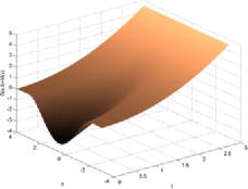
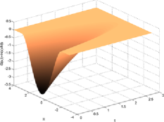
(a)	(b)

Figure 2: We give graphical representations of some of the relevant quantities derived in Example 5.6, for $\alpha=2,\beta=3$ and $\lambda=1/2$. In (a) we see $G(x,t)+H(x)$, which is a lower bound for $F(t)$, and in (b) we see the difference $G(x,t)+H(x)-F(t)$, which is indeed negative.

6 Financial applications

We now turn to our motivating financial problem: consider an asset price $S_{t}$ defined on a complete probability space $(\Omega,\mathcal{F},(\mathcal{F}_{t})_{t\geq 0},\mathbb{P})$, with

$$\frac{\mathrm{d}S_{t}}{S_{t}}=r_{t}\,\mathrm{d}t+\sigma_{t}\,\mathrm{d}W_{t}$$ (48)

under some probability measure $\mathbb{Q}\sim\mathbb{P}$, where $\mathbb{P}$ is the objective probability measure, and $W_{t}$ a $\mathbb{Q}$-Brownian motion. In addition, we suppose $r_{t}$ is the risk-free rate which we require to be known, but which need not be constant. In particular, let $r_{t},\sigma_{t}$ be locally bounded, predictable processes so that the integral in (48) is well defined, and so $S_{t}$ is an Itô process. We suppose that the process $\sigma_{t}$ is not known (or more specifically, we aim to produce conclusions which hold for all $\sigma_{t}$ in the class described). Specifically, we shall suppose:

Assumption 6.1.

The asset price process, under some probability measure $\mathbb{Q}\sim\mathbb{P}$, is the solution to the SDE (48), where $r_{t}$ and $\sigma_{t}$ are locally bounded, predictable processes.

In addition, we need to make the following assumptions regarding the set of call options, which are initially traded:

Assumption 6.2.

We suppose that call options with maturity $T$, and at all strikes $\{K\dvtx K\geq 0\}$ are traded at time $0$, and the prices, $C(K)$, are assumed to be known. In addition, we suppose call-put parity holds, so that the price of a put option with strike $K$ is $P(K)=e^{-\int_{0}^{T}r_{s}\,\mathrm{d}s}K-S_{0}+C(K)$. We make the additional assumptions that $C(K)$ is a continuous, decreasing and convex function, with $C(0)=S_{0}$, $C_{+}^{\prime}(0)=-e^{-\int_{0}^{T}r_{s}\,\mathrm{d}s}$ and $C(K)\to 0$ as $K\to\infty$.

Many of these notions can be motivated by arbitrage concerns; see, for example, Cox and Obłój CoxObloj11 . That there are plausible situations in which these assumptions do not hold can be seen by considering models with bubbles (e.g., CoxHobson05 ), in which call-put parity fails, and $C(K)\not\to 0$ as $K\to\infty$. Let us define $B_{t}=e^{\int_{0}^{t}r_{s}\,\mathrm{d}s}$, and make the assumptions above. Following the perspective that the prices correspond to expectations under $\mathbb{Q}$, the implied law of $B_{T}^{-1}S_{T}$ (which we will denote $\mu$) can be recovered by the Breeden–Litzenberger formula BreedenLitzenberger78 ,

$$\mu((K,\infty))=\mathbb{Q}^{*}\bigl{(}B_{T}^{-1}S_{T}\in(K,\infty)\bigr{)}=-2B_{T}C_{+}^{\prime}(B_{T}K).$$ (49)

Here we have used $\mathbb{Q}^{*}$ to emphasize the fact that this is only an implied probability, and not necessarily the distribution under the actual measure $\mathbb{Q}$. From (49) we deduce that $\mathrm{U}_{\mu}(x)=S_{0}-2C(B_{T}x)-x$, giving an affine mapping between the function $\mathrm{U}_{\mu}(x)$ and the call prices. We do not impose the condition that the law of $B_{T}^{-1}S_{T}$ under $\mathbb{Q}$ is $\mu$, we merely note that this is the law implied by the traded options. We also do not assume anything about the price paths of the call options: our only assumptions are their initial prices, and that they return the usual payoff at maturity. It can now also be seen that the assumption that $C_{+}^{\prime}(0)=-B_{T}^{-1}$ is equivalent to assuming that there is no atom at 0—that is, $\mu$ is supported on $(0,\infty)$. Finally, it follows from the assumptions that $\mu$ is an integrable measure with mean $S_{0}$.

Our goal is to now to use the knowledge of the call prices to find a lower bound on the price of an option which has payoff

$$F\biggl{(}\int_{0}^{T}\sigma_{t}^{2}\,\mathrm{d}t\biggr{)}=F(\langle\ln S\rangle_{T}).$$

Consider the discounted stock price,

$$X_{t}=e^{-\int_{0}^{t}r_{s}\,\mathrm{d}s}S_{t}=B_{t}^{-1}S_{t}.$$

Under Assumption 6.1, $X_{t}$ satisfies the SDE

$$\mathrm{d}X_{t}=X_{t}\sigma_{t}\,\mathrm{d}W_{t}.$$

Defining a time change $\tau_{t}=\int_{0}^{t}\sigma_{s}^{2}\,\mathrm{d}s$, and writing $A_{t}$ for the right-continuous inverse, so that $\tau_{A_{t}}=t$, we note that $\widetilde{W}_{t}=\int_{0}^{A_{t}}\sigma_{s}\,\mathrm{d}W_{s}$ is a Brownian motion with respect to the filtration $\widetilde{\mathcal{F}}_{t}=\mathcal{F}_{A_{t}}$, and if we set $\widetilde{X}_{t}=X_{A_{t}}$, we have

$$\mathrm{d}\widetilde{X}_{t}=\widetilde{X}_{t}\,\mathrm{d}\widetilde{W}_{t}.$$

In particular, $\widetilde{X}_{t}$ is now of a form where we may apply our earlier results, using the target distribution arising from (49), and noting also that $\widetilde{X}_{0}=S_{0}$ and $\widetilde{X}_{\tau_{T}}=X_{T}=B_{T}^{-1}S_{T}$.

We now define functions as in Section 5, so that $f(t)=F_{+}^{\prime}(t)$ and (32)–(36) hold. Our aim is to use (37), which now reads

$$\qquad G(X_{A_{t}},t)+H(X_{A_{t}})=G(\widetilde{X}_{t},t)+H(\widetilde{X}_{t})\leq F(t)=F\biggl{(}\int_{0}^{A_{t}}\sigma_{s}^{2}\,\mathrm{d}s\biggr{)},$$ (50)

to construct a sub-replicating portfolio. We shall first show that we can construct a trading strategy that sub-replicates the $G(\widetilde{X}_{t},t)$ portion of the portfolio. Then we argue that we are able, using a portfolio of calls, puts, cash and the underlying, to replicate the payoff $H(X_{T})$.

Since $G(\widetilde{X}_{t},t)$ is a submartingale, we do not expect to be able to replicate this in a completely self-financing manner. However, by the Doob–Meyer decomposition theorem, and the martingale representation theorem, we can certainly find some process $\widetilde{\phi}_{t}$ such that

$$G(\widetilde{X}_{t},t)\geq G(\widetilde{X}_{0},0)+\int_{0}^{t}\widetilde{\phi}_{s}\,\mathrm{d}\widetilde{X}_{s}$$

and such that there is equality at $t=\tau_{D}$. Moreover, since $G(\widetilde{X}_{\tau_{D}\wedge t},\tau_{D}\wedge t)$ is a martingale, and $G$ is $C^{2,1}$ in $D$, we have

$$G(\widetilde{X}_{\tau_{D}\wedge t},\tau_{D}\wedge t)=G(\widetilde{X}_{0},0)+\int_{0}^{\tau_{D}\wedge t}\frac{\partial G}{\partial x}(\widetilde{X}_{\tau_{D}\wedge s},\tau_{D}\wedge s)\,\mathrm{d}\widetilde{X}_{s}.$$

More generally, we would not expect $\frac{\partial G}{\partial x}$ to exist everywhere in $D^{\complement}$; however, if, for example, left and right derivatives exist, then we could choose $\widetilde{\phi}_{t}\in[\frac{\partial G}{\partial x}(x-,t),\frac{\partial G}{\partial x}(x+,t)]$ as our holding of the risky asset (or alternatively, but less explicitly, take $\widetilde{\phi}_{t}=\partial/\partial x[\mathbb{E}^{x,t}G(\widetilde{X}_{t+\delta},t_{0}+\delta)]$, for $t\in[t_{0},t_{0}+\delta]$).

It follows that we can identify a process $\widetilde{\phi}_{t}$ with

$$G(\widetilde{X}_{\tau_{t}},\tau_{t})\geq G(\widetilde{X}_{0},0)+\int_{0}^{\tau_{t}}\widetilde{\phi}_{s}\,\mathrm{d}\widetilde{X}_{s}=G(X_{0},0)+\int_{0}^{t}\widetilde{\phi}_{\tau_{s}}\,\mathrm{d}X_{s},$$

where we have used, for example, Revuz and Yor RevuzYor99 , Proposition V.1.4. Finally, writing $\phi_{s}=\widetilde{\phi}_{\tau_{s}}$, we have

$$G(X_{t},\tau_{t})\geq G(X_{0},0)+\int_{0}^{t}\phi_{s}\,\mathrm{d}X_{s}=G(X_{0},0)+\int_{0}^{t}\phi_{s}\,\mathrm{d}(B_{s}^{-1}S_{s}).$$

If we consider the self-financing portfolio which consists of holding $\phi_{s}B_{T}^{-1}$ units of the risky asset, and an initial investment of $G(X_{0},0)B^{-1}_{T}-\phi_{0}S_{0}B_{T}^{-1}$ in the risk-free asset, this has value $V_{t}$ at time $t$, where

$$\mathrm{d}(B_{t}^{-1}V_{t})=B_{T}^{-1}\phi_{t}\,\mathrm{d}(B_{t}^{-1}S_{t}),$$

and therefore

$$V_{T}=B_{T}\biggl{(}V_{0}B_{0}^{-1}+\int_{0}^{T}B_{T}^{-1}\phi_{s}\,\mathrm{d}(B_{s}^{-1}S_{s})\biggr{)}=G(X_{0},0)+\int_{0}^{T}\phi_{s}\,\mathrm{d}X_{s}.$$

We now turn to the $H(X_{T})$ component in (50). If $H(x)$ can be written as the difference of two convex functions (so, in particular, $H^{\prime\prime}(\mathrm{d}K)$ is a well-defined signed measure), we can write

$$H(x) = H(S_{0})+H_{+}^{\prime}(S_{0})(x-S_{0})+\int_{(S_{0},\infty)}(x-K)_{+}H^{\prime\prime}(\mathrm{d}K)$$

$${}+\int_{(0,S_{0}]}(K-x)_{+}H^{\prime\prime}(\mathrm{d}K).$$

Taking $x=X_{T}=B_{T}^{-1}S_{T}$, we get

$$H(X_{T}) = H(S_{0})+H_{+}^{\prime}(S_{0})(B_{T}^{-1}S_{T}-S_{0})+B_{T}^{-1}\int_{(S_{0},\infty)}(S_{T}-B_{T}K)_{+}H^{\prime\prime}(\mathrm{d}K)$$

$${}+B_{T}^{-1}\int_{(0,S_{0}]}(B_{T}K-S_{T})_{+}H^{\prime\prime}(\mathrm{d}K).$$

This implies that the payoff $H(X_{T})$ can be replicated at time $T$ by “holding” a portfolio of

$$B_{T}^{-1}\bigl{(}H(S_{0})-H_{+}^{\prime}(S_{0})S_{0}\bigr{)}\mbox{ in cash;}$$

$$B_{T}^{-1}H_{+}^{\prime}(S_{0})\mbox{ units of the asset;}$$

(51)

$$B_{T}^{-1}H^{\prime\prime}(\mathrm{d}K)\mbox{ units of the call with strike }B_{T}K\mbox{ for }K\in(S_{0},\infty);$$

$$B_{T}^{-1}H^{\prime\prime}(\mathrm{d}K)\mbox{ units of the put with strike }B_{T}K\mbox{ for }K\in(0,S_{0}];$$

where the final two terms should be interpreted appropriately. In practice, the function $H(\cdot)$ can typically be approximated by a piecewise linear function, where the “kinks” in the function correspond to traded strikes of calls or puts, in which case the number of units of each option to hold is determined by the change in the gradient at the relevant strike. The initial cost of setting up such a portfolio is well defined, provided

$$\int_{(0,S_{0}]}P(B_{T}K)|H^{\prime\prime}|(\mathrm{d}K)+\int_{(S_{0},\infty)}C(B_{T}K)|H^{\prime\prime}|(\mathrm{d}K)<\infty,$$ (52)

where $|H^{\prime\prime}|(\mathrm{d}K)$ is the total variation of the signed measure $H^{\prime\prime}(\mathrm{d}K)$. We therefore shall make the following assumption:

Assumption 6.3.

The payoff $H(X_{T})$ can be replicated using a suitable portfolio of call and put options, cash and the underlying, with a finite price at time 0.

We can therefore combine these to get the following theorem:

Theorem 6.4

Suppose that Assumptions 6.1, 6.2 and 6.3 hold, and suppose $F(\cdot)$ is a convex, increasing function with $F(0)=0$ and right derivative $f(t)=F_{+}^{\prime}(t)$ which is bounded. Then there exists an arbitrage if the price of an option with payoff $F(\langle\ln S\rangle_{T})$ is less than

$$B_{T}^{-1}G(S_{0},0)+B_{T}^{-1}H(S_{0})+B_{T}^{-1}\int_{(S_{0},\infty)}C(B_{T}K)H^{\prime\prime}(\mathrm{d}K)$$

$$\qquad{}+B_{T}^{-1}\int_{(0,S_{0}]}P(B_{T}K)H^{\prime\prime}(\mathrm{d}K),$$

where the functions $G$ and $H$ are as defined in (35) and (36), and are determined by the solution $\tau_{D}$ to SEP$(\sigma,\delta_{S_{0}},\mu)$ for $\sigma(x)=x$, and where $\mu$ is determined by (49).

Moreover, this bound is optimal in the sense that there exists a model which is free of arbitrage, under which the bound can be attained.

It follows from Theorem 4.6 that, given $\mu$, we can find a domain $D$ and corresponding stopping time $\tau_{D}$ which solves SEP$(\sigma,\delta_{S_{0}},\mu)$. Applying Proposition 5.1 (and bearing in mind Remark 5.5), we conclude that the strategy described above will indeed sub-replicate, and we can therefore produce an arbitrage by purchasing the option, and selling short the portfolio of calls, puts and the underlying given in (6), and in addition, holding the dynamic portfolio with $-\phi_{t}B_{T}^{-1}$ units of the underlying at time $t$. It is not hard to check, given that $f$ is bounded (and choosing the lower limits in (34) to be $S_{0}$ rather than $0$) that $(Z^{\prime}(\widetilde{X}_{s})\sigma(\widetilde{X}_{s}))^{2}\leq(\widetilde{X}_{s}/\widetilde{X}_{0}-1)^{2}$, and hence that (38) holds. Condition (33) also clearly holds. As a consequence, we do indeed have a subhedge.

To see that this is the best possible bound, we need to show that there is a model which satisfies Assumption 6.1, has law $\mu$ under $\mathbb{Q}$ at time $T$, and such that the subhedge is actually a hedge. But consider the stopping time $\tau_{D}$ for the process $\widetilde{X}_{t}$. Define the process

$$X_{t}=\widetilde{X}_{{t}/{(T-t)}\wedge\tau_{D}}\qquad\mbox{for }t\in[0,T]$$

which corresponds to the choice of $\sigma_{s}^{2}=\frac{T-s+1}{(T-t)^{2}}\mathbf{1}_{\{{s}/{(T-s)}<\tau_{D}\}}$. Since $\tau_{D}<\infty$ a.s., then $X_{T}=\widetilde{X}_{\tau_{D}}$, $\tau_{T}=\tau_{D}$ and $S_{t}=X_{t}B_{t}$ is a price process satisfying Assumption 6.1 with

$$F\biggl{(}\int_{0}^{T}\sigma_{t}^{2}\,\mathrm{d}t\biggr{)}=F(\tau_{D}).$$

Finally, it follows from (5) that at time $T$, the value of the hedging portfolio exactly equals the payoff of the option.

Remark 6.5.

The above results are given in the context of an increasing, convex function, but there is also a similar result concerning increasing, concave functions which can be derived. Consider a bounded, increasing function $f$ as before, and define the function

$$L(t)=\int_{0}^{t}\bigl{(}f(\infty)-f(s)\bigr{)}\,\mathrm{d}s=f(\infty)t-F(t).$$

Using Theorem 6.4 and (2), it is easy to see that the price of a contract with payoff $L(\langle\ln S\rangle_{T})$ must be bounded above by

$$2f(\infty)Q-2f(\infty)B_{T}^{-1}\log(S_{0})-B_{T}^{-1}G(S_{0},0)-B_{T}^{-1}H(S_{0})$$

$$\qquad{}-B_{T}^{-1}\int_{(S_{0},\infty)}C(B_{T}K)H^{\prime\prime}(\mathrm{d}K)-B_{T}^{-1}\int_{(0,S_{0}]}P(B_{T}K)H^{\prime\prime}(\mathrm{d}K),$$

where $Q$ is the price of a log-contract [i.e., an option with payoff $\ln(S_{T})$]. As before, this upper bound is the best possible, under a similar set of assumptions.

Remark 6.6.

An analogous result can be shown for forward start options. Suppose that the option has payoff

$$F\biggl{(}\int_{S}^{T}\sigma_{t}^{2}\,\mathrm{d}t\biggr{)}=F(\langle S\rangle_{T}-\langle S\rangle_{S})$$

for fixed times $0<S<T$. Then we can use the previous results for general starting distributions to deduce a similar result to Theorem 6.4 for forward start options, provided we assume that there are calls traded at both $S$ and $T$. We use essentially the same idea as above: we aim to hold a portfolio which (sub-)replicates $G(X_{t},\tau_{t})$ for $t\in[S,T]$, and hold the payoff $H(X_{T})$ as a portfolio of calls. However, we now have $\tau_{t}=\int_{S}^{t}\sigma_{s}^{2}\,\mathrm{d}s$, and so $\widetilde{X}_{t}=X_{A_{t}}$, gives $\widetilde{X}_{0}=X_{S}$ (recall that $A_{t}$ was assumed right-continuous). The procedure is much as above, except that we need to use the solution to Theorem 5.3 with a general target distribution, and the amount $G(\widetilde{X}_{0},0)$ will be a $\mathcal{F}_{S}$-random variable. The initial distribution $\nu$ can be derived using the Breeden–Litzenberger formula (49) at time $S$. To ensure that we hold the amount $G(\widetilde{X}_{0},0)$ at time $S$, we observe that $G(\widetilde{X}_{0},0)=G(X_{S},0)$. Hence if, for example, $G(x,0)$ can be written as the difference of two convex functions, we can replicate this amount by holding a portfolio of calls and puts with maturity $S$ in a similar manner to (6). The remaining details follow as in the hedge described in Theorem 6.4

Remark 6.7.

We can also consider modifications to the realized variance. Consider a slightly different time-change: suppose we set

$$\tau_{t}=\int_{0}^{t}\sigma_{s}^{2}\lambda(X_{s})\,\mathrm{d}s,$$

for some “nice” function $\lambda(x)$, which in particular we suppose is bounded above and below by positive constants. Then following the computations above, we see that

$$\widetilde{X}_{t}=X_{A_{t}}=\int_{0}^{A_{t}}X_{s}\lambda(X_{s})^{-1/2}(\sigma_{s}\lambda(X_{s})^{1/2}\,\mathrm{d}W_{s})=\int_{0}^{t}X_{A_{s}}\lambda(X_{A_{s}})^{-1/2}\,\mathrm{d}\widetilde{W}_{s},$$

and therefore $\mathrm{d}\widetilde{X}_{t}=\sigma(\widetilde{X}_{t})\,\mathrm{d}\widetilde{W}_{t}$, where $\sigma(x)=x\lambda(x)^{-1/2}$. We then conjecture that it is possible to extend Theorem 4.6 to cover this new class of functions $\sigma(x)$ (the conditions that should be imposed on $\lambda$ such that this result may be extended remains an interesting question for future research). It would then be possible to modify the above arguments to provide robust hedges on convex payoffs of the form

$$F\biggl{(}\int_{0}^{T}\sigma_{s}^{2}\lambda(X_{s})\,\mathrm{d}s\biggr{)}.$$

An interesting special case of this would then be to give robust bounds on the price of an option on corridor variance

$$F\biggl{(}\int_{0}^{T}\sigma_{s}^{2}\mathbf{1}_{\{S_{s}\in[a,b]\}}\,\mathrm{d}s\biggr{)},$$ (54)

by considering $\lambda(x)=\mathbf{1}_{\{x\in[a,b]\}}$, however this would only work in the case where there are no discount rates (i.e., $B_{t}=1$). In general, we can only give a tight lower bound for options on

$$F\biggl{(}\int_{0}^{T}\sigma_{s}^{2}\mathbf{1}_{\{X_{s}\in[\widetilde{a},\widetilde{b}]\}}\,\mathrm{d}s\biggr{)},$$

although this does provide a lower bound for (54) by considering the case where $\widetilde{a}=a$ and $\widetilde{b}=B_{T}b$.

7 Conclusions

We conclude by summarizing the results, and describing some interesting questions for future work. In this paper, we have given a variational inequality representation of Root’s solution to the Skorokhod embedding problem, and provided a novel proof of optimality, which allows us to construct a model-independent subhedge for options on variance. We believe that our results provide interesting insights into all three aspects of the work: the construction of solutions to the Skorokhod embedding problem, proving optimality results for the same and finally the connections with model-independent hedging.

We also believe that there are interesting lines of research that now arise. The construction opens up a number of questions regarding Root’s solution to the Skorokhod embedding problem: for example, what can be said about the shape of the boundary? Under what conditions on $\mu$ will the boundary be smooth? When does $R(x)\to 0$ as $x\to\pm\infty$? When is $R(x)$ bounded? Properties of free boundaries are well studied in the analytic literature, and may be useful in answering these questions. The connection to minimality and noncentered target distributions raised in Remark 4.5, and the question asked at the end of this remark would also be interesting lines for research.

The connection with optimal stopping noted in Remark 4.4 is interesting, and obtaining a deeper understanding between optimal stopping problems and optimal Skorokhod embeddings seems to be an interesting area of research.

Another natural question concerns the upper bound/super-hedging strategy. It has been remarked by Obłój Obloj04 and Carr and Lee CarrLee10 that a related construction of Rost should provide a suitable upper bound, but similar questions to those answered here remain (although we hope to be able to provide some answers in subsequent work). We note, however, that numerical evidence (see Carr and Lee CarrLee10 ) seems to suggest that the Root bounds may be more appropriate in the financial applications. It would also be of interest to see to what extent these model-independent bounds may be useful in practice. In Cox and Obłój CoxObloj11 , an analysis of the use of model-independent bounds as a hedging strategy for barrier options was performed. A similar analysis of the strategies derived in this work would also be of interest.

Other questions that arise from the practical standpoint include how to incorporate additional market information (e.g., calls at an intermediate time BrownHobsonRogers01b ), and how to adjust for the fact that there will generally only be a finite set of quoted calls; see DavisOblojRaval10 for a related question. Remark 6.7 also suggests open questions regarding more general choices of $\sigma(x)$.

References

• (1) {bbook}[mr] \bauthor\bsnmBensoussan, \bfnmAlain\binitsA. and \bauthor\bsnmLions, \bfnmJacques-Louis\binitsJ.-L. (\byear1982). \btitleApplications of Variational Inequalities in Stochastic Control. \bseriesStudies in Mathematics and Its Applications \bvolume12. \bpublisherNorth-Holland, \baddressAmsterdam. \bidmr=0653144 \bptokimsref \endbibitem
• (2) {barticle}[author] \bauthor\bsnmBreeden, \bfnmD. T.\binitsD. T. and \bauthor\bsnmLitzenberger, \bfnmR. H.\binitsR. H. (\byear1978). \btitlePrices of state-contingent claims implicit in option prices. \bjournalJournal of Business \bvolume51 \bpages621–651. \bptokimsref \endbibitem
• (3) {barticle}[author] \bauthor\bsnmBroadie, \bfnmM.\binitsM. and \bauthor\bsnmJain, \bfnmA.\binitsA. (\byear2008). \btitlePricing and hedging volatility derivatives. \bjournalThe Journal of Derivatives \bvolume15 \bpages7–24. \bptokimsref \endbibitem
• (4) {barticle}[mr] \bauthor\bsnmBrown, \bfnmHaydyn\binitsH., \bauthor\bsnmHobson, \bfnmDavid\binitsD. and \bauthor\bsnmRogers, \bfnmL. C. G.\binitsL. C. G. (\byear2001). \btitleThe maximum maximum of a martingale constrained by an intermediate law. \bjournalProbab. Theory Related Fields \bvolume119 \bpages558–578. \biddoi=10.1007/PL00008771, issn=0178-8051, mr=1826407 \bptokimsref \endbibitem
• (5) {barticle}[mr] \bauthor\bsnmCarr, \bfnmPeter\binitsP. and \bauthor\bsnmLee, \bfnmRoger\binitsR. (\byear2010). \btitleHedging variance options on continuous semimartingales. \bjournalFinance Stoch. \bvolume14 \bpages179–207. \biddoi=10.1007/s00780-009-0110-3, issn=0949-2984, mr=2607762 \bptokimsref \endbibitem
• (6) {barticle}[author] \bauthor\bsnmCarr, \bfnmP.\binitsP., \bauthor\bsnmLee, \bfnmR.\binitsR. and \bauthor\bsnmWu, \bfnmL.\binitsL. (\byear2012). \btitleVariance swaps on time-changed Lévy processes. \bjournalFinance Stoch. \bvolume16 \bpages335–355. \bidmr=2903628 \bptokimsref \endbibitem
• (7) {barticle}[mr] \bauthor\bsnmChacon, \bfnmR. V.\binitsR. V. (\byear1977). \btitlePotential processes. \bjournalTrans. Amer. Math. Soc. \bvolume226 \bpages39–58. \bidissn=0002-9947, mr=0501374 \bptokimsref \endbibitem
• (8) {bincollection}[mr] \bauthor\bsnmCox, \bfnmA. M. G.\binitsA. M. G. (\byear2008). \btitleExtending Chacon–Walsh: Minimality and generalised starting distributions. In \bbooktitleSéminaire de Probabilités XLI. \bseriesLecture Notes in Math. \bvolume1934 \bpages233–264. \bpublisherSpringer, \baddressBerlin. \biddoi=10.1007/978-3-540-77913-1_12, mr=2483735 \bptokimsref \endbibitem
• (9) {barticle}[mr] \bauthor\bsnmCox, \bfnmAlexander M. G.\binitsA. M. G. and \bauthor\bsnmHobson, \bfnmDavid G.\binitsD. G. (\byear2005). \btitleLocal martingales, bubbles and option prices. \bjournalFinance Stoch. \bvolume9 \bpages477–492. \biddoi=10.1007/s00780-005-0162-y, issn=0949-2984, mr=2213778 \bptokimsref \endbibitem
• (10) {barticle}[mr] \bauthor\bsnmCox, \bfnmA. M. G.\binitsA. M. G., \bauthor\bsnmHobson, \bfnmDavid G.\binitsD. and \bauthor\bsnmObłój, \bfnmJan\binitsJ. (\byear2008). \btitlePathwise inequalities for local time: Applications to Skorokhod embeddings and optimal stopping. \bjournalAnn. Appl. Probab. \bvolume18 \bpages1870–1896. \biddoi=10.1214/07-AAP507, issn=1050-5164, mr=2462552 \bptokimsref \endbibitem
• (11) {barticle}[mr] \bauthor\bsnmCox, \bfnmAlexander M. G.\binitsA. M. G. and \bauthor\bsnmObłój, \bfnmJan\binitsJ. (\byear2011). \btitleRobust pricing and hedging of double no-touch options. \bjournalFinance Stoch. \bvolume15 \bpages573–605. \biddoi=10.1007/s00780-011-0154-z, issn=0949-2984, mr=2833100 \bptokimsref \endbibitem
• (12) {barticle}[mr] \bauthor\bsnmCox, \bfnmA. M. G.\binitsA. M. G. and \bauthor\bsnmObłój, \bfnmJan\binitsJ. (\byear2011). \btitleRobust hedging of double touch barrier options. \bjournalSIAM J. Financial Math. \bvolume2 \bpages141–182. \biddoi=10.1137/090777487, issn=1945-497X, mr=2772387 \bptokimsref \endbibitem
• (13) {bmisc}[author] \bauthor\bsnmDavis, \bfnmM. H. A.\binitsM. H. A., \bauthor\bsnmObłój, \bfnmJ.\binitsJ. and \bauthor\bsnmRaval, \bfnmV.\binitsV. (\byear2010). \bhowpublishedArbitrage bounds for weighted variance swap prices. Available at http://arxiv.org/abs/1001.2678. \bptokimsref \endbibitem
• (14) {bincollection}[mr] \bauthor\bsnmDinges, \bfnmH.\binitsH. (\byear1974). \btitleStopping sequences. In \bbooktitleSéminaire de Probabilitiés, VIII (Univ. Strasbourg, Année Universitaire 1972–1973). \bseriesLecture Notes in Math. \bvolume381 \bpages27–36. \bpublisherSpringer, \baddressBerlin. \bidmr=0383552 \bptokimsref \endbibitem
• (15) {barticle}[author] \bauthor\bsnmDupire, \bfnmB.\binitsB. (\byear1993). \btitleModel art. \bjournalRisk \bvolume6 \bpages118–120. \bptokimsref \endbibitem
• (16) {bmisc}[author] \bauthor\bsnmDupire, \bfnmB.\binitsB. (\byear2005). \bhowpublishedArbitrage bounds for volatility derivatives as free boundary problem. Presentation at “PDE and Mathematical Finance,” KTH, Stockholm. \bptokimsref \endbibitem
• (17) {bbook}[mr] \bauthor\bsnmFriedman, \bfnmAvner\binitsA. (\byear1963). \btitleGeneralized Functions and Partial Differential Equations. \bpublisherPrentice-Hall Inc., \baddressEnglewood Cliffs, NJ. \bidmr=0165388 \bptokimsref \endbibitem
• (18) {barticle}[author] \bauthor\bsnmHobson, \bfnmDavid G.\binitsD. G. (\byear1998). \btitleRobust hedging of the lookback option. \bjournalFinance Stoch. \bvolume2 \bpages329–347. \bptokimsref \endbibitem
• (19) {bincollection}[mr] \bauthor\bsnmHobson, \bfnmDavid\binitsD. (\byear2011). \btitleThe Skorokhod embedding problem and model-independent bounds for option prices. In \bbooktitleParis–Princeton Lectures on Mathematical Finance 2010 (\beditor\bfnmR. A.\binitsR. A. \bsnmCarmona, \beditor\bfnmE.\binitsE. \bsnmÇinlar, \beditor\bfnmI.\binitsI. \bsnmEkeland, \beditor\bfnmE.\binitsE. \bsnmJouini, \beditor\bfnmJ. A.\binitsJ. A. \bsnmScheinkman and \beditor\bfnmN.\binitsN. \bsnmTouzi, eds.). \bseriesLecture Notes in Math. \bvolume2003 \bpages267–318. \bpublisherSpringer, \baddressBerlin. \biddoi=10.1007/978-3-642-14660-2_4, mr=2762363 \bptnotecheck year\bptokimsref \endbibitem
• (20) {barticle}[author] \bauthor\bsnmHowison, \bfnmS.\binitsS., \bauthor\bsnmRafailidis, \bfnmA.\binitsA. and \bauthor\bsnmRasmussen, \bfnmH.\binitsH. (\byear2004). \btitleOn the pricing and hedging of volatility derivatives. \bjournalAppl. Math. Finance \bvolume11 \bpages317. \bptokimsref \endbibitem
• (21) {barticle}[mr] \bauthor\bsnmKallsen, \bfnmJan\binitsJ., \bauthor\bsnmMuhle-Karbe, \bfnmJohannes\binitsJ. and \bauthor\bsnmVoß, \bfnmMoritz\binitsM. (\byear2011). \btitlePricing options on variance in affine stochastic volatility models. \bjournalMath. Finance \bvolume21 \bpages627–641. \biddoi=10.1111/j.1467-9965.2010.00447.x, issn=0960-1627, mr=2838578 \bptokimsref \endbibitem
• (22) {bmisc}[author] \bauthor\bsnmKeller-Ressel, \bfnmM.\binitsM. (\byear2011). \bhowpublishedConvex order properties of discrete realized variance and applications to variance options. Available at http://arxiv.org/ abs/1103.2310. \bptokimsref \endbibitem
• (23) {bmisc}[author] \bauthor\bsnmKeller-Ressel, \bfnmM.\binitsM. and \bauthor\bsnmMuhle-Karbe, \bfnmJ.\binitsJ. (\byear2010). \bhowpublishedAsymptotic and exact pricing of options on variance. Available at http://arxiv.org/abs/1003.5514. \bptokimsref \endbibitem
• (24) {barticle}[mr] \bauthor\bsnmLoynes, \bfnmR. M.\binitsR. M. (\byear1970). \btitleStopping times on Brownian motion: Some properties of Root’s construction. \bjournalZ. Wahrsch. Verw. Gebiete \bvolume16 \bpages211–218. \bidmr=0292170 \bptokimsref \endbibitem
• (25) {barticle}[mr] \bauthor\bsnmMonroe, \bfnmItrel\binitsI. (\byear1972). \btitleOn embedding right continuous martingales in Brownian motion. \bjournalAnn. Math. Statist. \bvolume43 \bpages1293–1311. \bidissn=0003-4851, mr=0343354 \bptokimsref \endbibitem
• (26) {barticle}[author] \bauthor\bsnmNeuberger, \bfnmA.\binitsA. (\byear1994). \btitleThe log contract. \bjournalThe Journal of Portfolio Management \bvolume20 \bpages74–80. \bptokimsref \endbibitem
• (27) {barticle}[mr] \bauthor\bsnmObłój, \bfnmJan\binitsJ. (\byear2004). \btitleThe Skorokhod embedding problem and its offspring. \bjournalProbab. Surv. \bvolume1 \bpages321–390. \biddoi=10.1214/154957804100000060, issn=1549-5787, mr=2068476 \bptokimsref \endbibitem
• (28) {bincollection}[mr] \bauthor\bsnmObłój, \bfnmJan\binitsJ. (\byear2007). \btitleThe maximality principle revisited: On certain optimal stopping problems. In \bbooktitleSéminaire de Probabilités XL. \bseriesLecture Notes in Math. \bvolume1899 \bpages309–328. \bpublisherSpringer, \baddressBerlin. \biddoi=10.1007/978-3-540-71189-6_16, mr=2409013 \bptokimsref \endbibitem
• (29) {barticle}[mr] \bauthor\bsnmPeskir, \bfnmGoran\binitsG. (\byear1998). \btitleOptimal stopping of the maximum process: The maximality principle. \bjournalAnn. Probab. \bvolume26 \bpages1614–1640. \biddoi=10.1214/aop/1022855875, issn=0091-1798, mr=1675047 \bptokimsref \endbibitem
• (30) {bbook}[mr] \bauthor\bsnmProtter, \bfnmPhilip E.\binitsP. E. (\byear2005). \btitleStochastic Integration and Differential Equations, \bedition2nd ed. \bseriesStochastic Modelling and Applied Probability \bvolume21. \bpublisherSpringer, \baddressBerlin. \bptokimsref \endbibitem
• (31) {bbook}[mr] \bauthor\bsnmRevuz, \bfnmDaniel\binitsD. and \bauthor\bsnmYor, \bfnmMarc\binitsM. (\byear1999). \btitleContinuous Martingales and Brownian Motion, \bedition3rd ed. \bseriesGrundlehren der Mathematischen Wissenschaften [Fundamental Principles of Mathematical Sciences] \bvolume293. \bpublisherSpringer, \baddressBerlin. \bidmr=1725357 \bptokimsref \endbibitem
• (32) {bbook}[mr] \bauthor\bsnmRogers, \bfnmL. C. G.\binitsL. C. G. and \bauthor\bsnmWilliams, \bfnmDavid\binitsD. (\byear2000). \btitleDiffusions, Markov Processes, and Martingales. Vol. 2. \bpublisherCambridge Univ. Press, \baddressCambridge. \bidmr=1780932 \bptokimsref \endbibitem
• (33) {barticle}[mr] \bauthor\bsnmRoot, \bfnmD. H.\binitsD. H. (\byear1969). \btitleThe existence of certain stopping times on Brownian motion. \bjournalAnn. Math. Statist. \bvolume40 \bpages715–718. \bidissn=0003-4851, mr=0238394 \bptokimsref \endbibitem
• (34) {barticle}[mr] \bauthor\bsnmRost, \bfnmHermann\binitsH. (\byear1971). \btitleThe stopping distributions of a Markov Process. \bjournalInvent. Math. \bvolume14 \bpages1–16. \bidissn=0020-9910, mr=0346920 \bptokimsref \endbibitem
• (35) {bincollection}[mr] \bauthor\bsnmRost, \bfnmH.\binitsH. (\byear1976). \btitleSkorokhod stopping times of minimal variance. In \bbooktitleSéminaire de Probabilités, X (Première Partie, Univ. Strasbourg, Strasbourg, Année Universitaire 1974/1975) \bseriesLecture Notes in Math. \bvolume511 \bpages194–208. \bpublisherSpringer, \baddressBerlin. \bidmr=0445600 \bptokimsref \endbibitem
• (36) {bbook}[mr] \bauthor\bsnmStroock, \bfnmDaniel W.\binitsD. W. (\byear2008). \btitlePartial Differential Equations for Probabilists. \bseriesCambridge Studies in Advanced Mathematics \bvolume112. \bpublisherCambridge Univ. Press, \baddressCambridge. \biddoi=10.1017/CBO9780511755255, mr=2410225 \bptokimsref \endbibitem