Radial stability analysis of the continuous pressure gravastar
Abstract
Radial stability of the continuous pressure gravastar is studied using the conventional Chandrasekhar method. The equation of state for the static gravastar solutions is derived and Einstein equations for small perturbations around the equilibrium are solved as an eigenvalue problem for radial pulsations. Within the model there exist a set of parameters leading to a stable fundamental mode, thus proving radial stability of the continuous pressure gravastar. It is also shown that the central energy density possesses an extremum in curve which represents a splitting point between stable and unstable gravastar configurations. As such the curve for the gravastar mimics the famous curve for a polytrope. Together with the former axial stability calculations this work completes the stability problem of the continuous pressure gravastar.
I Introduction
Gravitational collapse as the stellar nuclear fuel is consumed could lead to black holes - objects which are accepted by scientific community but their undesired and even paradoxical features (singularities, horizon) have motivated research in a direction of finding massive objects (stars) without singularities and without horizon. One of these alternatives is a gravastar.
Since the seminal work of Mazur and Mottola MazurMottola the concept of the gravitational vacuum star – the gravastar – as an alternative to a black hole has attracted a plethora of interest. In this version of the gravastar a multilayered structure has been introduced: from the repulsive de Sitter core (where a negative pressure helps balance the collapsing matter) one crosses multiple layers (shells) and without encountering a horizon one eventually reaches the (pressureless) exterior Schwarzschild spacetime. Later some simplifications Carter ; Visser and modifications Lobo:StableDES have been introduced in the original (multi)layer - onion-like picture.
An important step was done when it was shown that due to anisotropy of matter comprising the gravastar Cattoen one can eliminate layer(s) and, by a continuous stress-energy tensor, the transition from the interior de Sitter spacetime segment to the exterior Schwarzschild spacetime is possible DeBenedictis (see also Dymnikova ). The pressure anisotropy in the spherically symmetric geometry was perhaps first introduced by G. Lemaître Lemaitre and suggested by Einstein (as quoted in Lemaitre ). The vanishing radial pressure with transversal pressure only was shown to be enough to support a stable object. Further development Bowers-Liang ; Fuzfa-etal has brought different refinements to the original anisotropy notion. The pressure anisotropy, which is shown to be a necessary condition for the existence of a gravastar Cattoen is met also in boson star models Schunck-Mielke and wormholes Garattini . The anisotropy (defined as a difference between the transversal and radial pressure) vanishes at the center () of the star as well as at its boundary (). The gravastar has been confronted with its rivals - black holes DeBenedictisRev ; RochaMCh and wormholes Garattini ; SushkovZaslavski ; DeBenedictisGarLobo , and investigated with respect to energy conditions (violations) HorvatEC and its charged properties Horvat:Charged ; LoboArellano . An interesting question has been posed several times: is it possible to distinguish the gravastar from a black hole HarkoKL ; Rezzolla ; BroderickNarayan ? In Ref. Rezzolla it was shown that gravitational radiation could be used to tell a gravastar from a black hole. However, the definite answer to this question has not been given at satisfactory level and the gravastar research is still a dynamic field with recent papers like Lobo:Noncommutative ; PaniBerti ; BrandtChan ; UsmaniRahaman etc.
Almost every research mentioned above to some extent addresses the problem of the gravastar stability, since the stability problem is crucial for any object or situation to be considered as physically viable. In Ref. MazurMottola it was first shown that such an object is thermodynamically stable, while axial stability of thin-shells gravastars was tested in Carter ; Lobo:StableDES . Stability within the thin shell approach based on the Darmois-Israel formalism was recently reviewed in LoboCrawford . In Rezzolla stability analysis of the thin shell gravastar problem is closely related to an attempt to distinguish the gravastar from a black hole by analysis of quasi-normal modes produced by axial perturbations. Problem of stability of a rotating the thin shell gravastar was addressed in ChirentiRezzolla . Stability in the (multi)layer version of the gravastar was also considered in GasparRacz ; PaniBerti ; PaniCardoso ; RochaMCh .
The axial stability of the continuous pressure gravastar was shown to be valid in DeBenedictis . This analysis was based on the Ref. DymnikovaGalaktionov where stability of objects with de Sitter centers was investigated.
In this paper we analyze the radial stability of the continuous pressure gravastars DeBenedictis following the conventional Chandrasekhar method. Originally Chandrasekhar developed the method for testing the radial stability of the isotropic spheres Chandrasekhar:1964 in terms of the radial pulsations. In Ref. Gleiser:Stability Chandrasekhar’s method was generalized to anisotropic spheres. Stability of anisotropic stars was investigated before in HeintzmannHillebrandt ; Hillebrandt and radial stability analysis for anisotropic stars using the quasi-local equation of state was given in Horvat:Stability . The standard mathematical procedure is here applied to an object with a peculiar behavior of pressures (see below) and although the mathematical rigor was never abandoned, the analysis due to the character of the object could be considered as a toy model analysis of radial stability.
This paper is organized as follows. In the next section the
linearization of the Einstein equations is given. Static solutions
are described, an equation of state is derived and the pulsation
equation is obtained. In Sec. III the eigenvalue problem for the
radial displacement is presented. Results and discussion are given
in the
last section.
Unless stated explicitly we shall work in units where
.
II Linearization of the Einstein equation
In this paper the response of the continuous pressure gravastar model to small radial perturbations is considered. Assuming that the pulsating object retains its spherical symmetry, one can introduce the Schwarzschild coordinates:
| (1) |
where and are, in this dynamical setting, time-dependent metric functions.
The standard anisotropic energy-momentum tensor appropriate to describe continuous pressure gravastars is:
| (2) |
where is the fluid 4-velocity, , and are the unit
4-vectors in the and directions, respectively, .
The velocity of the fluid element in the radial direction
is defined by:
| (3) |
where is the radial displacement of the fluid element, . The components of the 4-velocity are obtained by employing and Eq. (3):
| (4) |
The non-zero components of the energy-momentum tensor (2) linear in are:
| (5) |
The components of the Einstein tensor for the metric (1) are:
| (6) | |||||
| (7) | |||||
| (8) | |||||
| (9) |
Following the standard Chandrasekhar method, all matter and metric functions should only slightly deviate from their equilibrium solutions,
| (10) |
| (11) |
The subscript denotes the equilibrium functions and are the so-called Eulerian perturbations, where . The Eulerian perturbations measure a local departure from equilibrium in contrast to the Lagrangian perturbations, denoted as , which measure a departure from equilibrium in the co-moving system (fluid rest frame). The Lagrangian perturbations in the linear approximation play a role of a total differential and are linked to the Eulerian perturbations via the equation (see e.g. Ref. MTW ):
| (12) |
A linearization of the Einstein equations leads to the two sets of equations: one for the equilibrium (static) functions and the other for the perturbed functions. The equilibrium functions obey the following set of equations:
| (13) | |||||
| (14) | |||||
| (15) |
In practice, one usually combines these three equations into the Tolman-Oppenheimer-Volkoff (TOV) equation:
| (16) |
where denotes the anisotropic term . The other set of equations emerging from the linearization of the above Einstein equations yield the set of equations for the perturbed functions:
| (17) |
| (18) |
| (19) |
| (20) |
Equation (20) is known as the pulsation
equation Gleiser:Stability and it serves to probe the
radial stability of the system of interest. It is actually the TOV
equation for the perturbed functions which is obtained –
analogously as the non-perturbed TOV – by combining Einstein
equations for perturbed functions.
In order to solve the pulsation equation (20) for
the gravastar all perturbed functions should be expressed
in terms of the radial displacement (and its derivatives)
and the equilibrium functions. In performing this, one first
integrates Eq. (19) in time, yielding:
| (21) |
Using this expression for in Eq. (17) one obtains:
| (22) |
After inserting in Eq. (18) a dependence on remains, which should be expressed in terms of the displacement function (and its derivatives) and the equilibrium functions. To accomplish this, one ought to explore the system at hand in more detail.
One of the possibilities, as suggested firstly by Chandrasekhar for isotropic structures Chandrasekhar:1964 and more recently by Dev and Gleiser for anisotropic objects Gleiser:Stability , is to make use of the baryon density conservation to express the radial pressure perturbation in terms of the displacement function and the static solutions. In this approach the adiabatic index appears as a free parameter. Chandrasekhar used this method to establish limiting values of the adiabatic index leading to an (un)stable isotropic object of a constant energy density. He showed that there were no stable stars of this kind if the adiabatic index was less than ( is a constant of order unity depending on the structure of the star, and are the star’s mass and radius). In Ref. Gleiser:Stability the Chandrasekhar method was extended to various anisotropic star models and showed that the limiting value of the adiabatic index is shifted to lower values, i.e. anisotropic stars can approach the stability region with smaller adiabatic index than in the Chandrasekhar’s case.
In this paper our primary concern is to probe the radial stability of one particular anisotropic object – the gravastar. Due to the peculiar character of the gravastar (especially its radial pressure – see below) one cannot expect the adiabatic index to be constant along the whole object. In fact the adiabatic index is a function of the energy density and pressure(s). This is the main reason why in this paper stability will not be tested by fixing the appropriate values of the adiabatic index that guarantee stability. The required information will rather be extracted from a given static solution by constructing the equation of state.
II.1 Static solution
The procedure discussed so far is applicable to all spherically symmetric structures. To apply it to gravastar configurations one has to recall the basic characteristics of gravastars in the continuous pressure picture DeBenedictis . The energy density is positive and monotonically decreases from the center to the surface. Gravastars have a de Sitter-like interior, , and a Schwarzschild-like exterior. Furthermore, the atmosphere of the gravastar is defined as an outer region, near to the surface, where ”normal” physics is valid Cattoen , i.e. where both the energy-density and the radial pressure are positive and monotonically decreasing functions of the radius. In the gravastar’s atmosphere the sound velocity , with
| (23) |
is real () and subluminal ().
From the peculiar shape of the gravastar’s (radial) pressure
one can immediately infer that the sound velocity ought to be real
only in the gravastar’s atmosphere, whilst in the gravastar’s
interior it is imaginary, . This is the main reason
why, in probing the radial stability, we shall be primarily concerned
with the physical processes occurring in the gravastar’s
atmosphere.
To construct a static gravastar, the energy density profile and the anisotropic term are adopted from the previous work DeBenedictis ; Horvat:Charged :
| (24) |
| (25) |
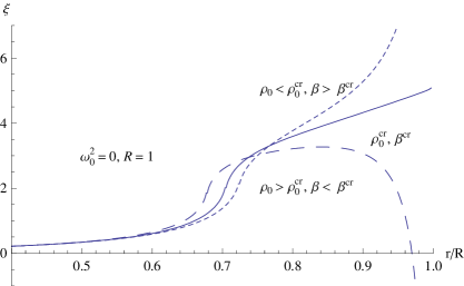
Here , are (free) parameters and is the central energy density. is the anisotropy strength measure and is the radius of the gravastar for which . is the compactness function defined by , where is the mass function . The radial pressure is a solution of the TOV (16) and the tangential pressure is readily obtained from the anisotropy and the radial pressure by employing the identity . The particular form of the anisotropic term is dictated by the behavior of pressures at de Sitter core, since at the anisotropy should vanish as seen from (16). Also, the above form of the anisotropy term ensures that the radial pressure vanishes at . The transversal pressure vanishes as well although it is not necessary to be the case (see Ref. DeBenedictis for the gravastar model with non vanishing transverse pressure.). The anisotropy strength measure is controlled as well by the energy conditions which have to be met.
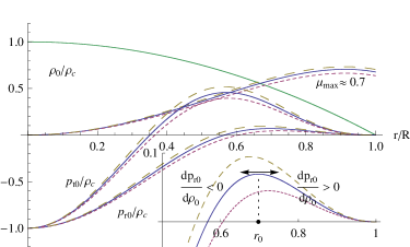
One such solution for fixed is shown in Fig. 1
for three different values of the central energy density
corresponding to three different values of the anisotropy strength
. Since the radius is fixed there is an
interplay between the central energy density and
anisotropy strength – a higher central energy density
requires a smaller anisotropy strength . We shall
elaborate on this particular choice of parameters in Section IV,
where the radial stability of these three gravastar configurations
will be tested.
In the inset of Fig. 1 the radial pressure close to the surface is
extracted in order to show important features of the gravastar’s
atmosphere. At the radius the sound velocity of the fluid
vanishes () and hence serves as
a division point of the propagating (or physically reasonable)
(, ) and non-propagating regions (,
) when
probing radial pulsations of the gravastar.
The dominant energy condition (DEC), i.e. , is obeyed by both radial and tangential pressure
throughout the gravastar. The compactness function has also been
shown in Fig. 1.
II.2 Equation of state
In this subsection we note that the equation of state (EoS)
appropriate to describe the gravastar (inferred from the input
functions (24) and (25)) is actually a
functional of the energy density (only), parameterized by the
anisotropy strength . Next this result is used to compute
the Eulerian perturbation of the radial pressure from
the EoS, by perturbing the energy density only. Ultimately this
completes the task to express all perturbed functions
in terms of the displacement (and its derivatives) and the static solutions.
Generally, for isotropic structures, before solving the TOV, one
assumes that the pressure and the energy density are
functions of the specific entropy and the baryon density .
If a system is described by the one-fluid model, then in static
and dynamic settings it exhibits isentropic behavior (constant
), in which case one can set . Thus it is possible to
eliminate the baryon density and express the pressure in terms
of the energy density only, leading to a barotropic equation of
state .
It is a rather simple task now to perturb this EoS and express the perturbed
pressure in terms of the perturbed energy density.
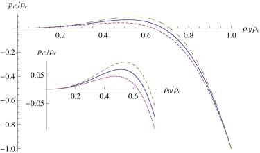
For anisotropic objects the EoS is highly dependent on the anisotropic term model (see e.g. the TOV (16)). The particular choice of the anisotropic term used here (25) is a functional (or a quasi-local variable 444By the quasi-local variable we mean a function which is an integral in space of some local function – for example, the mass function is a quasi-local variable of the energy density (which is a local function) as it is the volume integral of the energy density (the same holds for the compactness function). For a discussion of quasi-local variables and quasi-local EoS see e.g. Refs. Hernandes:Eos ; Hernandez:EoS-aniz and Ref. Horvat:Stability .) of the energy density. This means that for a fixed anisotropy strength there is a two parameter family of values belonging to the same EoS (see Fig. 2). As a consequence, one can obtain perturbed (radial) pressure by perturbing the energy density only, and keeping the anisotropy strength fixed.
To illustrate this in more detail let us introduce an analytic form of the EoS which, to a good approximation, describes the gravastar configuration defined by (24) and (25): 555It is worth noting that the analytic form of the EoS (26) is not restricted to the chosen energy density (24). For example, it is also appropriate to describe a gravastar with the energy density of the form .
| (26) |
Here is closely related to the anisotropy strength , is the compactness function which is a functional of the energy density. Now it is clear that for a fixed the (radial) pressure is fully determined by the energy density.
Hence, following the reasoning outlined above and making use of Eq. (12), in the linear approximation the Eulerian perturbation for the radial pressure is:
| (27) |
Here denotes functional derivative of
the radial pressure with respect to the energy density. This is
equal to as both the radial
pressure and the
energy density are functions of radius only.
Similarly, the Eulerian perturbation of the anisotropy
assumes the form:
| (28) |
With the above two expressions the pulsation equation (20) is fully determined. However, before proceeding to solve the pulsation equation it is useful to rewrite Eq. (27) in a slightly different form in order to compare the result in this paper with that of Chandrasekhar’s for isotropic, and Dev and Gleiser’s for anisotropic stars. By means of the TOV (16) the perturbed energy density (22) can be written as
| (29) |
Inserting this result in Eq. (27) the radial pressure perturbation becomes
| (30) |
If one now identifies the adiabatic ”index” as
| (31) |
the result derived in Eq. (30) reduces to that of Dev and Gleiser Gleiser:Stability , Eq. (86). However, the expressions for differ. Moreover, if one turns off anisotropy () Chandrasekhar’s result is obtained.
III The pulsation equation as an eigenvalue problem
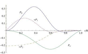
As in the Chandrasekhar method all matter and metric functions exhibit oscillatory behavior in time, . Hence the pulsation equation assumes the form:
| (32) |
where and are polynomial functions of , depending on the static solutions only (see Fig. 3). Eq. (32) represents an eigenvalue equation for the radial displacement (with being an eigenvalue). Solutions of this differential equation are obtained by specifying boundary conditions in the center and at the surface of the gravastar:
| (33) |
| (34) |
The boundary condition in the center demands that there is no displacement of the fluid in the center of the gravastar. The boundary condition at the surface follows from the requirement that the Lagrangian radial pressure perturbation has to vanish at the surface MTW ; Catalogue ; Kokkotas:Oscillation . In the model presented here where , the sound velocity vanishes at the surface, . This means that, apart from being finite, there are no further restrictions on . This also implies that it is sufficient to demand that and are bounded in order to satisfy the boundary condition at the surface Catalogue . The choice
| (35) |
enables one to compare the results in the gravastar’s atmosphere with the radial oscillations of the
polytropes. This can be relevant as the EoS of the gravastar’s atmosphere
close to the surface can be approximated by the polytropic
EoS , where is a polytropic index DeBenedictis ; Horvat:Charged .
In order to study radial stability of the system described by Eq. (20) subject to the boundary
conditions (33) and (34), it is plausible
to recast the pulsation equation into the standard
Sturm-Liouville form (see e.g. Ref. MTW ):
| (36) |
where
| (37) |
The leading coefficient in the pulsation equation has three zeros - two at the ends
and one in the interior region (), hence
has three singular points (see Fig. 3), though all three are regular singular points or Fuchsian
singularities Slavyanov 666A singular point is regular (or Fuchsian) if the function
has a pole of at most first order, and the function has a pole of at most second order
at the singular point ..
In order to obtain the integral should be calculated, and since the interior singularity arises at which is a division point between propagating and non-propagating domains, it is reasonable to divide the whole interval in two parts: and . In performing the integration numerically infinitesimally small regions around all three singular points are excluded, so that both integrals are rendered convergent and finite. As a consequence, the leading coefficient in the Sturm-Liouville equation is a positive function on the (whole) interval , whilst the weight function is negative on the interval and positive on the interval . As elucidated in the previous section, the interesting region is the gravastar’s atmosphere, i.e. the second interval, . In this region the standard Sturm-Liouville eigenvalue problem formalism (see e.g. Catalogue ) is applied, since and . Therefore if is positive, itself is real and the solution is oscillatory. If on the other hand is negative, is imaginary and the solution is exponentially growing or decaying in time, thus signalizing instabilities. The number of nodes of the eigenvector for a given eigenvalue is closely related to the stability criteria. To be more precise, if for eigenvector has no nodes, then all higher frequency radial modes are stable. Otherwise, if for eigenvector exhibits nodes, then all radial modes are unstable. Furthermore, if the system is stable, then the following relations hold
| (38) |
where equals the number of nodes.
IV Results and Discussion
In testing stability of certain configurations in general, it
seems natural that one attempts to find critical values of the
parameters for which the system is marginally stable. Marginal
stability means
here that there exists a set of parameters for which the system
exhibits the stable fundamental mode () for .
Then for the given set of parameters all higher frequency
modes are radially stable. For example, in the case of neutron
stars (described by the polytropic EoS), there exists a critical
value of the central energy density for which the stellar mass
as a function of radius is extremal. For such a critical value
of the central energy density the star exhibits stable fundamental
mode with , which implies that all higher frequency
modes with the given central energy density are then radially
stable. Furthermore, at the account of the curve one can
then read off which configuration of the EoS
will produce a stable star and which will not.
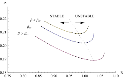
The continuous pressure gravastar model described here displays a
quite similar behavior. For each EoS (fixed ) the extremum
of the curve represents critical values of the
parameters for which the system exhibits a stable
fundamental mode, (see Fig. 4). Then for
such critical set of parameters all higher frequency modes are radially stable.
Moreover, for smaller radii the system exhibits stability, whereas for
larger radii (than the critical one) it reveals instability (see Fig. 4).
In this sense the curve for the gravastar mimics the
well known curve for a polytrope.
To prove these statements, the behavior of the displacement
function is shown in Fig. 5 for three different cases. The
radius is, for simplicity, fixed (for all three cases) to be
the critical radius of the central curve in Fig. 4. According to
Fig. 4 one then expects that the radial displacements
derived from the lower, central and upper curve in Fig. 4 will
generate stable, marginally stable and unstable fundamental mode
respectively. This is exactly what is shown in Fig. 5.
The central (solid) curve in Fig. 5 represents
the marginally stable fundamental mode – an eigenvector is
obtained for . The upper (short-dashed) curve
clearly shows stability of all radial modes as for
there are no nodes, while the lower (long-dashed) curve reveals
instabilities of all radial modes as there is a node
in the fundamental mode. The lower, middle and upper curves in Fig. 5
correspond to the upper, middle and lower curves in Fig. 1 and
Fig. 2, respectively. Here again one is able to relate this result
to that of Ref. Gleiser:Stability : from Fig. 5,
according to the values of the anisotropy strengths ,
one can conclude that the anisotropy enhances stability.
Albeit from the viewpoint of radial pulsations, the gravastar’s inner region
does not seem to be physically attractive as the sound velocity is imaginary there, it is important to
add a couple of comments on the radial displacement’s behavior in that region. Pulsations are
strongly attenuated in the gravastar’s interior (see Fig. 5). This holds
for all . Therefore the radial pulsations of the gravastar as a whole
can be seen as occurring prevalently in the gravastar’s atmosphere whereas entering
the interior region they are exponentially (but smoothly) attenuated. This is actually what
one would intuitively expect from the repulsive gravitation caused by the de Sitter-like
interior. 777A good example of such a space is an inflationary universe.
The electric and magnetic fields of free photons in such an inflationary (quasi-de Sitter)
space get (exponentially) damped as , while the physical wavelength
gets stretched as . Here denotes the scale factor of the Universe,
which during inflation grows nearly exponentially in time.
In this paper the focus was set on one very specific star model - the gravastar. Therefore standard stability analysis which has been applied here in every detail could be considered as a toy model of the radial stability analysis. However it could be extended to a broader class of anisotropic stars with the anisotropy being a functional of the energy density. In this way the adiabatic ”index” does not have to be set to a constant but calculated from the static configurations. This comprises one of the main results of this paper.
The main result of this work is the observation that the continuous pressure gravastar-model presented here exhibits radial stability as illustrated in Fig. 4 and Fig. 5. This result is important as it, along with the axial stability analysis, suggests that gravastars, although not yet fully understood at the fundamental level, may be viable physical compact object candidates.
Acknowledgements
The authors would like to thank Andrew DeBenedictis and Tomislav Prokopec for useful comments on the manuscript. This work is partially supported by the Croatian Ministry of Science under the project No. 036-0982930-3144.
References
References
- (1) P. O. Mazur and E. Mottola, ”Gravitational Condensate Stars: An Alternative to Black Holes”, Proc. Nat. Acad. Sci. 101 (2004) 9545, [arXiv:gr-qc/0109035].
- (2) M. Visser and D. L. Wiltshire, ”Stable gravastars - an alternative to black holes?”, Class. Quantum Grav. 21 (2004) 1135, [arXiv:gr-qc/0310107].
- (3) B. M. N. Carter, ”Stable gravastars with generalized exteriors”, Class. Quantum Grav. 22 (2005) 4551, [arXiv:gr-qc/0509087].
- (4) F. S. N. Lobo, ”Stable dark energy stars”, Class. Quantum Grav. 23 (2006) 1525, [arXiv:gr-qc/0508115].
- (5) C. Cattoen, T. Faber, and M. Visser, ”Gravastars must have anisotropic pressures”, Class. Quantum Grav. 22 (2005) 4189, [arXiv:gr-qc/0505137].
- (6) A. DeBenedictis, D. Horvat, S. Ilijić, S. Kloster, and K. S. Viswanathan, ”Gravastar solutions with continuous pressures and equation of state”, Class. Quantum Grav. 23 (2006) 2303, [arXiv:gr-qc/0511097].
- (7) I. Dymnikova, ”Vacuum nonsingular black hole”, Gen. Rel. Grav. 24 (1992) 235.
- (8) G. Lemaître, ”The expanding universe ”, Ann. Soc. Sci. Bruxelles, A51 (1933) 51; reprinted in Gen. Rel. Grav. 29 (1997) 641.
- (9) R.L. Bowers and E.P.T. Liang, ”Anisotropic spheres in general relativity”, Astrophys. J. 188 (1974) 657;
- (10) A. Füzfa, J.-M. Gerard, and D. Lambert, ”The Lemaitre-Schwarzschild problem revisited”, Gen. Rel. Grav. 34 (2002) 1411, [arXiv:gr-qc/0109097].
- (11) F. E. Schunck and E. W. Mielke, ”General relativistic boson stars”, Class. Quantum Grav. 20 (2003) R301, [arXiv:gr-qc/0801.0307].
- (12) R. Garattini, ”Wormholes or gravastars?”, [arXiv:gr-qc/1001.3831].
- (13) A. DeBenedictis, ”Developments in black hole research: clasical, semi-classical, and quantum”, Classical and Quantum Gravity Research, 371-462 (2008), Nova Sci. Pub. ISBN 978-1-60456-366-5 [arXiv:gr-qc/0711.2279].
- (14) P. Rocha, A. Y. Miguelote, R. Chan, M. F. da Silva, N. O. Santos, and A. Z. Wang, ”Bounded excursion stable gravastars and black holes”, JCAP 0806 (2008) 025, [arXiv:gr-qc/0803.4200].
- (15) A. DeBenedictis, R. Garattini, and F.S.N. Lobo ”Phantom stars and topology change”, Phys. Rev. D 78 (2008) 104003, [arXiv:gr-qc/0511097].
- (16) S. V. Sushkov and O. B. Zaslavski, ”Horizon closeness bounds for static black hole mimickers”, Phys. Rev. D 79 (2009) 067502, [arXiv:gr-qc/0903.1510].
- (17) D. Horvat and S.Ilijić, ”Gravastar energy conditions revisited ”, Class. Quantum Grav. 24 (2007) 5637, [arXiv:gr-qc/0707.1636].
- (18) D. Horvat, S. Ilijić and A. Marunović, ”Electrically charged gravastar configurations”, Class. Quantum Grav. 26 (2009) 025003, [arXiv:gr-qc/0807.2051].
- (19) F. S. N. Lobo and A. V. B. Arellano, ”Gravastars supported by nonlinear electrodynamics”, Class. Quantum Grav. 24 (2007) 1069, [arXiv:gr-qc/0611083].
- (20) C. B. M. H. Chirenti and L. Rezzolla, ”How to tell a gravastar from a black hole”, Class. Quantum Grav. 24 (2007) 4191, [arXiv:gr-qc/0706.1513].
- (21) T. Harko, Z. Kovacs, and F. S. N. Lobo, ”Can accretion disk properties distinguish gravastars from black holes?”, Class. Quantum Grav. 26 (2009) 215006, [arXiv:gr-qc/0905.1355].
- (22) A. E. Broderick and R. Narayan, ”Where are all the gravastars? Limits upon the gravastar model from accreting black holes”, Class. Quantum Grav. 24 (2007) 659, [arXiv:gr-qc/0701154].
- (23) F. S. N. Lobo and R. Garattini, ”Linearized stability analysis of gravastars in noncommutative geometry”, [arXiv:gr-qc/1004.2520].
- (24) C. F. C. Brandt, R. Chan, M. F. A. da Silva and P. Rocha, ”Gravastars with an interior dark energy fluid and an exterior de Sitter-Schwarzschild spacetime”, [arXiv:gr-qc/1012.1233].
- (25) A. A. Usmani, F. Rahaman, S. Ray, K. K. Nandi, P. K. F. Kuhfittig, Sk. A. Rakib and Z. Hasan, ”Charged gravastars admitting conformal motion”, [arXiv:gr-qc/1012.5605].
- (26) P. Pani, E. Berti, V. Cardoso, Y. Chen, and R. Norte, ”Gravitational wave signatures of the absence of an event horizon. I. Nonradial oscillations of a thin-shell gravastar”, Phys. Rev. D 80 (2009) 124047, [arXiv:gr-qc/0909.0287].
- (27) F. S. N. Lobo and P. Crawford, ”Stability analysis of dynamic thin shells”, Class. Quantum Grav. 22 (2005) 4869, [arXiv:gr-qc/0507063].
- (28) C. B. M. H. Chirenti and L. Rezzolla, ”On the ergoregion instability in rotating gravastars”, Phys. Rev. D 78 (2008) 084011, [arXiv:gr-qc/0808.4080]
- (29) Francisco S. N. Lobo, ”Stable dark energy stars: an alternative to black holes?”, [arXiv:gr-qc/0612030].
- (30) M. E. Gaspar and I. Racz, ”Probing the stability of gravastars by dropping dust shells onto them”, Class. Quantum Grav. 27 (2010) 185004, [arXiv:gr-qc/1008.0554].
- (31) P. Pani, V. Cardoso, M. Cadoni, and M. Cavaglia, ”Ergoregion instability of black hole mimickers”, PoS BHs, GRandStrings 2008:027 (2008), [arXiv:gr-qc/0901.0850].
- (32) I. Dymnikova and E. Galaktionov, ”Stability of a vacuum non-singular black hole”, Class. Quantum Grav. 22 (2005) 2331, [arXiv:gr-qc/0409049].
- (33) S. Chandrasekhar, ”Dynamical Instability of Gaseous Masses Approaching the Schwarzschild Limit in General Relativity,” Phys. Rev. Lett. 12 (1964) 114.
- (34) H. Hernandez, L. A. Nunez, and U. Percoco, ”Nonlocal Equation of State in General Relativistic Radiating Spheres”, Class. Quantum Grav. 16 (1999) 871, [arXiv:gr-qc/9806029].
- (35) H. Hernandez and L. A. Nunez, ”Nonlocal Equation of State in Anisotropic Static Fluid Spheres in General Relativity”, Can. J. Phys. 82 (2004) 29, [arXiv:gr-qc/0107025].
- (36) K. Dev and M. Gleiser, ”Anisotropic Stars II: Stability”, Gen. Rel. Grav. 35 (2003) 1435, [arXiv:gr-qc/0303077].
- (37) W. Hillebrandt and K. O. Steinmetz, ”Anisotropic neutron star models - Stability against radial and nonradial pulsations”, Astron. Astrophys. 53 (1976) 283.
- (38) H. Heintzmann and W. Hillebrandt, ”Neutron stars with an anisotropic equation of state: mass, redshift and stability”, Astron. Astrophys. 38 (1975) 51.
- (39) D. Horvat, S. Ilijić and A. Marunović, ”Radial pulsations and stability of anisotropic stars with quasi-local equation of state”, Class. Quantum Grav. 28 (2011) 025009, [arXiv:gr-qc/1010.0878].
- (40) C. W. Misner, K. S. Thorne, and J. A. Wheeler, ”Gravitation”. San Francisco: W. H. Freeman and Co., 1973.
- (41) J. M. Bardeen, K. S. Thorne and D. W. Meltzer, ”A Catalogue of Methods for Studying the Normal Modes of Radial Pulsation of General-Relativistic Stellar Models”, Astrophys. J. 145 (1966) 505.
- (42) K. D. Kokkotas and J. Ruoff, ”Radial oscillations of relativistic stars”, Astron. Astrophys. 366 (2001) 565, [arXiv:gr-qc/0011093].
- (43) Sergei Yu. Slavyanov and Wolfgang Lay, ”Special functions: A unified theory based on singularities”, Oxford University Press, Inc., New York, 2000.