Nonadditivity of Fluctuation-Induced Forces in Fluidized Granular Media

Abstract

We investigate the effective long-range interactions between intruder particles immersed in a randomly driven granular fluid. The effective Casimir-like force between two intruders, induced by the fluctuations of the hydrodynamic fields, can change its sign when varying the control parameters: the volume fraction, the distance between the intruders, and the restitution coefficient. More interestingly, by inserting more intruders, we verify that the fluctuation-induced interaction is not pairwise additive. The simulation results are qualitatively consistent with the theoretical predictions based on mode coupling calculations. These results shed new light on the underlying mechanisms of collective behaviors in fluidized granular media.

Granular segregation has been extensively investigated during the last two decades aimed at revealing the underlying complex dynamics 1 ; 2 . Besides the scientific interest, understanding the mechanisms of segregation is of essential importance in geophysical 3 and industrial 4 processes. The behavior of granular mixtures, when mechanically agitated, depends on a long list of grain, container, and external driving properties 2 ; 5 . The control parameters can be tuned so that the demixing is initiated, reversed, or prevented 5 ; 6 ; 7 ; 8 ; 9 ; 10 . While the phase behavior of these systems is still a matter of debate, the nature of particle-particle interactions is known to play a crucial role; two extreme limits can be distinguished: (i) the fully fluidized regime where particles undergo only binary collisions, and (ii) the lasting contacts regime where durable frictional contacts exist during a considerable part of the agitation cycle. While in the latter case the relevant processes are, e.g., reorganization, inertia, and convection 11 , some studies reveal the existence of another mechanism in the fluidized regime: in the presence of intruder particles, the hydrodynamic fields are modified especially in the inner regions between intruders, leading to effective long-range interactions 8 ; 9 ; 13 ; 12 . Cattuto et al. 12 found that a pair of intruder particles experience an effective force in a driven granular bed, originating from the modification of the pressure field fluctuations due to the boundary conditions imposed by the intruders. Such Casimir-like interactions are expected in thermal noisy environments confined by geometrical constraints 14 . Most reports, so far, are about either binary mixtures 5 ; 6 or one or few intruder particles in a bed of smaller ones 8 ; 10 ; 13 . An important question to address is how the collective behavior is influenced by the number and arrangement of the intruders.

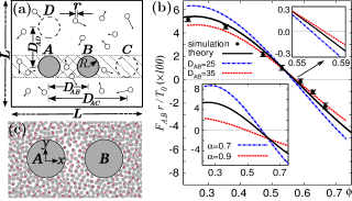
Figure 1: (color online) (a) Sketch of the simulation cell. (b) $F_{{}_{\text{A,B}}}$ scaled by $T_{{}_{0}}/r$ vs $\phi$. Comparison is made with the solution of Eq. (2) for the reference system (solid line), as well as other values of the control parameters $D\!_{{}_{\text{AB}}}$ and $\alpha$ (dashed lines). (c) Typical snapshots of dense (gray circles) and dilute (red crosses) states with $\phi{=}0.66$ and $0.24$, respectively.

In the present Letter, we study the effective interactions between immobile intruder particles immersed in a uniformly agitated granular fluid where all particles undergo inelastic binary collisions (Fig. 1). We show that the interaction between a pair of intruders exhibits a crossover from attraction to repulsion below a critical density, as predicted in 12 . We here address the general conditions under which the transition happens, and present the phase diagram of the transition. Moreover, by comparing the behavior of two and multi intruder systems, we find that the fluctuation-induced force is not derived from a pair-potential; inserting a new intruder affects the previously existing interactions in a non-trivial way, depending on the relative positions of the intruders. Such a feature together with the possible sign change of the forces make the multi-body interactions more complicated and may lead to a variety of collective behaviors such as segregation, clustering, or pattern formation. Analytical calculations using the theory of randomly driven granular fluids 15 confirm our findings.

Simulation method — We consider a 2D granular fluid similar to the setup described in Refs.16 ; 15 ; 12 by means of molecular dynamics simulations. We have a reference system with two intruders A and B in which $L_{{}_{0}}/r{=}200$, $R_{{}_{0}}/r{=}10$, and $D\!_{{}_{\text{AB},0}}/r{=}30$ [see Fig. 1(a)]. The reference volume fraction $\phi_{{}_{0}}$ is $0.66$, and the normal restitution coefficient $\alpha_{{}_{0}}$ is set to 0.8 for all collisions. Periodic boundary conditions are applied in both directions of the square-shaped cell to provide a spatially homogeneous state. The system is coupled to an external heat bath that uniformly transfers energy into the system; the acceleration of each particle $\bm{a}_{i}$ is perturbed instantaneously by a random amount $\bm{\xi}_{i}$ which can be considered as a Gaussian white noise with zero mean and correlation $\langle\xi_{ia}(t)\xi_{jb}(t^{\prime})\rangle{=}\xi^{2}\delta_{ij}\delta_{ab}\delta(t-t^{\prime})$, where $a$ and $b$ denote Cartesian components of the vectors, and $\xi$ is the driving strength. The rate of the energy gain of a single particle averaged over the uncorrelated noise source is $\partial_{t}E{=}m\xi^{2}$ 15 . Each particle also loses energy due to inelastic collisions at the mean-field rate of $\partial_{t}E{=}(\alpha^{2}\!-\!1)\omega T/2$ 18 ; 17 , where $T$ is the granular temperature and $\omega$ is the collision frequency given by the Enskog theory 19 . Eventually, the system reaches a nonequilibrium stationary state by balancing the energy input and the dissipation.

Figure 2: (a) $F\!\!_{{}_{\text{A,B}}}$ vs $D\!_{{}_{\text{AB}}}$. The solid line is obtained via Eq. (2). (b) $F\!\!_{{}_{\text{A,B}}}$ vs $T$. The dashed line indicates a linear relation. Values of $F$ around $10^{-3}T\!_{{}_{0}}/r$ reflect the accuracy level of our calculation. (c) $F\!\!_{{}_{\text{A,B}}}$ vs $L$. The dashed line corresponds to ${h}(L)$. The inset shows that the deviation of the results from ${h}(L)$ has no systematic dependence on $L$. $\phi{=}0.24$ in all cases.

Effective two-body interactions — In the steady state we measure the total force exerted by the granular fluid on each intruder along the $x$ axis during the time interval $\tau$ ($\tau\!\!\sim\!\!250$ collisions per particle). Due to the observed large fluctuations, the force is measured for more than $10^{4}$ consecutive time intervals $\tau$. The probability distribution of the data is well fitted by a Gaussian 20 with the standard deviation $\sigma{=}0.244T\!_{{}_{0}}/r$ and the nonzero mean $F_{{}_{0}}{=}-0.023T\!_{{}_{0}}/r$, where $T\!_{{}_{0}}$ is the mean-field approximation of the steady-state temperature deduced from the Enskog theory 15 . Using a similar analysis along the $y$ axis, we obtain zero force within the accuracy of our measurements. $F_{{}_{0}}$ can be considered as the magnitude of the effective force $F\!\!_{{}_{\text{A,B}}}$ that the intruder B exerts on A, which is attractive in this case. We observe that, upon decreasing the volume fraction below a critical value $\phi_{{}_{c}}\!\!\sim\!\!0.57$, the effective interaction $F\!\!_{{}_{\text{A,B}}}$ becomes repulsive [Fig. 1(b)], in agreement with the prediction of Ref. 12 . However, the transition is controlled not only by $\phi$, but also by $D\!_{{}_{\text{AB}}}$ and $\alpha$. One expects that, far from the transition region, increasing $D\!_{{}_{\text{AB}}}$ decreases the magnitude of $F\!\!_{{}_{\text{A,B}}}$ and it should eventually vanish at $D\!_{{}_{\text{AB}}}{=}L/2$ due to periodic boundary conditions, as confirmed by simulations [Fig. 2(a)]. In Fig. 2(b), by varying the driving strength $\xi$, it is shown that $F$ is proportional to the steady state temperature. Moreover, the results reveal the impact of dimensionality on the process: $F$ increases slightly with $L$ when we vary the system size while other parameter values are kept fixed. The simulation results, shown in Fig. 2(c), can be well fitted by a logarithmic growth $h(L){=}a\ln(L){+}b$ (dashed line). This is contrary to what happens in three dimensional systems, where the force is independent of $L$.

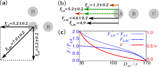
Figure 3: (color online) Comparison between the binary and triple effective forces (scaled by $0.01T\!_{{}_{0}}/r$) exerted on particle A in the presence of particles (a) B and D (b) B and C. (c) $e$, $F\!\!_{{}_{\text{A,BC}}}$ and $F\!\!_{{}_{\text{A,B}}}\!\!+\!F\!\!_{{}_{\text{A,C}}}$ versus $D\!_{{}_{\text{AC}}}$, the $x$ position of particle C.

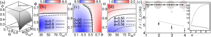
Figure 4: (color online) (a) Schematic phase diagram of the transition in the ($\phi$, $D_{\text{AB}}$, $\alpha$) space. The surface corresponds to $F\!\!_{{}_{\text{A,B}}}{=}0$. (b-d) 2D profiles of the phase diagram where the solid lines mark the interface position. The dashed lines correspond to the interface position for other values of the third control parameter. The color intensity reflects the magnitude of $F$ (scaled by $0.01T\!_{{}_{0}}/r$), with blue (red) meaning repulsion (attraction). (e) $F$ on particle A vs $n$, the length of the chain. The results of the mode coupling, simulation, and pairwise summation of two-body forces are shown with solid line, full circles, and open circles, respectively. Inset: Mode coupling results (solid line) and their corresponding pairwise summations (dashed line) ($L{=}500r$).

Triple configurations and nonadditivity — Next we address the interesting case of triple systems, where the third intruder is located either on the $x$ or $y$ axis (Fig. 3). By choosing $D\!_{{}_{\text{AD}}}\!/\!r{=}30$ and $\phi{=}0.24$, the effective force $\bm{F}\!\!_{{}_{\text{A,BD}}}$ exerted on particle A in the triple configuration (A,B,D) is compared to $\bm{F}\!\!_{{}_{\text{A,B}}}$ and $\bm{F}\!\!_{{}_{\text{A,D}}}$ obtained from the binary systems (A,B) and (A,D), respectively. Note that the simulation is performed anew for each set of intruders. Figure 3(a) shows that $\bm{F}\!\!_{{}_{\text{A,BD}}}$ is nearly the vector sum of $\bm{F}\!\!_{{}_{\text{A,B}}}$ and $\bm{F}\!\!_{{}_{\text{A,D}}}$. However, a comparison between the sets (A,B,C), (A,B), and (A,C) in Figure 3(b) (with $D\!_{{}_{\text{AC}}}\!/\!r{=}70$) reveals that the force is definitely not pairwise additive in this case; $F\!\!_{{}_{\text{A,BC}}}$ is even smaller than $F\!\!_{{}_{\text{A,B}}}$.

In order to understand the mechanism behind the long-range interactions and the transition, we draw attention to the fact that the fluctuating hydrodynamic fields, e.g. density [see Fig. 1(c)], are notably influenced by the geometric constraints, resulting in pressure imbalance around the intruders and effective interactions between them. To establish a quantitative connection between the effective force and the hydrodynamic fluctuations, we first employ mode coupling calculations 15 ; 21 ; 12 to evaluate the two-body interactions. In the nonequilibrium steady state, the hydrodynamic fields ($p(\bm{r})$,$T(\bm{r})$,$n(\bm{r})$) fluctuate around their stationary values ($p_{s}$,$T\!_{s},n_{s}$). The average pressure fluctuation $p_{{}_{f}}\!(\bm{r})$ in the presence of the boundary conditions imposed by intruders behaves analogously to the Casimir effect, i.e., $p_{{}_{f}}\!(\bm{r})$ in the hatched region of Fig. 1(a) differs from that of the cross-hatched region. Using the Verlet-Levesque equation of state for a hard disks system $p(n,T){=}Tf(n)$ (with $f(n){=}n(1+\phi^{2}/8)\!/\!(1-\phi)^{2}$, and $n$ the number density) 22 , we expand the pressure up to second order around ($n_{s},T\!_{s}$), and take the statistical average over the random noise source: $p_{{}_{f}}(\bm{r}){=}f^{\prime}(n)|_{{}_{n\!_{s}}}\langle\delta n(\bm{r})\delta T(\bm{r})\rangle\!+\!\frac{1}{2}T\!_{s}f^{\prime\prime}(n)|_{{}_{n\!_{s}}}\langle(\delta n(\bm{r}))^{2}\rangle$. By Fourier transforming $\delta n(\bm{r})$ and $\delta T(\bm{r})$ one obtains

$$p_{{}_{f}}\!(\bm{r}){=}\int\!\!\left[f^{\prime}(n)|_{{}_{n\!_{s}}}S_{\text{nT}}(\bm{k})\!+\!\frac{1}{2}T\!_{s}f^{\prime\prime}(n)|_{{}_{n\!_{s}}}S_{\text{nn}}(\bm{k})\right]d\bm{k},$$ (1)

where the integral is taken over the $\bm{k}$ vectors allowed at position $\bm{r}$ by the boundary conditions, and $S_{\text{ab}}(\bm{k})$ is the pair structure factor defined as $V^{-1}\langle\delta a(\bm{k})\delta b(-\bm{k})\rangle$. The detailed description of the structure factor calculations will be reported elsewhere (see also Ref. 15 ). Here we denote the integrand of Eq. (1) with $g(\bm{k},\phi,\alpha)$ and compare $p_{{}_{f}}\!(\bm{r})$ for two surface points located on opposite sides of intruder A with the same $y$ coordinates. The related $\bm{k}$ vectors in the $x$ direction are confined to $D\!_{{}_{\text{in}}}\!(y){=}D\!_{{}_{\text{AB}}}\!\!-\!2\sqrt{(}R^{2}\!\!-\!\!y^{2})$ and $D\!_{{}_{\text{out}}}\!(y){=}L\!-\!D\!_{{}_{\text{AB}}}\!\!\!-\!\!2\sqrt{(}R^{2}\!\!-\!\!y^{2})$ in the cross-hatched and hatched regions, respectively; Therefore the pressure difference between these two points $\Delta p(y){=}p^{\text{(in)}}_{{}_{f}}\!-\!p^{\text{(out)}}_{{}_{f}}$ has $y$ dependence. By integrating over $y$, we arrive at the average pressure difference between the gap and outside region:

$$\Delta p{=}\!\!\!\int_{-R}^{R}\!\!\!\!\!dy\!\!\left[\!\int_{2\pi\!/\!D\!_{{}_{\text{in}}}\!\!(y)}^{2\pi\!/\!r^{*}}\!\!\!\!\!\!\!\!\!\!\!dk_{{}_{x}}\!\!\!-\!\!\!\int_{2\pi\!/\!D\!_{{}_{\text{out}}}\!(y)}^{2\pi\!/\!r^{*}}\!\!\!\!\!\!\!\!\!dk_{{}_{x}}\right]\!\!\int_{2\pi\!/\!L}^{2\pi\!/\!r^{*}}\!\!\!\!\!\!\!dk_{{}_{y}}\!\!\frac{g(k_{x},k_{y},\phi,\alpha)}{2R}.$$ (2)

To ensure that the hydrodynamic description is valid, the integrals are restricted to the long wavelength range $r^{*}{=}\text{max}(2r,l^{*})$ (with $l^{*}$ being the mean free path) and only small inelasticities are considered. Moreover, $D\!_{{}_{\text{AB}}}$ is always chosen large enough ($3R{\leq}D\!_{{}_{\text{AB}}}$) so that the short-range depletion forces 23 do not play a role. The effective force $F\!_{{}_{\text{AB}}}\!$ is calculated via Eq. (2) for different values of $\phi$ or $D\!_{{}_{\text{AB}}}$ and compared to the simulation results in Figs. 1(b) and 2(a). The forces are of the same order of magnitude as those obtained from the simulations. The deviations can be attributed to the fact that the hydrodynamic fluctuations are correlated in the gap and outside regions. The correction due to this effect is proportional to $\partial^{2}g/\partial\phi^{2}$ which always has a sign opposite to that of $g$, thus, Eq. (2) overestimates the magnitude of the force. Using the mode coupling calculations, it is shown in Fig. 1(b) that the transition point is sensitive to the choice of $D\!_{{}_{\text{AB}}}$ and $\alpha$. The set of control parameters for sign switching of the Casimir force crucially depends on the physics of the system (see e.g. 24 ). Figure 4 summarizes the calculations in a phase diagram in the ($\phi$, $\alpha$, $D\!_{{}_{\text{AB}}}$) space, which appears to be in remarkable accord with the dynamical model. The phase diagram is not influenced by the choice of the steady-state temperature $T\!_{s}$, while the magnitude of the force grows linearly with $T\!_{s}$ as expected for Casimir forces in thermal fluctuating media 14 . Regarding the fact, that the leading term of $g(\bm{k},\phi,\alpha)$ at small $k$ is proportional to $1/k^{2}$ 15 , one also finds from Eq. (1) that $p_{{}_{f}}$, and therefore the force, in the thermodynamic limit behaves as $1/r$ in 3D while diverges logarithmically as $\text{ln}(L/r)$ in 2D.

Multi-body effects — In the triple system of Fig. 3(a), loosely speaking, because of the independence of $k$ vectors in $x$ and $y$ directions one expects that the vector sum holds. This is in agreement with the simulation results in Fig. 3(a), neglecting the deviation due to hydrodynamic correlations. In the configuration of Fig. 3(b), the effective force exerted on particle A results from the difference between the range of available $k$ modes on its left and right sides. In the presence of particle C, the range of allowed $k$ modes decreases on the left side due to periodic boundary conditions, which causes a lowering of pressure difference between both sides of A. The effective force $F\!\!_{{}_{\text{A,BC}}}$ is thus smaller, compared to the binary interaction $F\!\!_{{}_{\text{A,B}}}$. The calculated force on particle A using Eq. (2) is shown with $\widetilde{F}\!\!_{{}_{\text{A,BC}}}$ in Fig. 3(b); the agreement is satisfactory. We introduce a measure $e{=}|\bm{F}\!\!_{{}_{\text{A,B}}}\!\!+\!\!\bm{F}\!\!_{{}_{\text{A,C}}}\!\!-\!\!\bm{F}\!\!_{{}_{\text{A,BC}}}|/|\bm{F}\!\!_{{}_{\text{A,B}}}|$ for quantifying the deviation from the case that the interactions are derived from a pair-potential. Figure 3(c) shows how $e$, obtained from the mode coupling calculations, behaves when the position of particle C is varied on the $x$ axis. Figure 4(e) indicates that our analytical approach also provides reasonable estimates of the effective force acting on particle A in a chain configuration, while the deviation from pairwise summation of two-body forces grows with the number of intruders, $n$.

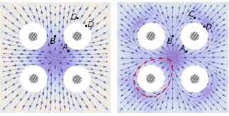
Figure 5: The trajectories of a test intruder subject to the effective force field in a fixed square configuration of intruders, obtained from the mode coupling calculations for $\phi{=}0.24$ (left), and $0.54$ (right). Short range interactions are excluded (white zones). Lighter colors mean stronger forces. The dashed line in the right figure indicates the border of an attractive subdomain, where the trajectories of the test particle end up on the fixed intruder.

Table 1: Comparison between the theoretical (T) and simulation (S) results for the selected points in Figs. 5(left) and 5(right). Same force scales as Fig. 3. The maximum error bars for the simulated $F$ and $\theta$ are $\pm 0.1$ and $\pm 7^{\circ}$, respectively.

	$|\vec{F}|_{(A)}$	$|\vec{F}|_{(B)}$	$|\vec{F}|_{(C)}$	$|\vec{F}|_{(D)}$	$\theta_{(A)}$	$\theta_{(B)}$	$\theta_{(C)}$	$\theta_{(D)}$
left-S	$1.0$	$2.2$	$3.4$	$3.7$	$13^{\circ}$	$92^{\circ}$	$51^{\circ}$	$44^{\circ}$
left-T	$1.17$	$2.52$	$3.97$	$4.32$	$7^{\circ}$	$90^{\circ}$	$60^{\circ}$	$45^{\circ}$
right-S	$0.2$	$0.2$	$0.2$	$0.0$	$19^{\circ}$	$88^{\circ}$	$-32^{\circ}$	$-$
right-T	$0.24$	$0.26$	$0.25$	$0.02$	$28^{\circ}$	$90^{\circ}$	$-24^{\circ}$	$225^{\circ}$

Finally, we investigate more complicated geometries by calculating the effective force field of a fixed square structure acting on a test intruder particle. To elucidate the impact of sign switching on the force pattern we compare an intermediate density (around the transition zone) with a low density case. Figure 5 shows that the patterns are clearly different e.g. in terms of the number of equilibrium points. There exist also attractive subdomains of length scale $\ell$ around the fixed intruders in the right figure (e.g. the domain surrounded by the dashed line). Depending on the choice of control parameters, $\ell$ ranges between $0$ (entirely repulsive patterns at low densities, as shown in the left figure) and $L$ (entirely attractive patterns at high densities, not shown) leading to different types of collective behavior such as segregation, clustering, and pattern formation. Putting aside the pairwise summations, we compare the mode coupling predictions with simulation results at four selected points in Fig 5. The predicted forces are of the same order of magnitude as the simulation results (see table 1), however, the errors of the force size $|F|$ and its direction $\theta$ reach up to $30\%$ and $15^{\circ}$, respectively. The differences are smaller at large distances and also low densities. Indeed, the hydrodynamic correlations become more important in multi-body cases and, hence, one should include triplet or higher order structure factors 25 in mode coupling calculations to properly take the multi-body effects into account.

In conclusion, we focus on the problem of long-range fluctuation-induced forces between intruder particles immersed in an agitated fluid bed. The sign of the force can be reversed by tuning the control parameters. Furthermore, the multi-body interactions do not follow from two-body force descriptions. A newly inserted intruder, depending on its position, may affect the pressure balance around the other intruders. This suggests that the effective force is not derived from a pair-potential in agreement with our simulation results. Our findings represent a step forward in understanding the origin of collective behaviors in fluidized granular mixtures.

We would like to thank I. Goldhirsch for helpful discussions and J. Török and B. Farnudi for comments on the manuscript. Computing time was provided by John-von-Neumann Institute of Computing (NIC) in Jülich.

References

- (1) H. M. Jaeger, S. R. Nagel, and R. P. Behringer, Rev. Mod. Phys. 68, 1259 (1996).
- (2) A. Kudrolli, Rep. Prog. Phys. 67, 209 (2004).
- (3) O. Pouliquen, J. Delour, and S. B. Savage, Nature 386, 816 (1997); L. Hsu, W. E. Dietrich, and L. S. Sklar, J. Geophys. Res. 113, F02001 (2008).
- (4) J. C. Williams, Powder Technol. 15, 245 (1976); J. M. Ottino and D. V. Khakhar, Annu. Rev. Fluid Mech. 32, 55 (2000).
- (5) M. P. Ciamarra, M. D. De Vizia, A. Fierro, M. Tarzia, A. Coniglio, and M. Nicodemi, Phys. Rev. Lett. 96, 058001 (2006).
- (6) D. C. Hong, P. V. Quinn, and S. Luding, Phys. Rev. Lett. 86, 3423 (2001); M. Tarzia, A. Fierro, M. Nicodemi, and A. Coniglio, Phys. Rev. Lett. 93, 198002 (2004); M. Tarzia, A. Fierro, M. Nicodemi, M. P. Ciamarra, and A. Coniglio, Phys. Rev. Lett. 95, 078001 (2005); K. M. Hill and Y. Fan, Phys. Rev. Lett. 101, 088001 (2008).
- (7) T. Shinbrot, Nature 429, 352 (2004).
- (8) D. A. Sanders, M. R. Swift, R. M. Bowley, and P. J. King, Phys. Rev. Lett. 93, 208002 (2004).
- (9) M. P. Ciamarra, A. Coniglio, and M. Nicodemi, Phys. Rev. Lett. 97, 038001 (2006); I. Zuriguel, J. F. Boudet, Y. Amarouchene, and H. Kellay, Phys. Rev. Lett. 95, 258002 (2005).
- (10) T. Schnautz, R. Brito, C. A. Kruelle, and I. Rehberg, Phys. Rev. Lett. 95, 028001 (2005).
- (11) E. Caglioti, A. Coniglio, H. J. Herrmann, V. Loreto, and M. Nicodemi, Europhys. Lett. 43, 591 (1998); T. Shinbrot and F. J. Muzzio, Phys. Rev. Lett. 81, 4365 (1998); T. Mullin, Phys. Rev. Lett. 84, 4741 (2000); G. Metcalfe, S. G. K. Tennakoon, L. Kondic, D. G. Schaeffer, and R. P. Behringer, Phys. Rev. E 65, 031302 (2002).
- (12) C. Cattuto, R. Brito, U. M. B. Marconi, F. Nori, and R. Soto, Phys. Rev. Lett. 96, 178001 (2006).
- (13) S. Aumaitre, C. A. Kruelle, and I. Rehberg, Phys. Rev. E 64, 041305 (2001).
- (14) M. Kardar and R. Golestanian, Rev. Mod. Phys. 71, 1233 (1999).
- (15) T. P. C. van Noije, M. H. Ernst, E. Trizac, and I. Pagonabarraga, Phys. Rev. E 59, 4326 (1999).
- (16) G. Peng and T. Ohta, Phys. Rev. E 58, 4737 (1998).
- (17) I. Goldhirsch and G. Zanetti, Phys. Rev. Lett. 70, 1619 (1993).
- (18) T. P. C. van Noije, M. H. Ernst, and R. Brito, Phys. Rev. E 57, R4891 (1998).
- (19) S. Chapman and T. G. Cowling, The Mathematical Theory of Non-uniform Gases (Cambridge University Press, Cambridge, 1970).
- (20) D. Bartolo, A. Ajdari, J. B. Fournier, and R. Golestanian, Phys. Rev. Lett. 89, 230601 (2002).
- (21) R. Brito and M. H. Ernst, Europhys. Lett. 43, 497 (1998).
- (22) L. Verlet and D. Levesque, Mol. Phys. 46, 969 (1982).
- (23) R. Roth, R. Evans, and S. Dietrich, Phys. Rev. E 62, 5360 (2000); C. N. Likos, Phys. Rep. 348, 267 (2001).
- (24) C. Hertlein, L. Helden, A. Gambassi, S. Dietrich, and C. Bechinger, Nature 451, 172 (2008); M. Levin, A. P. McCauley, A. W. Rodriguez, M. T. Homer Reid, and S. G. Johnson, Phys. Rev. Lett. 105, 090403 (2010).
- (25) P. Attard, J. Chem. Phys. 91, 3072 (1989); S. Jorge, E. Lomba, and J. L. F. Abascal, J. Chem. Phys. 116, 730 (2002).