Magnetic order in quasi–two-dimensional molecular magnets
investigated with muon-spin relaxation

Abstract

We present the results of a muon-spin relaxation (µ${}^{\text{+}}$SR) investigation into magnetic ordering in several families of layered quasi–two-dimensional molecular antiferromagnets based on transition metal ions such as $S=\frac{1}{2}$ Cu${}^{\text{2+}}$ bridged with organic ligands such as pyrazine. In many of these materials magnetic ordering is difficult to detect with conventional magnetic probes. In contrast, µ${}^{\text{+}}$SR allows us to identify ordering temperatures and study the critical behavior close to $T_{\mathrm{N}}$. Combining this with measurements of in-plane magnetic exchange $J$ and predictions from quantum Monte Carlo simulations we may assess the degree of isolation of the 2D layers through estimates of the effective inter-layer exchange coupling and in-layer correlation lengths at $T_{\mathrm{N}}$. We also identify the likely metal-ion moment sizes and muon stopping sites in these materials, based on probabilistic analysis of the magnetic structures and of muon–fluorine dipole–dipole coupling in fluorinated materials.

I Introduction

The $S=\frac{1}{2}$ two-dimensional square-lattice quantum Heisenberg antiferromagnet (2DSLQHA) continues to be one of the most important theoretical models in condensed matter physics Manousakis1991-2DSLHAFM . Experimental realizations of the 2DSLQHA in crystals also contain an interaction between planes, so that the relevant model describing the coupling of electronic spins $\bm{S}_{i}$ gives rise to the Hamiltonian

$$\mathcal{H}=J\sum_{\langle i,j\rangle_{xy}}\bm{S}_{i}\cdot\bm{S}_{j}+J_{\perp}\sum_{\langle i,j\rangle_{z}}\bm{S}_{i}\cdot\bm{S}_{j},$$ (1)

where $J$ ($J_{\perp}$) is the strength of the in- (inter-) plane coupling and the first (second) summation is over neighbors parallel (perpendicular) to the 2D $xy$-plane. Any 2D model ($J_{\perp}=0$) with continuous symmetry will not show long-range magnetic order (LRO) for $T>0$ due to a divergence of infrared fluctuations Mermin1966-and-Wagner-no-1-2D-order ; Berezinskii1971-Mermin-and-Wagner . However, layered systems approximating 2D models ($J_{\perp}\neq 0$) will inevitably enjoy some degree of interlayer coupling and this will lead to magnetic order, albeit at a reduced temperature due to the influence of quantum fluctuations. Quantum fluctuations are also predicted to reduce the value of the magnetic moment in the ground state of the 2DSLQHA to around 60% of its classical value Manousakis1991-2DSLHAFM , and this reduction is often seen in the ordered moments of real materials. In layered materials that approximate the 2DSLQHA, the measurement of the antiferromagnetic ordering temperature $T_{\mathrm{N}}$ is often problematic due not only to this reduction of the magnetic moment, but also to short-range correlations that build up in the quasi-2D layers above $T_{\mathrm{N}}$. These correlations lead to a reduction in the size of the entropy change that accompanies the phase transition, reducing the size of the anomaly in the measured specific heat sengupta2003-bulkmeasuresbad . We have shown in a number of previous cases that muon-spin relaxation (µ${}^{\text{+}}$SR) measurements do not suffer from these effects and therefore represent an effective method for detecting magnetic order in complex anisotropic systems Blundell2007-muSR-lowD-magnets-review ; goddard2008-2DHMexchange ; lancaster2007-CuPz2ClO42 ; lancaster2006-CuPzN .

The rich chemistry of molecular materials allows for the design and synthesis of a wide variety of highly-tunable magnetic model systems Blundell2004-molmagreview . Magnetic centers, exchange paths and the surrounding molecular groups can all be systematically modified, allowing investigation of their effects on magnetic behavior. In particular, the existence of different exchange paths along different spatial directions can result in quasi–low-dimensional magnetic behavior (i.e. systems with magnetic interactions constrained to act in a two-dimensional plane or along a one-dimensional chain). Such systems have the potential to better approximate low-dimensional models than many traditional inorganic materials. In addition, these molecular materials can have exchange energy scales of order $J/k_{\mathrm{B}}\sim 10\mathrm{\;K}$ which are accessible with typical laboratory magnetic fields goddard2008-2DHMexchange of $B\sim 10\mathrm{\;T}$ allowing an additional avenue for their experimental study. This contrasts with typical inorganic low-dimensional systems where the exchange is found to be $J/k_{\mathrm{B}}\sim 1000\mathrm{\;K}$ and fields of $B\sim 1000\mathrm{\;T}$ would be needed to significantly perturb the spin system.

It has also been shown Xiao2009-XY-q2DHA ; Sengupta2009-nonmonotonic-TN-B-CuHF2pyz2BF4 that a small $XY$-like anisotropy exists in some molecular materials. Although $J_{\perp}$ is the decisive energy scale for the magnetic ordering, this anisotropy has been shown to have an influence on the ordering temperature Xiao2009-XY-q2DHA and determines the shape of the low-field $B$–$T$ phase diagram of these systems Sengupta2009-nonmonotonic-TN-B-CuHF2pyz2BF4 .

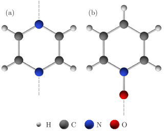
Figure 1: Bridging ligands used in the compounds described in this paper: (a) pyrazine (N${}_{\text{2}}$C${}_{\text{4}}$H${}_{\text{4}}$, abbreviated pyz); and (b) (ii) pyridine-N-oxide (C${}_{\text{5}}$H${}_{\text{5}}$NO, abbreviated pyo). Dashed lines indicate where the ligands bond to other parts of molecular structures.

Several classes of molecular magnetic material closely approximate the 2DSLQHA model and in this paper we report the results of µ${}^{\text{+}}$SR measurements performed on several such materials. These systems are self-assembled coordination polymers, based around paramagnetic ions such as Cu${}^{\text{2+}}$, linked by neutral bridging ligands and coordinating anion molecules. Our materials are based on combinations of three different ligands: (i) pyrazine (N${}_{\text{2}}$C${}_{\text{4}}$H${}_{\text{4}}$, abbreviated pyz) and (ii) pyridine-N-oxide (C${}_{\text{5}}$H${}_{\text{5}}$NO, abbreviated pyo), both of which are planar rings; and (iii) the linear bifluoride ion [(HF${}_{\text{2}}$)^-], which is bound by strong hydrogen bonds F${}^{\text{...}}$H${}^{\text{...}}$F. The pyz and pyo ligands are shown in Fig. 1. Specifically, we investigate the molecular system [M(HF${}_{\text{2}}$)(pyz)${}_{\text{2}}$]X, where M${}^{\text{2+}}$ = Cu${}^{\text{2+}}$ is the transition metal cation and X^- is one of various anions (e.g. BF${}_{\text{4}}^{-}$, ClO${}_{\text{4}}^{-}$, PF${}_{\text{6}}^{-}$ etc.). We also report the results of our measurements on other quasi-2D systems. First, [Cu(pyz)${}_{\text{2}}$(pyo)${}_{\text{2}}$]Y${}_{\text{2}}$, with Y^- = BF${}_{\text{4}}^{-}$ or PF${}_{\text{6}}^{-}$, in which pyo ligands bridge Cu(pyz)${}_{\text{2}}$ planes. Then, the quasi-2D non-polymeric compounds [Cu(pyo)${}_{\text{6}}$]Z${}_{\text{2}}$, where Z^-=BF${}_{\text{4}}^{-}$, ClO${}_{\text{3}}^{-}$ or PF${}_{\text{6}}^{-}$ are examined. We also investigate materials in which either Ni${}^{\text{2+}}$ ($S=1$) or Ag${}^{\text{2+}}$ ($S=\frac{1}{2}$) form the magnetic species in the quasi-2D planes rather than Cu${}^{\text{2+}}$.

This paper is structured as follows. In Sec. II we outline the µ${}^{\text{+}}$SR technique and describe our experimental methods. The [Cu(HF${}_{\text{2}}$)(pyz)${}_{\text{2}}$]X family of materials is then discussed in Sec. III, where muon data are used to determine $T_{\mathrm{N}}$ and critical parameters. Muon–fluorine dipole–dipole oscillations in the paramagnetic regime are found for these materials which we use, in conjunction with dipole field simulations, to investigate possible muon sites and constrain the copper moment. In Sec. IV we explore the related 2D system [Cu(pyz)${}_{\text{2}}$(pyo)${}_{\text{2}}$]Y${}_{\text{2}}$. Sec. V details measurements of [Cu(pyo)${}_{\text{6}}$]Z${}_{\text{2}}$. Sec. VI examines a highly two-dimensional silver-based molecular material, Ag(pyz)${}_{\text{2}}$(S${}_{\text{2}}$O${}_{\text{8}}$). Finally, data from the [Ni(HF${}_{\text{2}}$)(pyz)${}_{\text{2}}$]X (X^- = PF${}_{\text{6}}^{-}$, SbF${}_{\text{6}}^{-}$) family of molecular magnets is presented in Sec. VII.

II Experimental details

Zero-field (ZF) µ${}^{\text{+}}$SR measurements were made on powder samples of the materials at the ISIS facility, Rutherford Appleton Laboratory, UK using the MuSR and EMU instruments and the Swiss Muon Source (SµS), Paul Scherrer Institut, Switzerland using the General-Purpose Surface-Muon (GPS) instrument and Low-Temperature Facility (LTF). For measurements at temperatures $T\geq 1.8\mathrm{\;K}$ powder samples were packed in a $25\mathrm{\;\mathchoice{\hbox{\normalsize\textmu}}{\hbox{\normalsize\textmu}}{\hbox{\scriptsize\textmu}}{\hbox{\tiny\textmu}}m}$ Ag foil packet and mounted on a Ag backing plate. For measurements at $T<1.8\mathrm{\;K}$ the samples were mounted directly on an Ag plate and covered with a $12.5\mathrm{\;\mathchoice{\hbox{\normalsize\textmu}}{\hbox{\normalsize\textmu}}{\hbox{\scriptsize\textmu}}{\hbox{\tiny\textmu}}m}$ Ag foil mask. Ag is used since it has only a small nuclear magnetic moment, and so minimizes the background depolarization of the muon spin ensemble.

In a µ${}^{\text{+}}$SR experiment blundell1999-mureview , spin-polarized positive muons are stopped in a target sample. The positive muons are attracted to areas of negative charge density and often stop at interstitial positions. The observed property of the experiment is the time evolution of the muon-spin polarization, the behaviour of which depends on the local magnetic field at the muon site. Each muon decays with an average lifetime of $2.2\mathrm{\;\mathchoice{\hbox{\normalsize\textmu}}{\hbox{\normalsize\textmu}}{\hbox{\scriptsize\textmu}}{\hbox{\tiny\textmu}}s}$ into two neutrinos and a positron, the latter particle being emitted preferentially along the instantaneous direction of the muon spin. Recording the time dependence of the positron emission directions therefore allows the determination of the spin polarization of the ensemble of muons. In our experiments, positrons are detected by detectors placed forward ($\mathrm{F}$) and backward ($\mathrm{B}$) of the initial muon polarization direction. Histograms $N_{\mathrm{F}}(t)$ and $N_{\mathrm{B}}(t)$ record the number of positrons detected in the two detectors as a function of time following the muon implantation. The quantity of interest is the decay positron asymmetry function, defined as

$$A(t)=\frac{N_{\mathrm{F}}(t)-\alpha N_{\mathrm{B}}(t)}{N_{\mathrm{F}}(t)+\alpha N_{\mathrm{B}}(t)}\,,$$ (2)

where $\alpha$ is an experimental calibration constant. The asymmetry, $A(t)$, is proportional to the spin polarization of the muon ensemble.

A muon spin will precess around the local magnetic fields at its stopping site at a frequency $\nu=\gamma_{\mathchoice{\hbox{\normalsize\textmu}}{\hbox{\normalsize\textmu}}{\hbox{\scriptsize\textmu}}{\hbox{\tiny\textmu}}}B/2\pi$, where the muon gyromagnetic ratio $\gamma_{\mathchoice{\hbox{\normalsize\textmu}}{\hbox{\normalsize\textmu}}{\hbox{\scriptsize\textmu}}{\hbox{\tiny\textmu}}}=2\pi\times 135.5\mathrm{\;MHz\,T^{-1}}$. In the presence of LRO in a material we often measure oscillations in $A(t)$. These result from a significant number of muons stopping at sites with a similar internal field, giving rise to a coherent precession of the ensemble of muon spins. Since the spins precess in local magnetic fields directed perpendicularly to the spin polarization direction, we would expect that, for a powder sample with a static magnetic field distribution, $\frac{2}{3}$ of the total spin components should precess and the remaining $\frac{1}{3}$ should be non-relaxing. The non-relaxing third of muon-spin components give rise to the so-called $\frac{1}{3}$-tail in $A(t)$, whose presence therefore provides additional evidence for a static field distribution in powder sample. Taken together, these effects provide an unambiguous method for sensitively identifying a transition to LRO. An example of typical spectra above and below the magnetic ordering temperature is shown for [Cu(HF${}_{\text{2}}$)(pyz)${}_{\text{2}}$]BF${}_{\text{4}}$ in Fig. 2; the oscillations above $T_{\mathrm{N}}$ are characteristic of a quantum-entangled Fµ  state (see Sec. III.4).

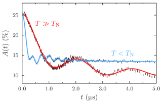
Figure 2: Example $A(t)$ spectra with fits above ($T=25$ K) and below ($T=0.35$ K) the magnetic transition temperature $T_{\mathrm{N}}=1.4$ K for [Cu(HF${}_{\text{2}}$)(pyz)${}_{\text{2}}$]BF${}_{\text{4}}$. Note the approximately equal initial asymmetry, and the oscillations and ‘$\frac{1}{3}$-tail’ observed in the ordered phase. The slow oscillation observed for $T>T_{\mathrm{N}}$ is due to muon–fluorine dipole–dipole oscillations.

III $\text{[Cu(HF}_{\text{2}}\text{)(pyz)}_{\text{2}}\text{]}\text{\emph{X}}$

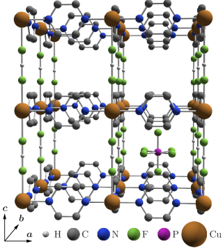
Figure 3: The structure of [Cu(HF${}_{\text{2}}$)(pyz)${}_{\text{2}}$]PF${}_{\text{6}}$, as an example of the [M(HF${}_{\text{2}}$)(pyz)${}_{\text{2}}$]X series. Copper ions are joined in a 2D square lattice by pyrazine ligands to form Cu(pyz)${}_{\text{2}}^{\text{2+}}$ sheets; the 2D layers are joined in the third dimension by HF${}_{\text{2}}^{-}$ groups, making a pseudocubic 3D structure; and this structure is stabilised by a PF${}_{\text{6}}^{-}$ anion at the center of each cubic pore. For clarity, hydrogen atoms attached to pyrazine rings have been omitted, and only one PF${}_{\text{6}}^{-}$ anion is shown.

The synthesis of the [M(HF${}_{\text{2}}$)(pyz)${}_{\text{2}}$]X system manson2006-CuHF2pyz2BF4-chemcomm ; goddard2008-2DHMexchange ; manson2009-HFsynthons-JACScover represented the first example of the use of a bifluoride building block to make a three-dimensional coordination polymer. This class of materials possesses a highly stable structure due to the exceptional strength of the bifluoride hydrogen bonds. The structure of the [M(HF${}_{\text{2}}$)(pyz)${}_{\text{2}}$]X system manson2006-CuHF2pyz2BF4-chemcomm ; manson2009-HFsynthons-JACScover comprises infinite 2D [M(pyz)${}_{\text{2}}$]${}^{\text{2+}}$ sheets which lie in the $ab$ plane, with bifluoride ions (HF${}_{\text{2}}$)^- above and below the metal ions, acting as bridges between the planes to form a pseudocubic network. The X^- anions occupy the body-center positions within each cubic pore. An example structure, for [Cu(HF${}_{\text{2}}$)(pyz)${}_{\text{2}}$]PF${}_{\text{6}}$, is shown in Fig. 3. Samples are produced in polycrystalline form via aqueous chemical reactions between MX${}_{\text{2}}$ salts and stoichiometric amounts of ligands. Preparation details for the compounds are reported in Refs. manson2006-CuHF2pyz2BF4-chemcomm, ; manson2009-HFsynthons-JACScover, ; Manson2011-NiHF2pyz2X, .

In this section we consider those materials where the M cations are Cu${}^{\text{2+}}$ 3d${}^{\text{9}}$ $S=\frac{1}{2}$ centers. It is thought that the magnetic behavior of these material results from the $3d_{x^{2}-y^{2}}$ orbital of the Cu at the center of each CuN${}_{\text{4}}$F${}_{\text{2}}$ octahedron lying in the CuN${}_{\text{4}}$ plane so that the spin exchange interactions between neighboring Cu${}^{\text{2+}}$ ions occur through the $s$-bonded pyz ligandsmanson2006-CuHF2pyz2BF4-chemcomm . The interplane exchange through the HF${}_{\text{2}}$ bridges connecting two Cu${}^{\text{2+}}$ ions should be very weak as these bridges lie on the 4-fold rotational axis of the Cu $3d_{x^{2}-y^{2}}$ magnetic orbital, resulting in limited overlap with the fluorine $p_{z}$ orbitals. Therefore to a first approximation, the magnetic properties of [M(HF${}_{\text{2}}$)(pyz)${}_{\text{2}}$]X can be described in terms of a 2D square lattice.

Measurements for X^- = BF${}_{\text{4}}^{-}$, ClO${}_{\text{4}}^{-}$ and SbF${}_{\text{6}}^{-}$ were made using the MuSR spectrometer at ISIS, whilst PF${}_{\text{6}}$, AsF${}_{\text{6}}$, NbF${}_{\text{6}}$ and TaF${}_{\text{6}}$ were measured using GPS at PSI.

III.1 Long-range magnetic order

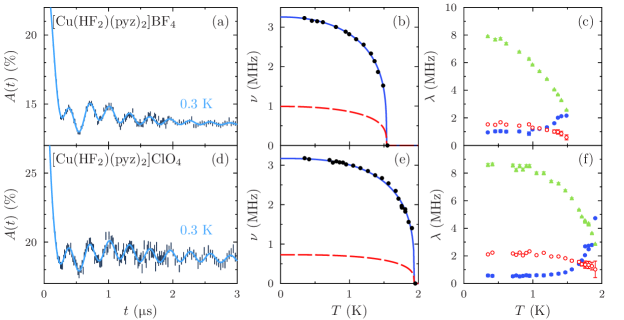
Figure 4: Data and the results of fits to Eq. (3) for [Cu(HF${}_{\text{2}}$)(pyz)${}_{\text{2}}$]X magnets with tetrahedral anions X^-. From left to right: (a) and (d) show sample asymmetry spectra $A(t)$ for $T<T_{\mathrm{N}}$ along with a fit to Eq. (3); (b) and (e) show frequencies as a function of temperature [no data points are shown for the second line because this frequency $\nu_{2}$ was held in fixed proportion to the first, $\nu_{1}$ (see text)]; and (c) and (f) show relaxation rates $\lambda_{i}$ as a function of temperature. In the $\nu(T)$ plot, error bars are included on the points but in most cases they are smaller than the marker being used. The solid line representing $\nu_{1}$ in (b) and (c) corresponds to the filled circles in the third column of graphs [(c) and (f)] for that component’s relaxation, $\lambda_{1}$, whilst the dashed line and unfilled circles correspond to $\nu_{2}$ and $\lambda_{2}$, respectively. The filled triangles correspond to the fast relaxation $\lambda_{3}$.

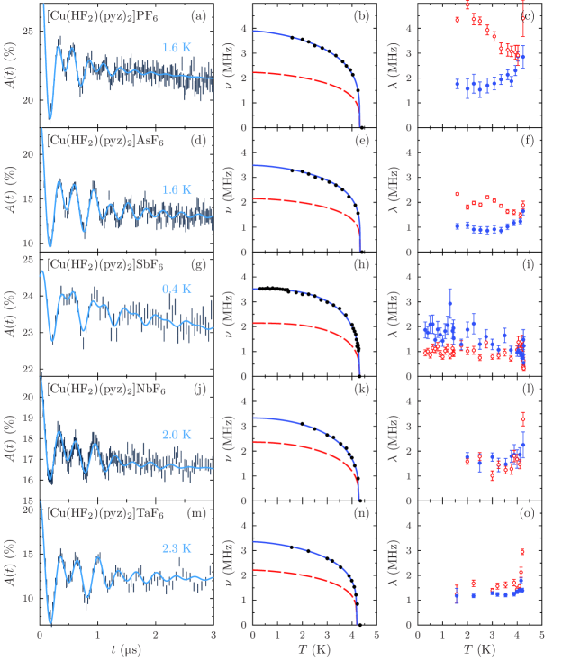
Figure 5: Example data and fits for [Cu(HF₂)(pyz)${}_{\text{2}}$]X magnets with octahedral anions X^-. From left to right: (a), (d), (g), (j) and (m) show sample asymmetry spectra $A(t)$ for $T<T_{\mathrm{N}}$ along with a fit to Eq. (3); (b), (e), (h), (k) and (n) show frequencies as a function of temperature [no data points are shown for the second line because this frequency $\nu_{2}$ was held in fixed proportion to the first, $\nu_{1}$ (see text)]; and (c), (f), (i), (l) and (o) show relaxation rates $\lambda_{i}$ as a function of temperature. In the $\nu(T)$ plot, error bars are included on the points but in most cases they are smaller than the marker being used. The solid line representing $\nu_{1}$ in (b), (e), (h), (k) and (n) corresponds to the filled circles in the third column of graphs [(c), (f), (i), (l) and (o)] for that component’s relaxation, $\lambda_{1}$, whilst the dashed line and unfilled circles correspond to $\nu_{2}$ and $\lambda_{2}$, respectively.

The main result of our measurements on these systems is that below a critical temperature $T_{\mathrm{N}}$, oscillations in the asymmetry spectra $A(t)$ are observed at two distinct frequencies, for all materials in the series. This shows unambiguously that each of these materials undergoes a transition to a state of LRO. Example asymmetry spectra are shown in the left-hand column of Fig. 4 and Fig. 5. They were found to be best fitted with a relaxation function

$$A(t)= A_{0} \left[p_{1}\mathrm{e}^{-\lambda_{1}t}\cos(2\pi\nu_{1}t+\phi_{1})\right.$$ (3)

$$\left.+p_{2}\mathrm{e}^{-\lambda_{2}t}\cos(2\pi P_{2}\nu_{1}t+\phi_{2})+p_{3}\mathrm{e}^{-\lambda_{3}t}\right]$$

$$+A_{\mathrm{bg}}\mathrm{e}^{-\lambda_{\mathrm{bg}}t},$$

where $A_{0}$ represents the contribution from those muons which stop inside the sample and $A_{\mathrm{bg}}$ accounts for a relaxing background signal due to those muons that stop in the silver sample holder or cryostat tails, or with their spin parallel to the local field. Of those muons which stop in the sample, $p_{1}$ indicates the weighting of the component in an oscillating state with frequency $\nu_{1}$; $p_{2}$ is the weighting of a lower-frequency oscillating state with frequency $\nu_{2}$; and $p_{3}$ represents the weighting of a component with a large relaxation rate $\lambda_{3}$. All parameters were initially left free to vary. The second frequency was found to vary with temperature in fixed proportion to $\nu_{1}$ via $\nu_{2}=P_{2}\nu_{1}$ for each material. The parameter $P_{2}$ was identified by fitting the lowest-temperature $A(t)$ spectra where Eq. (3) would be expected to most accurately describe the data, and subsequently held fixed during the fitting procedure. Phase factors $\phi_{i}$ were also found to be necessary in some cases to obtain a reliable fit. The parameters resulting from these fits are listed in Table 1, and data with fits are shown in Figs. 4 and 5. We also note here that the discontinuous nature of the change in all fitted parameters and the form of the spectra at $T_{\mathrm{N}}$ strongly suggest that these materials are magnetically ordered throughout their bulk.

X	$\nu_{1}\mathrm{\>(MHz)}$	$\nu_{2}\mathrm{\>(MHz)}$	$\lambda_{3}\mathrm{\;(MHz)}$	$p_{1}$	$p_{2}$	$p_{3}$	$\phi_{1}\;(^{\circ})$	$\phi_{2}\;(^{\circ})$	$T_{\mathrm{N}}\mathrm{\>(K)}$	$\beta$	$\alpha$	$J/k_{\mathrm{B}}\mathrm{\>(K)}$	$|J_{\perp}/J|$
BF${}_{\text{4}}$	$3.30(6)$	$0.95(3)$	$8$	$15$	$15$	$70$	$-57(1)$	$26(2)$	$1.54(2)$	$0.18(4)$	$1.6(7)$	$6.3$	$9\times 10^{-4}$
ClO${}_{\text{4}}$	$3.2(1)$	$0.64(1)$	$8$	$2$	$2$	$96$	$-94(1)$	$104(4)$	$1.91(1)$	$0.25(2)$	$2.6(3)$	$7.3$	$2\times 10^{-3}$
PF${}_{\text{6}}$	$3.89(6)$	$2.23(5)$	$25$	$30$	$30$	$40$	$-53(3)$	$37(6)$	$4.37(2)$	$0.26(2)$	$1.5(3)$	$12.4$	$1\times 10^{-2}$
AsF${}_{\text{6}}$	$3.49(9)$	$2.15(2)$	$40$	$25$	$25$	$50$	$-14(2)$	$14(3)$	$4.32(3)$	$0.23(3)$	$1.6(5)$	$12.8$	$1\times 10^{-2}$
SbF${}_{\text{6}}$	$3.51(2)$	$2.14(2)$	-	$50$	$50$	-	$-46(3)$	$-20(2)$	$4.29(1)$	$0.34(2)$	$2.8(3)$	$13.3$	$9\times 10^{-3}$
NbF${}_{\text{6}}$	$3.33(7)$	$2.36(5)$	$1$	$40$	$20$	$40$	$0$	$-30(5)$	$4.28(1)$	$0.33(3)$	$2.0(4)$	-	-
TaF${}_{\text{6}}$	$3.33(9)$	$2.21(5)$	-	$50$	$50$	-	$0$	$0$	$4.22(1)$	$0.25(1)$	$1.5(3)$	-	-

Table 1: Fitted parameters for molecular magnets in the [Cu(HF${}_{\text{2}}$)(pyz)${}_{\text{2}}$]X family. The first parameters shown relate to fits to Eq. (3), which allow us to derive frequencies at $T=0$, $\nu_{i}$; probabilities of stopping in the various classes of stopping site, $p_{i}$, in percent; and phases associated with fitting the oscillating components $\phi_{i}$. Then, the temperature dependence of $\nu_{i}$ is fitted with Eq. (4), extracting values for the Néel temperature, $T_{\mathrm{N}}$, critical exponent $\beta$ and parameter $\alpha$. Finally, the quoted $J/k_{\mathrm{B}}$ is obtained from pulsed-field experiments goddard2008-2DHMexchange , and the ratio of inter- to in-plane coupling, $J_{\perp}/J$, is obtained by combining $T_{\mathrm{N}}$ and $J$ with formulae extracted from quantum Monte Carlo simulations (see Sec. III.2, and Ref. goddard2008-2DHMexchange, ). Dashes in the $\lambda_{3}$ column for the SbF${}_{\text{6}}$ and TaF${}_{\text{6}}$ compounds indicate that no fast-relaxing component was used to fit those data. Dashes in the $J/k_{\mathrm{B}}$ and $J_{\perp}/J$ columns for NbF${}_{\text{6}}$ and TaF${}_{\text{6}}$ indicates a lack of pulsed-field data for these materials.

The frequencies and relaxation rates as a function of temperature extracted from these fits are shown in the central column of Figs. 4 and 5. The muon precession frequency, which is proportional to the internal field in the material, can be considered an effective order parameter for the system. Consequently, fitting extracted frequencies as a function of temperature to the phenomenological function

$$\nu(T)=\nu(0)\left[1-\left(\frac{T}{T_{\mathrm{N}}}\right)^{\alpha}\right]^{\beta},$$ (4)

allows an estimate of the critical temperature and the exponent $\beta$ to be extracted. Our results fit well with a previous observation goddard2008-2DHMexchange that the compounds divide naturally into two classes: those with tetrahedral anions X^- = BF${}_{\text{4}}^{-}$, ClO${}_{\text{4}}^{-}$ and those with octahedral anions X^- = AF${}_{\text{6}}^{-}$. The tetrahedral compounds have lower transition temperatures $T_{\mathrm{N}}\lesssim 2\mathrm{\;K}$, as compared to the octahedral compounds’ $T_{\mathrm{N}}\gtrsim 4\;\mathrm{K}$; and the tetrahedral compounds also display slightly lower oscillation frequencies than their octahedral counterparts goddard2008-2DHMexchange .

This difference has been explained  in terms of differences in the crystal structure between the two sets of compounds. Firstly, the octahedral anions are larger than their tetrahedral counterparts. Secondly, the pyrazine rings are tilted by differing amounts with respect to the normal to the 2D layers: those in the octahedral compounds are significantly more upright. Since the Cu $3d_{x^{2}-y^{2}}$ orbitals point along the pyrazine directions, these tilting angles might be expected, to first order, to make little difference to nearest-neighbor exchange because such rotation is about a symmetry axis as viewed from the copper site. However, it may be that the different direction of the delocalized orbitals above and below the rings through which exchange probably occurs, possibly in conjunction with hybridization with the anion orbitals, result in an altered next-nearest neighbor or higher-order interactions, changing the transition temperature.

Within the tetrahedral compounds, the difference in the weighting of the oscillatory component ($p_{1}+p_{2}$) in X^- = BF${}_{\text{4}}^{-}$ and ClO${}_{\text{4}}^{-}$ probably results from the difficulty in fitting the fast-relaxing component. Even with little change in the size of the oscillations, any error assigning the magnitude of this component will affect the proportion of the $A(t)$ signal attributed to them. This difficulty is partly due to the resolution-limited nature of ISIS arising from the pulsed beam structure. In the octahedral compounds, we found that X^- = SbF${}_{\text{6}}^{-}$ and TaF${}_{\text{6}}^{-}$ did not have a resolvable fast-relaxing component, and consequently $p_{3}$ was set to zero during the fitting procedure. This is reflected by dashes in the $p_{3}$ and $\lambda_{3}$ columns in Table 1.

The fact that two oscillatory frequencies are observed points to the existence of at least two magnetically distinct classes of muon site. In general we find that $p_{1}\approx p_{2}$ for these materials, making the probability of occupying the sites giving rise to magnetic precession approximately equal. The weightings $p_{1,2}$ were found to be significantly less than the weighting $p_{3}$ relating to the fast-relaxing site. This, in combination with the magnitude of the fast relaxation $\lambda_{3}(T=0)\gtrsim 10\mathrm{\;MHz}$, suggests that this term should not be identified with the $\frac{1}{3}$-tail which results from muons with spins parallel to their local field. (If that were the case then we would expect $(p_{1}+p_{2})/p_{3}=2$, which we do not observe.) It is likely that each of the components, $p_{1}$, $p_{2}$ and $p_{3}$, therefore reflect the occurence of a separate class of muon site in this system. We investigate the possible positions of these three classes of site in Sec. III.5.

The temperature evolution of the relaxation rates $\lambda_{i}$ is shown in the right-hand columns of Figs. 4 and 5. In the fast-fluctuation limit, the relaxation rates are expected hayano1979-muonrelaxation to vary as $\lambda\propto\Delta^{2}\tau$, where $\Delta=\sqrt{\gamma_{\mathchoice{\hbox{\normalsize\textmu}}{\hbox{\normalsize\textmu}}{\hbox{\scriptsize\textmu}}{\hbox{\tiny\textmu}}}^{2}\langle(B-B_{0})^{2}\rangle}$ is the second moment of the local magnetic field distribution (whose mean is $B_{0}$) in frequency units, and $\tau$ is the correlation time. In all measured materials, the relaxation rate $\lambda_{1}$, corresponding to the higher oscillation frequency, starts at a small value at low temperature and increases as $T_{\mathrm{N}}$ is approached from below. This is the expected temperature-dependent behavior and most likely reflects a contribution from critical slowing down of fluctuations near $T_{\mathrm{N}}$ (described e.g. in Ref. Pratt2007-critical-behaviour-CoGly, ). In contrast, the relaxation rate $\lambda_{2}$ (associated with the lower frequency) starts with a higher magnitude at low temperature and decreases smoothly as the temperature is increased. This is also the case for the relaxation rate $\lambda_{3}$ of the fast-relaxing component. This smooth decrease of these relaxation rates with temperature has been observed previously in magnetic materials lancaster2007-YMnO3pressure ; lancaster2003-PrO2 and seems to roughly track the magnitude of the local field. It is possible that muon sites responsible for $\lambda_{1}$ and $\lambda_{3}$ lie further from the 2D planes than those sites giving rise to $\lambda_{2}$, and are thus less sensitive to 2D fluctuations, reducing the influence of any variation in $\tau$. The temperature evolution of $\lambda_{1}$ and $\lambda_{3}$ might then be expected to be dominated by the magnitude of $\Delta$, which scales with the size of the local field and would therefore decrease as the magnetic transition is approached from below.

The need for nonzero phases $\phi_{i}$ has been identified in previous studies of molecular magnets lancaster2006-CuPzN ; Lancaster2004-CuX2(pyz)-and-0DMMs ; Lancaster2006-Cu(HCO2)2(pyz) ; lancaster2007-CuPz2ClO42 , but never satisfactorily explained. One possible explanation for these might be that the muon experiences delayed state formation. However, we can rule out the simplest model of this as the phases appear not to correlate with $\nu_{i}$. Such a correlation would be expected since a delay of $t_{0}$ before entering the precessing state would give rise to a component of the relaxation function $a_{i}(t)=\cos\left[2\pi\nu_{i}\left(t+t_{0}\right)\right]=\cos\left(2\pi\nu_{i}t+\phi_{i}\right)$, with $\phi_{i}\propto\nu_{i}$, which is not observed. This does not completely rule out delayed state formation, as $t_{0}$ could be a function of temperature (although this seems unlikely at these temperatures). Nonzero phases are also sometimes observed when attempting to fit data with cosinusoidal relaxation functions from systems having incommensurate magnetic structures. The phase then emerges as an artifact of fitting, as a cosine with a $\frac{\pi}{4}$ phase shift approximates the zeroth-order Bessel function of the first kind $J_{0}(\omega t)$ which is obtained from µ${}^{\text{+}}$SR of an incommensurately-ordered system Major1986-ZF-muSR-Cr ; Amato1997-muSR-heavy-fermions . The Bessel function arises because the distribution of fields seen by muons at sites is asymmetric. However, attempts to fit the data with a pair of damped Bessel functions produced consistently worse fits than fits to Eq. (3), suggesting that a simple incommensurate structure is not a satisfactory explanation. It is also possible that several further magnetically-inequivalent muon sites exist, resulting in multiple, closely-spaced frequencies which give the spectra a more complex character which is not reflected in the fitting function. The simpler relaxation function would then obtain a better fit if the phase were allowed to vary. This has been observed Sugiyama2009-LiCrO2 , for example, in LiCrO${}_{\text{2}}$. A final possibility is that the distribution of fields at muon sites is asymmetric for another reason, perhaps arising from a complex magnetic structure. This may give rise to a Fourier transform which is only able to be fitted with phase-shifted cosines. However, the mechanism by which this would occur is unclear.

III.2 Parametrizing exchange anisotropy

The extent to which these systems approximate the 2DSLQHA can be quantified by comparing the transition temperature $T_{\mathrm{N}}$ to the exchange parameter $J$. The temperature $T_{\mathrm{N}}$ can be extracted using µ${}^{\text{+}}$SR, whilst $J$ can be obtained reliably from pulsed-field magnetization measurements goddard2008-2DHMexchange , heat capacity or magnetic susceptibility.

Mean-field theory predicts a simple relationship for the ratio of the transition temperature $T_{\mathrm{N}}$ and the exchange $J$ given by blundell-magnetism-in-condensed-matter-book

$$\frac{k_{\mathrm{B}}T_{\mathrm{N}}}{J}=\frac{2}{3}zS(S+1),$$ (5)

where $k_{\mathrm{B}}$ is Boltzmann’s constant, $z$ is the number of nearest neighbors and $S$ is the spin of the magnetic ions. In the pseudocubic [Cu(HF${}_{\text{2}}$)(pyz)${}_{\text{2}}$]X systems, $S=\frac{1}{2}$ and $z=6$, and Eq. (5) yields $k_{\mathrm{B}}T_{\mathrm{N}}/J=3$. However, the reduced dimensionality increases the prevalence of quantum fluctuations, depressing the transition temperature and in [Cu(HF${}_{\text{2}}$)(pyz)${}_{\text{2}}$]BF${}_{\text{4}}$, we find $k_{\mathrm{B}}T_{\mathrm{N}}/J\approx 0.25$, which is indicative of large exchange anisotropy.

Combining the experimental measures of $T_{\mathrm{N}}$ and $J$ with the results of quantum Monte Carlo (QMC) simulations allows us to deduce the exchange anisotropy $J_{\perp}/J$ in the system goddard2008-2DHMexchange . Specifically, QMC simulations yasuda2005-2DHA-JvsTN for 2DSLQHA where $10^{-3}\leq J_{\perp}/J\leq 1$ are well described by the expression

$$\frac{J_{\perp}}{J}=\mathrm{e}^{b-4\uppi\rho_{\mathrm{s}}/T_{\mathrm{N}}},$$ (6)

where $\rho_{\mathrm{s}}$ is the spin stiffness and $b$ is a numerical constant. For $S=\frac{1}{2}$, the appropriate parameters are $\rho_{\mathrm{s}}/J=0.183$ and $b=2.43$. This expression allows a better estimate of $k_{\mathrm{B}}T_{\mathrm{N}}/J$ in a 3D magnet: evaluating for $J_{\perp}/J=1$ yields $k_{\mathrm{B}}T_{\mathrm{N}}/J=0.95$. This is lower than the crude mean-field estimate because mean-field theory takes no account of fluctuations. Estimates of $J$ for our materials, from pulsed magnetic field studies except where noted, along with calculated $J_{\perp}/J$ ratios, are shown in the summary tables throughout this paper.

Another method of parametrizing the exchange anisotropy is to consider the predicted correlation length of two-dimensional correlations in the layers at the temperature at which we observe the onset of LRO. The larger this length, the better isolated the layers can be supposed to be. This can be estimated by combining an analytic expression for the correlation length, in a pure 2DSLQHA Hasenfratz1991-2DQHA-correlation-length , $\xi_{\mathrm{2D}}$, with quantum Monte Carlo simulations to obtain an expression Beard1998-2DSLQHA-large-correlation-lengths ; Kastner1998-cuprates-review appropriate for $1\leq\xi_{\mathrm{2D}}/a\leq 350,000$,

$$\frac{\xi_{\mathrm{2D}}}{a}=0.498\mathrm{e}^{1.131J/k_{\mathrm{B}}T}\left[1-0.44\left(\frac{k_{\mathrm{B}}T}{J}\right)+\mathcal{O}\left(\frac{k_{\mathrm{B}}T}{J}\right)^{2}\right],$$ (7)

where $a$ is the square lattice constant, and $T$ is the temperature. This formula yields $\xi_{\mathrm{2D}}(T_{\mathrm{N}})\approx 0.5a$ for the mean-field model ($k_{\mathrm{B}}T_{\mathrm{N}}/J=3$), and $\xi_{\mathrm{2D}}(T_{\mathrm{N}})\approx a$ for $k_{\mathrm{B}}T_{\mathrm{N}}/J=0.95$ from quantum Monte Carlo simulations (i.e. Eq. (6) with $J_{\perp}/J=1$). By comparison, in [Cu(HF${}_{\text{2}}$)(pyz)${}_{\text{2}}$]BF${}_{\text{4}}$ Eq. (7) gives $\xi_{\mathrm{2D}}(T_{\mathrm{N}})\approx 50a$, showing a dramatic increase in the size of correlated regions which build up in the quasi-2D layers before the onset of LRO.

III.3 Nonmonotonic field dependence of $T_{\mathrm{N}}$

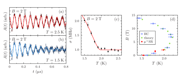
Figure 6: Sample TF µ${}^{\text{+}}$SR data measured for [Cu(HF${}_{\text{2}}$)(pyz)${}_{\text{2}}$]BF${}_{\text{4}}$ in an applied field of 2 T are shown in (a) and (b). Data are shown in the ‘rotating reference frame’, rotating at $\gamma_{\mathchoice{\hbox{\normalsize\textmu}}{\hbox{\normalsize\textmu}}{\hbox{\scriptsize\textmu}}{\hbox{\tiny\textmu}}}\times 1.9\mathrm{\;T}=\mathrm{257\;MHz}$, nearly cancelling out spin precession induced by the $2\mathrm{\;T}$ applied transverse field. (c) The evolution of the magnetic broadening $\sigma$ with $T$, showing a magnetic transition at 1.98 K in 2 T. (d) The $B$–$T$ phase diagram from Ref. Sengupta2009-nonmonotonic-TN-B-CuHF2pyz2BF4, showing the nonmonotonic behaviour at low applied magnetic field. In the key, HC is heat capacity, theory represents the results of computational modelling, and µ${}^{\text{+}}$SR  shows our results from TF measurements (see main text).

Although we expect the interplane exchange coupling $J_{\perp}$ to have a large amount of control of the thermodynamic properties of these materials, it may be the case that single-ion anisotropies are also responsible for deviations in the behaviour of our materials from the predictions of the 2DSLQHAF model. In particular, these anisotropies has been demonstrated to show a crossover to magnetic behaviour consistent with the 2D $XY$ model Xiao2009-XY-q2DHA . It was recently reported Sengupta2009-nonmonotonic-TN-B-CuHF2pyz2BF4 that [Cu(HF${}_{\text{2}}$)(pyz)${}_{\text{2}}$]BF${}_{\text{4}}$ exhibits an unusual nonmonotonic dependence of $T_{\mathrm{N}}$ as a function of applied magnetic field $B$ [see Fig. 6(d)]. This behavior was explained as resulting from the small $XY$-like anisotropy of the spin system in these systems. The physics of the unusual field-dependence then arises due to the dual effect of $B$ on the spins, both suppressing the amplitude of the order parameter by polarizing the spins along a given direction, and also reducing the phase fluctuations by changing the order parameter phase space from a sphere to a circle. A more detailed explanation for the behavior Sengupta2009-nonmonotonic-TN-B-CuHF2pyz2BF4 reveals that the energy scales of the physics are controlled by a Kosterlitz–Thouless-like mechanism, along with the interlayer exchange interaction $J_{\perp}$.

The measurement of the $B$–$T$ phase diagram in [Cu(HF${}_{\text{2}}$)(pyz)${}_{\text{2}}$]BF${}_{\text{4}}$ reported in Ref. Sengupta2009-nonmonotonic-TN-B-CuHF2pyz2BF4, was made by observing a small anomaly in specific heat. In order to test whether the phase boundary could be determined using muons, we carried out transverse-field (TF) µ${}^{\text{+}}$SR measurements using the LTF instrument at SµS. In these measurements, the field is applied perpendicular to the initial muon spin direction, causing a precession of the muon-spins in the sum of the applied and internal field directed perpendicular to the muon-spin orientation. Example TF spectra measured in a field of $2\mathrm{\;T}$ are shown in Fig. 6 (a) and (b). We find that the spectra are well described by a function

$$A(t)=A(0)\mathrm{e}^{-\sigma^{2}t^{2}/2}\cos(2\pi\nu t+\phi),$$ (8)

where the phase factor depends on the details of the detector geometry, and $\sigma$ is proportional to the second moment of the internal field distribution via $\sigma^{2}=\gamma_{\mathchoice{\hbox{\normalsize\textmu}}{\hbox{\normalsize\textmu}}{\hbox{\scriptsize\textmu}}{\hbox{\tiny\textmu}}}^{2}\langle B^{2}\rangle$. Upon cooling through $T_{\mathrm{N}}$ we see a large increase in $\sigma$, as shown in Fig. 6 (c). This approximately resembles an order parameter, and we identify the discontinuity at the onset of the increase with $T_{\mathrm{N}}$ by fitting $\sigma$ with the above-$T_{\mathrm{N}}$ relaxation adding in quadrature to the additional relaxation present below the transition. The resulting point at $T_{\mathrm{N}}(B=2\mathrm{\;T})=1.98(4)\mathrm{\;K}$ is shown to be consistent with the predicted low-field phase boundary in Fig. 6 (d). A further point, identifiable by its vertical rather than horizontal error bar, was found by performing a field scan at a fixed temperature of $T=1.8\mathrm{\;K}$. The field-dependence of the relaxation rate shows a sharp increase at the transition, at $B=1.5\pm 0.3\mathrm{\;T}$.

Points derived from µ${}^{\text{+}}$SR  measurements possibly lie slightly lower in $T$ than both that predicted by theory, and the line predicted on the basis of the specific heat measurements. The theoretical calculations use $J/k_{\mathrm{B}}=5.9\mathrm{\;K}$ and $J_{\perp}/J=2.5\times 10^{-3}$, whilst our estimates suggest $J/k_{\mathrm{B}}=6.3\mathrm{\;K}$ and $J_{\perp}/J=0.9\times 10^{-3}$. Performing these calculations for a purely 2D system results in the entire curve shifting to the left Sengupta2009-nonmonotonic-TN-B-CuHF2pyz2BF4 , and consequently the leftward shift of our data points is consistent with our finding of increased exchange anisotropy. It is clear that the TF µ${}^{\text{+}}$SR technique may be used in future to measure the $B$–$T$ phase diagram and enjoys some of the same advantages it has in ZF over specific heat and susceptibility in anisotropic systems.

III.4 Muon response for $T>T_{\mathrm{N}}$

M	X	$r_{\text{\textmu--F}}$ (nm)	$p_{1}$ (%)	$\sigma$ (MHz)	$T$ (K)
Cu	BF${}_{\text{4}}$	$0.1038(1)$	$77(1)$	$0.29(1)$	$5.1$
Cu	ClO${}_{\text{4}}$	$0.1081(2)$	$70(1)$	$0.37(1)$	$5.1$
Cu	PF${}_{\text{6}}$	$0.1044(2)$	$74(2)$	$0.29(2)$	$5.2$
Cu	AsF${}_{\text{6}}$	$0.1043(3)$	$78(2)$	$0.31(3)$	$4.9$
Cu	SbF${}_{\text{6}}$	$0.1047(2)$	$64(1)$	$0.30(1)$	$5.0$
Cu	BF${}_{\text{4}}$	$0.1042(1)$	$76(1)$	$0.26(1)$	$26$
Cu	ClO${}_{\text{4}}$	$0.1087(1)$	$71(1)$	$0.37(1)$	$25$
Cu	SbF${}_{\text{6}}$	$0.1080(3)$	$59(1)$	$0.26(1)$	$30$
Cu	NbF${}_{\text{6}}$	$0.1039(4)$	$69(3)$	$0.32(3)$	$32$
Cu	TaF${}_{\text{6}}$	$0.1039(2)$	$78(2)$	$0.26(3)$	$32$
Ni	SbF${}_{\text{6}}$	$0.1068(4)$	$60(1)$	$0.38(1)$	$19$
Ni	PF${}_{\text{6}}$	$0.1063(5)$	$66(2)$	$0.40(1)$	$8.4$

Table 2: Muon–fluorine dipole–dipole interaction fitted parameters in the family [M(HF${}_{\text{2}}$)(pyz)${}_{\text{2}}$]X, extracted from fitting data to Eq. (12). In addition to separation by metal ion, Cu compounds are grouped by the temperature at which the measurement was made: those compounds measured over a range of temperatures appear in both sections of the table.

Above $T_{\mathrm{N}}$, the character of the measured spectra changes considerably and we observe lower-frequency oscillations characteristic of the dipole–dipole interaction between muons and fluorine nuclei lancaster2007-muF . The Cu${}^{\text{2+}}$ electronic moments, which dominate the spectra for $T<T_{\mathrm{N}}$, are disordered in the paramagnetic regime and fluctuate very rapidly on the muon time scale. They are therefore motionally narrowed from the spectra, leaving the muon sensitive to the quasi-static nuclear magnetic moments.

A muon and nucleus interact via the two-spin Hamiltonian

$$\hat{H}=\sum_{i>j}\frac{\mu_{0}\gamma_{i}\gamma_{j}\hbar}{4\uppi r^{3}}\left[\bm{S}_{i}\cdot\bm{S}_{j}-3\left(\bm{S}_{i}\cdot\hat{\bm{r}}\right)\left(\bm{S}_{j}\cdot\hat{\bm{r}}\right)\right],$$ (9)

where the spins $\bm{S}_{i,j}$ with gyromagnetic ratios $\gamma_{i,j}$ are separated by the vector $\bm{r}$. This gives rise to a precession of the muon spin, and the muon-spin polarization along a quantization axis $z$ varies with time as

$$D_{z}(t)=\frac{1}{N}\left\langle\sum_{m,n}\left|\left\langle m\left|\sigma_{q}\right|n\right\rangle\right|^{2}\mathrm{e}^{\mathrm{i}\omega_{m,n}t}\right\rangle_{q},$$ (10)

where $N$ is the number of spin states, $\left|m\right\rangle$ and $\left|n\right\rangle$ are eigenstates of the total Hamiltonian $\hat{H}$, $\sigma_{q}$ is the Pauli spin matrix corresponding to the direction $q$, and $\left\langle\right\rangle_{q}$ represents an appropriately-weighted powder average. The vibrational frequency of the muon–fluorine bond exceeds by orders of magnitude both the frequencies observable in a µ${}^{\text{+}}$SR experiment, and the frequency appropriate to the dipolar coupling in Eq. (9); the bond length probed via these entangled states is thus time-averaged over thermal fluctuations. Fluorine is an especially strong candidate for this type of interaction firstly because it is highly electronegative causing the positive muon to stop close to fluorine ions, and secondly because its nuclei are 100% ${}^{\text{19}}$F, which has $I=\frac{1}{2}$.

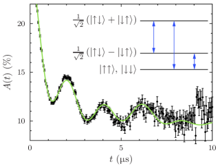
Figure 7: Data taken at $T=15\mathrm{\;K}\gg T_{\mathrm{N}}=1.4\mathrm{\;K}$ for [Cu(HF${}_{\text{2}}$)(pyz)${}_{\text{2}}$]BF${}_{\text{4}}$, showing Fµ oscillations along with a fit to Eq. (11). The inset shows the energy levels present in a simple system of two $S=\frac{1}{2}$ spins, along with the allowed transitions.

Data were fitted to a relaxation function

$$A(t)=A_{0}(p_{1}\mathrm{e}^{-\lambda_{\text{F--\textmu}}t}D_{z}(t)+p_{2}\mathrm{e}^{-\sigma^{2}t^{2}})+A_{\mathrm{bg}}\mathrm{e}^{-\lambda_{\mathrm{bg}}t},$$ (11)

where the amplitude fraction $p_{1}\approx 70\%$ reflects the muons stopping in a site or set of sites near to a fluorine nucleus, which result in the observed oscillations $D_{z}(t)$; the weak relaxation of the muon spins is crudely modelled by a decaying exponential. The fraction $p_{2}\approx 30\%$ describes those muons stopping in a class of sites primarily influenced by the randomly-orientated fields from other nuclear moments, giving rise to a Gaussian relaxation with $\sigma\approx 0.3\mathrm{\;MHz}$. Example data and a fit are shown in Fig. 7, whilst parameters extracted by fitting this function to data from each compound are shown in Table 2.

Fits to a variety of different $D_{z}(t)$ functions were attempted, including that resulting from a simple Fµ bond (previously observed in some polymers lancaster2009-FmuF-PTFE ) and the better-known FµF complex comprising a muon and two fluorine nuclei in linear symmetric configuration, which is seen in many alkali fluorides Brewer1986-FmuF . This latter model was also modified to include the possibilities of asymmetric and nonlinear bonds. Previous measurements lancaster2007-muF made in the paramagnetic regime of [Cu(HF${}_{\text{2}}$)(pyz)${}_{\text{2}}$]ClO${}_{\text{4}}$ suggested that the muon stopped close to a single fluorine in the HF${}_{\text{2}}$ group and also interacted with the more distant proton. This interaction is dominated by the F–µ  coupling and, for our fitting, the observed muon–fluorine dipole–dipole oscillations were found to be well described by a single Fµ interaction damped by a phenomenological relaxation factor. For such Fµ entanglement, the time evolution of the polarization is described by

$$D_{z}(t)=\frac{1}{6}\left[1+\sum_{j=1}^{3}u_{j}\cos\left(\omega_{j}t\right)\right],$$ (12)

where $u_{1}=2$, $u_{2}=1$ and $u_{3}=2$. The frequencies $\omega_{j}=j\omega_{\mathrm{d}}/2$, where $\omega_{\mathrm{d}}=\mu_{0}\gamma_{\mathchoice{\hbox{\normalsize\textmu}}{\hbox{\normalsize\textmu}}{\hbox{\scriptsize\textmu}}{\hbox{\tiny\textmu}}}\gamma_{\mathrm{F}}\hbar/4\uppi r^{3}$, in which $\gamma_{\mathrm{F}}=2\pi\times 2.518\times 10^{8}\mathrm{\;MHz\,T^{-1}}$ is the gyromagnetic ratio of a ${}^{\text{19}}$F nucleus NMR-Encyclopedia2002 , and $r$ is the muon–fluorine separation. These three frequencies arise from the three transitions between the three energy levels present in a system of two entangled $S=\frac{1}{2}$ particles (see inset to Fig. 7). The fact that the relaxation function is similar in all materials in the series, including [Cu(HF${}_{\text{2}}$)(pyz)${}_{\text{2}}$]ClO${}_{\text{4}}$ which is the only compound studied without fluorine in its anion, (the only difference being a slight lengthening of the µ–F bond, and with no significant change in oscillating fraction) suggests that the muon site giving rise to the Fµ oscillations in all systems is near the HF${}_{\text{2}}$ bridging ligand.

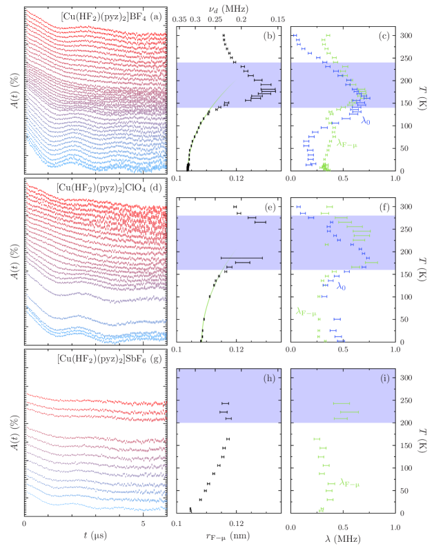
Figure 8: (a) Muon–fluorine dipole–dipole oscillations in [Cu(HF${}_{\text{2}}$)(pyz)${}_{\text{2}}$]BF${}_{\text{4}}$ over a temperature range $2\leq T\leq 300\mathrm{\;K}$. Asymmetry spectra are displaced vertically so as to approximately align with the temperature scale on plots (b) and (c). Ticks on the $y$-axis of (a) denote 1% asymmetry. Plot (b) shows the fitted value for $r_{\text{F--\textmu}}$ as a function of temperature. The line shown is a fit to the low-$T$ points with a $T^{2}$ scaling law, Eq. (14). The upper $x$-axis shows values of the dipole frequency, $\nu_{\mathrm{d}}$, which correspond to the lower $x$-axis values of $r_{\text{F--\textmu}}$. Plot (c) shows fitted relaxation rates $\lambda_{\text{F--\textmu}}$ and $\lambda_{0}$, referring to the relaxation of the Fµ function $D_{z}(t)$ in Eq. (11), and the pure relaxation in Eq. (13). Shaded regions indicate temperatures where $Q=2\uppi\lambda_{\text{F--\textmu}}/\omega_{\mathrm{d}}>2$, roughly parametrizing the disappearance of the oscillations. (d), (e) and (f) follow (a), (b) and (c), but show data for [Cu(HF${}_{\text{2}}$)(pyz)${}_{\text{2}}$]ClO${}_{\text{4}}$. (g), (h) and (i) similarly, but for [Cu(HF${}_{\text{2}}$)(pyz)${}_{\text{2}}$]SbF${}_{\text{6}}$ over the range $5\leq T\leq 250\mathrm{\;K}$. The $5\mathrm{\;K}$ $A(t)$ plot is omitted because the background is raised substantially by approach to the transition to LRO.

material	$r_{0}\mathrm{\;(nm)}$	$a\mathrm{\;(10^{-7}\,nm\,K^{-2}})$
[Cu(HF${}_{\text{2}}$)(pyz)${}_{\text{2}}$]BF${}_{\text{4}}$	$0.10376(3)$	$3.96(6)$
[Cu(HF${}_{\text{2}}$)(pyz)${}_{\text{2}}$]ClO${}_{\text{4}}$	$0.10842$	$2.7212$
PVDF lancaster2009-FmuF-PTFE	$0.10914$	$1.9488$

Table 3: Fitted values obtained by fitting muon–fluorine bond lengths with a $T^{2}$ scaling law, as Eq. (14).

The temperature evolution of the Fµ signal was studied for $T\leq 300\mathrm{\;K}$ in [Cu(HF${}_{\text{2}}$)(pyz)${}_{\text{2}}$]BF${}_{\text{4}}$ and [Cu(HF${}_{\text{2}}$)(pyz)${}_{\text{2}}$]ClO${}_{\text{4}}$. In both cases, the dipole–dipole oscillations disappear gradually in a temperature range $150\lesssim T\lesssim 250\mathrm{\;K}$, with oscillations totally absent in the center of this range, followed by reappearing as temperature is increased further. Plots of $A(t)$ spectra at a variety of temperatures are shown in Fig. 8 (a) and (d). The data were initially fitted to Eq. (11), with all parameters left free to vary. The temperature-evolution of the muon–fluorine bond length, $r_{\text{F--\textmu}}$, can be seen in Fig. 8 (b) and (e). The spectra were also fitted with

$$A(t)=A_{0}(p_{1}\mathrm{e}^{-\lambda_{0}t}+p_{2}\mathrm{e}^{-\sigma^{2}t^{2}})+A_{\mathrm{bg}}\mathrm{e}^{-\lambda_{\mathrm{bg}}t},$$ (13)

a sum of an exponential and a Gaussian relaxation, which might be expected to describe the data in the region where the oscillations vanish. Both this relaxation and that extracted from Eq. (11) are plotted in Fig. 8 (c) and (f), labelled $\lambda_{0}$ and $\lambda_{\text{F--\textmu}}$ respectively.

This bond length appears to grow and then shrink by nearly 20% over the $100\mathrm{\;K}$ range where the oscillations fade from the spectra and reappear. This variation is significantly larger than any variation in crystal lattice parameters which would be expected. Since the oscillations visibly disappear from the measured spectra, results from fitting with an oscillatory relaxation function are artifacts of the fitting procedure: since the frequencies scale with $1/r^{3}$, increasing bond length together with the associated relaxation rate fits the data with a suppressed oscillatory signal. This can be approximately quantified by examining the ratio $Q=2\uppi\lambda_{\text{F--\textmu}}/\omega_{\mathrm{d}}$, where a large value indicates that the function relaxes significantly before a single Fµ oscillation is completed. The shaded regions in Fig. 8 show where $Q>2$, which acts as an approximate bound on where the parametrization in Eq. (11) would be expected to fail. In the low-$T$ region where $Q<2$, the bond lengths appear to scale roughly as $T^{2}$, which has previously been observed in fluoropolymers lancaster2009-FmuF-PTFE . Parameters extracted from fitting to

$$r_{\text{F--\textmu}}=aT^{2}+r_{0}$$ (14)

are shown in Table 3.

The observation in these two samples of Fµ oscillations which disappear and then reappear is puzzling. While we have not identified a definitive mechanism, we can probably rule out an electronically mediated effect since, for $T\gg T_{\mathrm{N}}$, the Cu moment fluctuations will be outside the muon time-window. An explanation could involve nearby nuclear moments, possibly influenced by a thermally-driven structural distortion or instability.

A similar study of [Cu(HF${}_{\text{2}}$)(pyz)${}_{\text{2}}$]SbF${}_{\text{6}}$ is shown in Fig. 8 (g), (h) and (i). In this material, the oscillations appear not to vanish over the temperature range studied, though we cannot rule out a brief disappearance at $T\approx 200\mathrm{\;K}$. Instead, the oscillations show an apparently monotonic increase in damping with temperature, and the fitted bond length does not follow Eq. (14). The shaded region in Fig. 8 (h) and (i) has no upper bound, though we cannot rule out a constraint at $T>250\mathrm{\;K}$. The pure relaxation $\lambda_{0}$ is omitted because there is no region where the Fµ oscillations are sufficiently damped for Eq. (13) to be a good parametrization.

III.5 Muon site determination

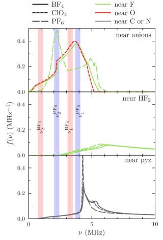
Figure 9: Probability density functions of muon precession frequencies at positions close to likely muon stopping sites in [Cu(HF${}_{\text{2}}$)(pyz)${}_{\text{2}}$]X with Cu${}^{\text{2+}}$ moments $\mu=\mu_{\mathrm{B}}$. The graphs show dipole fields near the fluorine or oxygen atoms in the negative anions; near the fluorine atoms in the bifluoride ligands; and near the carbon and nitrogen atoms, as a proxy for proximity to the pyrazine ring. The type of line indicates the compound for which the calculation was performed. The muon site is constrained to be close to particular atoms, indicated by line color. The shaded areas indicate ranges of fitted frequencies as $T\rightarrow 0$; two frequencies $\nu_{1,2}^{\mathrm{\mathrm{BF_{4}}}}$ represent those observed where X^- = BF${}_{\text{4}}^{-}$, and $\nu_{1,2}^{\mathrm{PF_{6}}}$ those observed in the X^- = PF${}_{\text{6}}^{-}$ analogue.

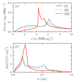
Figure 10: Probability density functions for muons in the putative oscillating sites near the pyrazine rings in [Cu(HF${}_{\text{2}}$)(pyz)${}_{\text{2}}$]BF${}_{\text{4}}$ (a) for muon precession frequency $\nu$ assuming that the moment on the copper site $\mu=\mu_{\mathrm{B}}$, created fom a histogram of dipole fields evaluated using Eq. (16) at points satisfying the constraints detailed in the text; and (b) for moment on the copper sites given the frequencies actually observed, evaluated using the pdfs in (a) and Eq. (18). Lines represent trial magnetic structures. All exhibit antiferromagnetic coupling through both the bifluoride and pyrazine exchange paths, whilst (i) has copper moments pointing at $45^{\circ}$ to the pyrazine grid, (ii) has moments along one of the pyrazine grid directions ($\bm{a}$ or $\bm{b}$), and (iii) has copper moments pointing along the bifluoride axis ($\bm{c}$).

Combining the data measured above and below the transition in these materials allows us to attempt to construct a self-consistent picture of possible muon sites. The observed dipole–dipole observations above $T_{\mathrm{N}}$ suggest that at least one muon stopping site is near a fluorine ion. We consider three classes of probable muon site: Class I sites near the fluorine ions in the HF${}_{\text{2}}$ groups, Class II sites near the pyrazine rings, and Class III sites near the anions at the centre of the pseudocubic pores. Comparison of Tables 1 and 2 show that the dominant amplitude component for $T>T_{\mathrm{N}}$ arises from dipole–dipole oscillatory component $p_{1}\mathrm{e}^{-\lambda t}D_{z}(t)$ and from the fast-relaxing component $p_{3}\mathrm{e}^{-\lambda_{3}t}$ for $T<T_{\mathrm{N}}$, and that these are comparable in amplitude. It is plausible therefore, to suggest that these two signals correspond to contributions from the same Class I muon sites near the HF${}_{\text{2}}$ groups. Moreover, the analysis of the $T>T_{\mathrm{N}}$ spectra in the previous section implies that this site lies $r_{\text{\textmu--F}}\approx 0.11\;\text{nm}$ from an F in the HF${}_{\text{2}}$ groups. The remainder of the signal (the oscillating fraction below $T_{\mathrm{N}}$ and the Gaussian relaxation above) can also be identified, suggesting that the sites uncoupled from fluorine nuclei (Classes II and/or III) result in the magnetic oscillations observed for $T<T_{\mathrm{N}}$.

We note further that the evidence from Fµ oscillations makes the occurence of Class III muon sites unlikely. The fact that spectra observed for $T>T_{\mathrm{N}}$ in the X^- = ClO${}_{\text{4}}^{-}$ material are nearly identical to those in all other compounds, in which X contains fluorine, suggest that the muons do not stop near the anions. Moreover, as discussed in Sec. IV and V below, we observe no Fµ oscillations in [Cu(pyz)${}_{\text{2}}$(pyo)${}_{\text{2}}$]X${}_{\text{2}}$ (Y^- = BF${}_{\text{4}}^{-}$, PF${}_{\text{6}}^{-}$) or [Cu(pyo)${}_{\text{6}}$](BF${}_{\text{4}}$)${}_{\text{2}}$, suggesting that muons do not stop preferentially near these fluorine-rich anions either. We therefore rule out the existence of Class III muon sites and propose that the magnetic oscillations measured for $T<T_{\mathrm{N}}$ most probably arise due to Class II sites found near the pyrazine ligands.

Below $T_{\mathrm{N}}$, the measured muon precession frequencies allow us to determine the magnetic field at these Class II muon sites via $\nu=\gamma_{\mathchoice{\hbox{\normalsize\textmu}}{\hbox{\normalsize\textmu}}{\hbox{\scriptsize\textmu}}{\hbox{\tiny\textmu}}}B/2\pi$. Simulating the magnetic field inside the crystal therefore allows us to compare these $B$-fields with those predicted for likely magnetic structures and may permit us to constrain the ordered moment. For the case of our ZF measurements in the antiferromagnetic state, the local magnetic field at the muon site $\bm{B}_{\mathrm{local}}$ is given by

$$\bm{B}_{\mathrm{local}}=\bm{B}_{\mathrm{dipole}}+\bm{B}_{\mathrm{hyperfine}},$$ (15)

where $\bm{B}_{\mathrm{dipole}}$ is the dipolar field from magnetic ions located within a large sphere centred on the muon site and $\bm{B}_{\mathrm{hyperfine}}$ the contact hyperfine field caused by any spin density overlapping with the muon wavefunction. This spin density is difficult to estimate accurately, particularly in complex molecular systems, but it is probable for insulating materials such as these that the spin density on the copper ion is well localised and so we ignore the hyperfine contribution in our analysis. The dipole field $\bm{B}_{\mathrm{dipole}}$ is a function of the coordinate of the muon site $\bm{r}_{\mathchoice{\hbox{\normalsize\textmu}}{\hbox{\normalsize\textmu}}{\hbox{\scriptsize\textmu}}{\hbox{\tiny\textmu}}}$, and comprises a vector sum of the fields from each of the magnetic ions in the crystal approximated as a point dipole, so that

$$\bm{B}_{\mathrm{dipole}}(\bm{r}_{\mathchoice{\hbox{\normalsize\textmu}}{\hbox{\normalsize\textmu}}{\hbox{\scriptsize\textmu}}{\hbox{\tiny\textmu}}})=\mu\sum_{i}\frac{\mu_{0}}{4\uppi r^{3}}\left[3(\hat{\bm{\mu}}_{i}\cdot\hat{\bm{r}})\hat{\bm{r}}-\hat{\bm{\mu}}_{i}\right],$$ (16)

where $\bm{r}=\bm{r}_{i}-\bm{r}_{\mathchoice{\hbox{\normalsize\textmu}}{\hbox{\normalsize\textmu}}{\hbox{\scriptsize\textmu}}{\hbox{\tiny\textmu}}}$ is the relative position of the muon and the $i^{\text{th}}$ ion with magnetic moment $\bm{\mu}_{i}=\mu\hat{\bm{\mu}}_{i}$, and $i$ is an index implying summation over all of the ions which make up the crystal.

Although these materials are known to be antiferromagnetic from their negative Curie–Weiss temperatures and zero spontaneous magnetization at low temperatures Manson2009-Cu-SbF6 ; manson2006-CuHF2pyz2BF4-chemcomm , their magnetic structures are unknown. Dipole field simulations were therefore performed for a variety of trial magnetic structures with $\mu=\mu_{\mathrm{B}}$. We analyse the results of these calculations using a probabilistic method. We begin by allowing the possibility that the magnetic precession signal could arise from any of the possible classes of muon site identified above. Random positions in the unit cell were generated and dipole fields calculated at these. To prevent candidate sites lying too close to atoms we constrain all sites such that $r_{\mathchoice{\hbox{\normalsize\textmu}}{\hbox{\normalsize\textmu}}{\hbox{\scriptsize\textmu}}{\hbox{\tiny\textmu}}\text{--\emph{A}}}>0.1\mathrm{\;nm}$ where $A$ is any atom. Possible Class I muon sites were identified with $r_{\text{\textmu--F}}=r_{0}\pm 0.01\mathrm{\;nm}$ (where $r_{0}$ is the muon–fluorine distance established from Fµ oscillations) and possible Class II sites were selected with the constraint that $0.10\leq r_{\text{\textmu--C,N}}\leq 0.12\mathrm{\;nm}$. The predicted probability density function (pdf) of muon precession frequencies (resulting from the magnitudes of the calculated fields) are plotted in Fig. 9, with the observed frequencies superimposed. Results are shown for a trial magnetic structure comprising copper spins lying in the plane of the pyrazine layers and at $45^{\circ}$ to the directions of the pyrazine chains, and with spins arranged antiferromagnetically both along those chains and along the HF${}_{\text{2}}$ groups. This candidate structure is motivated by analogy with [Cu(pyz)${}_{\text{2}}$](ClO${}_{\text{4}}$)${}_{\text{2}}$, which also comprises Cu${}^{\text{2+}}$ ions in layers of 2D pyrazine lattices Tsyrulin2010-Cu(pz)2(ClO4)2 , and with the parent phases of the cuprate superconductors Kastner1998-cuprates-review , which are also two-dimensional Heisenberg systems of $S=\frac{1}{2}$ Cu${}^{\text{2+}}$ ions. Other magnetic structures investigated give qualitatively similar results. From Fig. 9 it is clear that the only sites with significant probability density near to the observed frequencies are those lying near the anions (i.e. Class III sites) which we have argued are not compatible with our data. The more plausible muon sites correspond to higher frequencies than those observed. Our conclusion is that it is likely that the Cu${}^{\text{2+}}$ moments are rather smaller than the $\mu_{\mathrm{B}}$ assumed in the initial calculation.

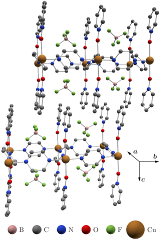
Figure 11: Structure of [Cu(pyz)${}_{\text{2}}$(pyo)${}_{\text{2}}$](BF${}_{\text{4}}$)${}_{\text{2}}$. Copper ions lie in 2D square layers, bound by pyrazine rings. Pyridine-N-oxide ligands protrude from the coppers in a direction approximately perpendicular to these layers. Tetrafluoroboride ions fill the pores remaining in the structure. Ion sizes are schematic; copper ions are shown twice as large for emphasis, and hydrogens have been omitted for clarity.

If we accept that the muon sites giving rise to magnetic precession are near the pyrazine groups then we may use this calculation to constrain the size of the copper moment. Since $\nu$ is obtained from experiment, what we would like to know is $g(\mu|\nu)$, the pdf of copper moment $\mu$ given the observed $\nu$. This can be obtained from our calculated $f(\nu/\mu)$ using Bayes’ theorem Sivia2006-Bayes , which yields

$$g(\mu|\nu)=\frac{\frac{1}{\mu}f(\nu/\mu)}{\int_{0}^{\mu_{{\rm max}}}\frac{1}{\mu^{\prime}}f(\nu/\mu^{\prime})\,{\rm d}\mu^{\prime}}\,,$$ (17)

where we have assumed a prior probability for the copper moment that is uniform between zero and $\mu_{{\rm max}}$. We take $\mu_{{\rm max}}=2\mu_{{\rm B}}$, although our results are insensitive to the precise value of $\mu_{{\rm max}}$ as long as it is reasonably large. When multiple frequencies $\{\nu_{i}\}$ are present in the spectra, it is necessary to multiply their probabilities of observation in order to obtain the chance of their simultaneous observation, so we evaluate

$$g(\mu|\{\nu_{i}\})\propto\prod_{i}\int_{\nu_{i}-\Delta\nu_{i}}^{\nu_{i}+\Delta\nu_{i}}f(\nu_{i}/\mu)\,{\rm d}\nu_{i}\,,$$ (18)

where $\Delta\nu_{i}$ is the error on the fitted frequency. Results are shown in Fig. 10, along with the dipole field pdfs which gave rise to them. By inspection of the pdfs, the copper moment is likely to be $\mu\lesssim 0.5\mu_{\mathrm{B}}$. The dipole field simulations results also lend weight to our contention that the oscillatory signal cannot arise from the sites that also lead to the Fµ component above-$T_{\mathrm{N}}$. If this were the case then the most likely moment on the copper would be $\mu_{\mathrm{Cu}}\lesssim 0.2\mu_{\mathrm{B}}$, which seems unreasonably small. We note that moment sizes of $\mu\lesssim 0.5\mu_{\mathrm{B}}$ were also observed for the 2DSLQHA system La${}_{\text{2}}$CuO${}_{\text{4}}$ (a recent estimate Reehuis2006-neutron-high-B-La2CuO4 from neutron diffraction gave $[0.42\pm 0.01]\mu_{\mathrm{B}}$), despite the predictions of $0.6\mu_{\mathrm{B}}$ from spin wave theory and Quantum Monte Carlo Chakravarty1989-2DHA-moment-size . It was suggested in that case Chakravarty1989-2DHA-moment-size that disorder might play a role in reducing the moment sizes; an additional possible mechanism for this suppression is ring exchange Motrunich2005-ring-exchange-triangular-lattice ; Katanin2002-ring-exchange-La2CuO4 .

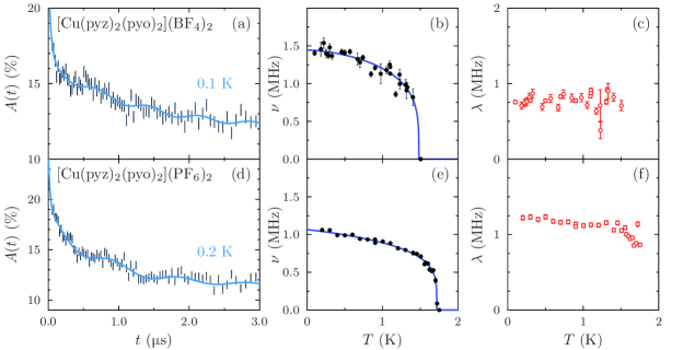
Figure 12: Example data and fits for [Cu(pyz)${}_{\text{2}}$(pyo)${}_{\text{2}}$]Y${}_{\text{2}}$. From left to right: (a) and (d) show sample asymmetry spectra $A(t)$ for $T<T_{\mathrm{N}}$ along with a fit to Eq. (19); (b) and (e) show the frequency $\nu$ as a function of temperature; and (c) and (f) show relaxation rates $\lambda_{i}$ as a function of temperature. The relaxation rates $\lambda_{1}$, associated with the oscillation, and $\lambda_{3}$, the fast-relaxing initial component, do not vary significantly with $T$ and are not shown. Only a slight trend in $\lambda_{2}$ in the Y^- = PF${}_{\text{6}}^{-}$ material [graph (f)] is observed.

One limitation of this analysis is that the mechanism for magnetic coupling of copper ions through the pyrazine rings is postulated to be via spin exchange, in which small magnetic polarisations are induced on intervening atoms Lloret1998-spin-pol-pyz-pyd . Density functional theory calculations estimate that these are small, with the nitrogen and carbon moments estimated at $\mu_{\mathrm{C}}\approx 0.01\mu_{\mathrm{B}}$ and $\mu_{\mathrm{N}}\approx 0.07\mu_{\mathrm{B}}$, respectively Middlemiss2008-CuHF2pyz2BF4-DFT . However, their effect may be non-negligible: they may be significantly closer to the muon site than a copper moment, and dipole fields fall off rapidly, as $1/r^{3}$. Further, since much of the electron density in a pyrazine ring is delocalised in $\uppi$-orbitals, the moments may not be point-like, as assumed in our dipole field calculations. Further, this may lead to overlap of spin density at the muon site and result in a nonzero hyperfine field.

IV $\text{[Cu(pyz)}_{\text{2}}\text{(pyo)}_{\text{2}}\text{]\emph{Y}}_{\text{2}}$

In this section, we report the magnetic behavior of another family of molecular systems which shows quasi-2D magnetism, but for which the interlayer groups are very different and arranged in a completely different structure, resulting in a 2D coordination polymer. This system is [Cu(pyz)${}_{\text{2}}$(pyo)${}_{\text{2}}$]Y${}_{\text{2}}$, where Y^- = BF${}_{\text{4}}^{-}$, PF${}_{\text{6}}^{-}$. As with the previous case, $S=\frac{1}{2}$ Cu${}^{\text{2+}}$ ions are bound in a 2D square lattice of [Cu(pyz)${}_{\text{2}}$]${}^{\text{2+}}$ sheets lying in the $ab$-plane. Pyridine-N-oxide (pyo) ligands [shown in Fig. 1 (b)] protrude from the copper ions along the $c$-direction, perpendicular to the $ab$-plane in the Y^- = PF${}_{\text{6}}^{-}$ material, but making an angle $\beta-90\approx 29^{\circ}$ with the normal in Y^- = BF${}_{\text{4}}^{-}$. The anions then fill the pores remaining in the structure. The structure of [Cu(pyz)${}_{\text{2}}$(pyo)${}_{\text{2}}$](BF${}_{\text{4}}$)${}_{\text{2}}$ is shown in Fig. 11.

In a typical synthesis, an aqueous solution of CuY${}_{\text{2}}$ hydrate (Y^- = BF${}_{\text{4}}^{-}$ or PF${}_{\text{6}}^{-}$) was combined with an ethanol solution that contained a mixture of pyrazine and pyridine-N-oxide or 4-phenylpyridine-N-oxide. Deep blue-green solutions were obtained in each case, and when allowed to slowly evaporate at room temperature for a few weeks, dark green plates were recovered in high yield. Crystal quality could be improved by sequential dilution and collection of multiple batches of crystals from the original mother liquor. The relative amounts of pyz and pyo were optimized in order to prevent formation of compounds such as CuY${}_{\text{2}}$(pyz)${}_{\text{2}}$ or [Cu(pyo)${}_{\text{6}}$]Y${}_{\text{2}}$.

Samples were measured in the LTF apparatus at SµS. Example data measured on [Cu(pyz)${}_{\text{2}}$(pyo)${}_{\text{2}}$]Y${}_{\text{2}}$ are shown in Fig. 12, where we observe oscillations in $A(t)$ at a single frequency below $T_{\mathrm{N}}$. Data were fitted to a relaxation function

$$A(t)=A_{0}\left(p_{1}\cos(2\uppi\nu_{1}t)\mathrm{e}^{-\lambda_{1}t}+p_{2}\mathrm{e}^{-\lambda_{2}t}+p_{3}\mathrm{e}^{-\lambda_{3}t}\right)+A_{\mathrm{bg}}.$$ (19)

The small amplitude fraction $p_{1}<10\%$ for both samples refers to muons stopping in a site or set of sites with a narrow distribution of quasi-static local magnetic fields, giving rise to the oscillations; $p_{2}\approx 50\%$ is the fraction of muons stopping in a class of sites giving rise to a large relaxation rate $30\lesssim\lambda\lesssim 60$ MHz and $p_{3}\approx 50\%$ represents the fraction of muons stopping in sites with a small relaxation rate $\lambda_{3}\approx 1\;\mathrm{MHz}$. The data from these compounds fit best with $\phi=0$, and it is thus omitted from this expression. Frequencies obtained from fitting the data to Eq. (19) were then modelled with Eq. (4). The results of these fits are shown Fig. 12, and Table 4.

Our results show that [Cu(pyz)${}_{\text{2}}$(pyo)${}_{\text{2}}$](BF${}_{\text{4}}$)${}_{\text{2}}$ has a transition temperature $T_{\mathrm{N}}=1.5\pm 0.1\mathrm{\;K}$ and a quasi-static magnetic field at the muon site $\nu_{1}(T=0)=1.4\pm 0.1\mathrm{\;MHz}$. No quantities other than $\nu_{1}$ show a significant trend in the temperature region $0.1\leq T\leq 1.6\mathrm{\>K}$. Above the transition, purely relaxing spectra are observed, displaying no Fµ oscillations. As suggested above, this makes the existence of muon sites near the anions unlikely. We find a critical exponent of $\beta=0.25\pm 0.10$, where the large uncertainty results in part from the difficulty in fitting the $A(t)$ data in the critical region.

Our results for [Cu(pyz)${}_{\text{2}}$(pyo)${}_{\text{2}}$](PF${}_{\text{6}}$)${}_{\text{2}}$ show that the transition temperature is slightly higher at $T_{\mathrm{N}}=1.72\pm 0.02\mathrm{\;K}$ and the oscillations occur at a lower frequency of $\nu_{1}(T=0)=1.07\pm 0.03\mathrm{\;MHz}$. The relaxation rates $\lambda_{2}$ and $\lambda_{3}$ also decrease in magnitude as temperature is increased, settling on roughly constant values $\lambda_{2}\approx 0.6\mathrm{\;MHz}$ and $\lambda_{3}\approx 15\mathrm{\;MHz}$ for $T>T_{\mathrm{N}}$. No other quantities show a significant trend in the temperature region $0.2\leq T\leq 1.7\mathrm{\>K}$. Above the transition, relaxing spectra devoid of Fµ oscillations are again observed. The critical exponent $\beta=0.22\pm 0.02$.

The small amplitude of the oscillations, common to both samples, might be explained in a number of ways. The materials may undergo long-range ordering but there may be an increased likelihood of stopping in sites where the magnetic field nearly precisely cancels. Alternatively, a range of similar muon sites may be present with a large distribution of frequencies, or alternatively the presence of dynamics, washing out any clear oscillations in large fractions of the spectra and instead resulting in a relaxation. Finally, we cannot exclude the possibility that only a small volume of the sample undergoes a magnetic transition; this may indicate the presence of a small impurity phase, possibly located at either grain boundaries or, given that this is a powder sample, near the crystallites’ surfaces. We note also that the behavior of fitted parameters in these materials is qualitatively similar to that reported in CuCl${}_{\text{2}}$(pyz), where there is also a relatively small precessing fraction of muons and little variation in relaxation rates as $T_{\mathrm{N}}$ is approached from below Lancaster2004-CuX2(pyz)-and-0DMMs .

V $\text{[Cu(pyo)}_{\text{6}}\text{]\emph{Z}}_{\text{2}}$

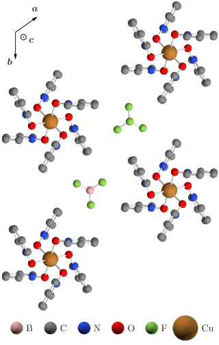
Figure 13: Structure of [Cu(pyo)${}_{\text{6}}$](BF${}_{\text{4}}$)${}_{\text{2}}$, viewed along the three-fold ($\bm{c}$-) axis, after Ref. Reinen1979-Cupyo6X2, . Copper ions are surrounded by octahedra of six oxygens, each part of a pyridine-N-oxide ligand; [Cu(pyo)${}_{\text{6}}$]${}^{\text{2+}}$ complexes space-pack with BF${}_{\text{4}}^{-}$ stabilising the structure. Ion sizes are schematic; copper ions are shown twice as large for emphasis, and hydrogens have been omitted for clarity. As indicated in the top left, the $\bm{a}$ and $\bm{b}$ directions lie in the plane of the paper, separated by $\gamma=120^{\circ}$, whilst the $\bm{c}$ direction is out of the page.

The next example is not a coordination polymer, but instead forms a three-dimensional structure of packed molecular groups. The molecular magnet [Cu(pyo)${}_{\text{6}}$]Z${}_{\text{2}}$, where Z^- = BF${}_{\text{4}}^{-}$, ClO${}_{\text{3}}^{-}$, PF${}_{\text{6}}^{-}$, comprises Cu${}^{\text{2+}}$ ions on a slightly distorted cubic lattice, located in [Cu(pyo)${}_{\text{6}}$]${}^{\text{2+}}$ complexes, and surrounded by octahedra of oxygen atoms Algra1978-Cupyo6X2 . The structure is shown in 13. This approximately cubic structure, which arises from the molecules’ packing, might suggest that a three-dimensional model of magnetism would be appropriate. In fact, although the observed bulk properties of [M(pyo)${}_{\text{6}}$]X${}_{\text{2}}$ where M${}^{\text{2+}}$  = Co${}^{\text{2+}}$, Ni${}^{\text{2+}}$ or Fe${}^{\text{2+}}$ are largely isotropic, but the copper analogues display quasi–low-dimensional, $S=\frac{1}{2}$ Heisenberg antiferromagnetism Algra1978-Cupyo6X2 . Weakening of superexchange in certain directions, and thus the lowering of the systems’ effective dimensionality, is attributed to lengthening of the superexchange pathways resulting from Jahn–Teller distortion of the Cu–O octahedra, which is observed in structural and EPR measurements Wood1980-Cupyo6X2 ; Reinen1979-Cupyo6X2 . At high temperatures, ($T\gtrsim\mathrm{100\;K})$, these distortions are expected to be dynamic but, as $T$ is reduced (to $\approx 50\mathrm{\;K}$), they freeze out. The anion Z^- determines the nature of the static Jahn–Teller elongation. The Z^- = BF${}_{\text{4}}^{-}$ material displays ferrodistortive ordering which, in combination with the antiferromagnetic exchange, gives rise to 2D Heisenberg antiferromagnetic behavior Algra1978-Cupyo6X2 ; Burriel1990-Cupyo6BF4-susceptibility . By contrast, Z^- = ClO${}_{\text{4}}^{-}$, NO${}_{\text{3}}^{-}$ (neither of which is investigated here) display antiferrodistortive ordering Wood1980-Cupyo6X2 , which gives rise to quasi-1D Heisenberg antiferromagnetism Algra1978-Cupyo6X2 . All of the samples investigated were measured in the LTF spectrometer at SµS.

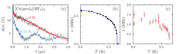
Figure 14: Example data and fits for [Cu(pyo)${}_{\text{6}}$](BF${}_{\text{4}}$)${}_{\text{2}}$. From left to right: (a) shows sample asymmetry spectra $A(t)$ for $T<T_{\mathrm{N}}$ and $T>T_{\mathrm{N}}$, along with fits to Eq. (19) and Eq. (20), respectively; (b) shows frequency as a function of temperature; and (c) shows relaxation rate $\lambda_{2}$ as a function of temperature; $\lambda_{1}$ was held fixed during the fitting procedure, and $\lambda_{3}$ persists for $T>T_{\mathrm{N}}$. In the $\nu(T)$ plot, error bars are included on the points but in most cases they are smaller than the marker being used.

In the Z^- = BF${}_{\text{4}}^{-}$ compound, below a temperature $T_{\mathrm{N}}$, a single oscillating frequency is observed, indicating a transition to a state of long-range magnetic order. Example data above and below the transition, along with fits, are shown in Fig. 14 (a). Data were fitted to Eq. (19), and the frequencies extracted from the procedure fitted as a function of temperature to Eq. (4)as shown in Fig. 14 (b). This procedure identifies a transition temperature $T_{\mathrm{N}}=0.649\pm 0.005\mathrm{\;K}$. The only other parameter found to vary significantly in the range $20\mathrm{\;mK}\leq T\leq T_{\mathrm{N}}$ was $\lambda_{2}$, shown in as shown in Fig. 14 (c). The fitted parameters are shown in Table 4. We may compare this with the result of an earlier low-temperature specific heat study Algra1978-Cupyo6X2 which found a very small $\lambda$-point anomaly at $T_{\mathrm{N}}=0.62\pm 0.01\mathrm{\;K}$, slightly lower than our result. Fitting the magnetic component of the heat capacity with the predictions from a two-dimensional Heisenberg antiferromagnet gives $J/k_{\mathrm{B}}=-1.10\pm 0.02\mathrm{\;K}$, and similar analysis of the magnetic susceptibility Algra1978-Cupyo6X2 yields $J/k_{\mathrm{B}}=-1.08\pm 0.03\mathrm{\;K}$. Using these values, together with the muon estimate of $T_{\mathrm{N}}$ and Eq. (6), allows us to estimate the inter-plane coupling, $J_{\perp}/J=0.26\pm 0.01$. (Using the value of $T_{\mathrm{N}}$ from heat capacity results in an estimate $J_{\perp}/J=0.21\pm 0.02$.)

For temperatures $T_{\mathrm{N}}<T\leq 1\mathrm{\;K}$, the spectra are well described by a relaxation function

$$A(t)=A_{0}(p_{1}\mathrm{e}^{-\lambda t}+p_{2}\mathrm{e}^{-\sigma^{2}t^{2}})+A_{\mathrm{bg}},$$ (20)

comprising an initial fast-relaxing component with $\lambda\approx 20\mathrm{\mathrm{\;MHz}}$, and a Gaussian relaxation with $\sigma\approx 0.4\mathrm{\;MHz}$ corresponding to the slow depolarisation of muon spins due to randomly-orientated nuclear moments.

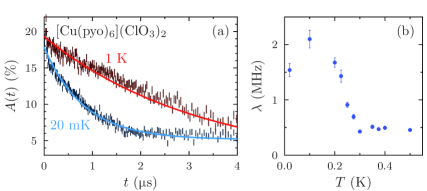
Figure 15: Example data and fits for [Cu(pyo)${}_{\text{6}}$](ClO${}_{\text{3}}$)${}_{\text{2}}$. Representative $A(t)$ spectra for $T<T_{\mathrm{N}}$ and $T>T_{\mathrm{N}}$, along with fits to Eq. (21), are shown in (a), whilst the value of the relaxation rate, $\lambda$, as a function of temperature is shown in (b).

The Z^- = ClO${}_{\text{3}}^{-}$ material also shows evidence for a magnetic transition, although in this case we do not observe oscillations in the muon asymmetry. Instead we measure a discontinuous change in the relaxation which seems to point towards an ordering transition. Example asymmetry spectra are shown in Fig. 15 (a) and data at all measured temperatures are well described with the relaxation function

$$A(t)=A_{0}\mathrm{e}^{-\lambda t}+A_{\mathrm{bg}}\,.$$ (21)

Evidence for a magnetic transition comes from the temperature evolution of $\lambda$ [Fig. 15(b)], where we see that the relaxation decreases with increasing temperature until it settles at $T\approx 0.3\mathrm{\;K}$, on a value $\lambda\approx 0.5\mathrm{\;MHz}$. It is likely that this tracks the internal magnetic field inside the material, and is suggestive of $T_{\mathrm{N}}=0.30\pm 0.01\mathrm{\;K}$.

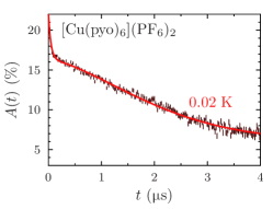
Figure 16: Sample asymmetry spectrum for [Cu(pyo)${}_{\text{6}}$](PF${}_{\text{6}}$)${}_{\text{2}}$ measured at $T=0.02\mathrm{\;K}$. The spectra remain indistinguishable from this across the range of temperatures examined, $0.02\mathrm{\;K}\leq T\leq 1\mathrm{\;K}$.

The final member of this family studied, Z^- = PF${}_{\text{6}}^{-}$, shows no evidence for a magnetic transition over the range of temperatures studied, $0.02\mathrm{\;K}\leq T\leq 1\mathrm{\;K}$. An example spectrum is shown in Fig. 16. The data resemble the above-transition data measured in the BF${}_{\text{4}}$ and ClO${}_{\text{3}}$ compounds and it therefore seems likely that the paramagnetic state persists to the lowest temperature measured.

VI $\text{Ag(pyz)}_{\text{2}}\text{(S}_{\text{2}}\text{O}_{\text{8}}\text{)}$

The examples so far have used Cu${}^{\text{2+}}$ (3d${}^{\text{9}}$) as the magnetic species. An alternative strategy is to employ Ag${}^{\text{2+}}$ (4d${}^{\text{9}}$) which also carries an $S=\frac{1}{2}$ moment. This idea has led to the synthesis of Ag(pyz)${}_{\text{2}}$(S${}_{\text{2}}$O${}_{\text{8}}$), which comprises square sheets of [Ag(pyz)${}_{\text{2}}$]${}^{\text{2+}}$ units spaced with S${}_{\text{2}}$O${}_{\text{8}}$${}^{\text{2}-}$ anions Manson2009-Agpyz2S2O8 . Each silver ion lies at the centre of an elongated (AgN${}_{\text{4}}$O${}_{\text{2}}$) octahedron, where the Ag–N bonds are significantly shorter than the Ag–O. Preparation details can be found in Ref. Matthews1971-Ag-Cu-Co-Ni-pyz-prep, .

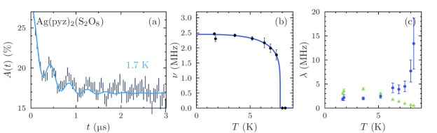
Figure 17: Example data and fits for Ag(pyz)${}_{\text{2}}$(S${}_{\text{2}}$O${}_{\text{8}}$). From left to right: (a) shows sample asymmetry spectra $A(t)$ for $T<T_{\mathrm{N}}$ along with a fit to Eq. (22); (b) shows the frequency as a function of temperature; and (c) shows relaxation rates $\lambda_{i}$ as a function of temperature. Filled circles show the relaxation rate $\lambda_{1}$, which relaxes the oscillation. The filled triangles correspond to the relaxation $\lambda_{2}$.

Measurements were made using the GPS instrument at SµS. Example muon data, along with fits to various parameters, are shown in Fig. 17. Asymmetry oscillations are visible in spectra taken below a transition temperature $T_{\mathrm{N}}$. The data were fitted with a relaxation function

$$A(t)=A_{0}\left(p_{1}\cos(2\uppi\nu_{1}t+\phi_{1})\mathrm{e}^{-\lambda_{1}t}+p_{2}\mathrm{e}^{-\lambda_{2}t}\right)+A_{\mathrm{bg}},$$ (22)

comprising a single damped oscillatory component, a slow-relaxing component, and a static background signal. The onset of increased relaxation $\lambda_{1}$ as the transition is approached from below leads to large statistical errors on fitted values, as is evident in Fig. 17 (c). The relaxation $\lambda_{2}$ decreases with increasing temperature. Fitting to Eq. (4) allows the critical parameters $\beta=0.19\pm 0.02$ and $T_{\mathrm{N}}=7.8\pm 0.3\mathrm{\;K}$ to be determined. Fitted values are shown in Table 4.

The in-plane exchange $J$ is too large to be determined with pulsed fields Manson2009-Agpyz2S2O8 : $M(B)$ does not saturate in fields up to $64\mathrm{\;T}$. However, fitting $\chi(T)$ data allows an estimate of the exchange $J/k_{\mathrm{B}}\approx 53\mathrm{\;K}$ (and thus, in conjunction with $g$ measured by EPR, the saturation field $B_{\mathrm{c}}$ is estimated to be $160\mathrm{\;T}$). Thus, $k_{\mathrm{B}}T_{\mathrm{N}}/J=0.148\pm 0.006$. Estimation of the exhange anisotropy with Eq. (6) yields $|J_{\perp}/J|\sim 10^{-6}$, but this very small ratio of ordering temperature to exchange strength is outside the range in which the equation is known to yield accurate results. The alternative method of parametrizing the low dimensionality in terms of correlation length at the Néel temperature (see Sec. III.2) yields $\xi(T_{\mathrm{N}})/a=1000\pm 300$.

VII $\text{[Ni(HF}_{\text{2}}\text{)(pyz)}_{\text{2}}\text{]\emph{X}}$

material	$\nu_{1}\mathrm{\,(MHz)}$	$p_{1}$	$p_{2}$	$p_{3}$	$T_{\mathrm{N}}\mathrm{\,(K)}$	$\beta$	$\alpha$	$J/k_{\mathrm{B}}\mathrm{\>(K)}$	$|J_{\perp}/J|$
[Cu(pyz)${}_{\text{2}}$(pyo)${}_{\text{2}}$](BF${}_{\text{4}}$)${}_{\text{2}}$	$1.4(1)$	$<10$	$50$	$50$	$1.5(1)$	$0.25(10)$	$1.6(3)$	-	-
[Cu(pyz)${}_{\text{2}}$(pyo)${}_{\text{2}}$](PF${}_{\text{6}}$)${}_{\text{2}}$	$0.64(1)$	$<10$	$50$	$50$	$1.72(2)$	$0.22(2)$	$1.1(3)$	$8.1(3)$ *	$2\times 10^{-4}$
[Cu(pyo)${}_{\text{6}}$](BF${}_{\text{4}}$)${}_{\text{2}}$	$0.599(5)$	$15$	$30$	$55$	$0.649(5)$	$0.29(1)$	$1.7(1)$	$1.09(2)$ †	$0.23(2)$
Ag(pyz)${}_{\text{2}}$(S${}_{\text{2}}$O${}_{\text{8}}$)	$2.45(4)$	$30$	$70$	-	$7.8(3)$	$0.19(2)$	$3(2)$	$52.7(3)$	$\sim 10^{-6}$

Table 4: Fitted parameters for molecular magnets in the family [Cu(pyz)${}_{\text{2}}$(pyo)${}_{\text{2}}$]Y${}_{\text{2}}$, [Cu(pyo)₆](BF₄)₂ and Ag(pyz)${}_{\text{2}}$(S${}_{\text{2}}$O${}_{\text{8}}$). The first parameters shown relate to fits to Eq. (19) (for the first three rows) or Eq. (22) [for Ag(pyz)${}_{\text{2}}$(S${}_{\text{2}}$O${}_{\text{8}}$)]. This allows us to derive frequencies at $T=0$, $\nu_{i}$; and probabilities of stopping in the various classes of stopping site, $p_{i}$, in percent. Then, the temperature dependence of $\nu_{i}$ is fitted with Eq. (4), extracting values for the Néel temperature, $T_{\mathrm{N}}$, critical exponent $\beta$ and parameter $\alpha$. Finally, the quoted $J/k_{\mathrm{B}}$ is obtained from pulsed-field experiments goddard2008-2DHMexchange The asterisk (*) indicates the value of $J$ was obtained using $g_{ab}=2.04(1)$ in conjunction with single-crystal pulsed-field data. The dagger (^†) indicates that the value of $J$ is extracted from heat capacity and susceptibility from Ref. Algra1978-Cupyo6X2, .). The ratio of inter- to in-plane coupling, $J_{\perp}/J$, is obtained by combining $T_{\mathrm{N}}$ and $J$ with formulae extracted from quantum Monte Carlo simulations (see Sec. III.2, and Ref. goddard2008-2DHMexchange, ). The dash in the $p_{3}$ column for Ag(pyz)${}_{\text{2}}$(S${}_{\text{2}}$O${}_{\text{8}}$) reflects the fact that there is no third component in Eq. (22). Dashes in the $J/k_{\mathrm{B}}$ and $J_{\perp}/J$ columns for [Cu(pyz)${}_{\text{2}}$(pyo)${}_{\text{2}}$](BF${}_{\text{4}}$)${}_{\text{2}}$ indicate a lack of pulsed-field data for this material.

In order to investigate the influence of a different spin state on the magnetic cation in the [M(HF${}_{\text{2}}$)(pyz)${}_{\text{2}}$]X architecture the [Ni(HF${}_{\text{2}}$)(pyz)${}_{\text{2}}$]X (X^- = PF${}_{\text{6}}^{-}$, SbF${}_{\text{6}}^{-}$) system has been synthesised Manson2011-NiHF2pyz2X . These materials are isostructural with the copper family discussed in Sec. III, but contain $S=1$ Ni${}^{\text{2+}}$ cations.

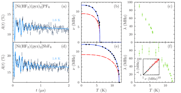
Figure 18: Example data and fits for M = Ni magnets. From left to right: (a) and (d) show sample asymmetry spectra $A(t)$ for $T<T_{\mathrm{N}}$ along with a fit to Eq. (3); (b) and (e) show frequencies as a function of temperature [no data points are shown for the second line because this frequency $\nu_{2}$ was held in fixed proportion to the first, $\nu_{1}$ (see text)]; and (c) and (f) show relaxation rate $\lambda_{3}$ as a function of temperature. In the $\nu(T)$ plot, error bars are included on the points but in most cases they are smaller than the marker being used. The inset to (f) shows $\nu_{2}\equiv\nu$ plotted against $\lambda_{3}\equiv\lambda$ on a log–log scale. The black line shows $\lambda=\nu^{2}$ .

X	$T_{\mathrm{N}}\mathrm{\>(K)}$	$\nu_{1}\mathrm{\>(MHz)}$	$\nu_{2}\mathrm{\>(MHz)}$	$\lambda_{3}\mathrm{\;(MHz)}$	$p_{1}$	$p_{2}$	$p_{3}$	$\beta$	$\alpha$
PF${}_{\text{6}}$	$6.0(4)$	$12.0$	$9.3$	$90$	$15$	$10$	$75$	$0.25(10)$	$2.8(2)$
SbF${}_{\text{6}}$	$12.26(1)$	$12.3(1)$	$8.98(1)$	$80$	$25$	$10$	$65$	$0.34(4)$	$3.1(1)$

Table 5: Fitted parameters for M = Ni magnets. Errors shown are statistical uncertainties on fitting and thus represent lower bounds. Errors on Ni…PF${}_{\text{6}}$ could not be estimated due to the fitting procedure (see text).

Data were taken using the GPS spectrometer at PSI. Example data are shown in Fig. 18. We observe oscillations at two frequencies below the materials’ respective ordering temperatures. Data were fitted with a relaxation function

$$A(t) = A_{0}\left[p_{1}\mathrm{e}^{-\lambda_{1}t}\cos(2\pi\nu_{1}t)+p_{2}\mathrm{e}^{-\lambda_{2}t}\cos(2\pi P_{2}\nu_{1}t)\right.$$ (23)

$$\left.+p_{3}\mathrm{e}^{-\lambda_{3}t}\right]+A_{\mathrm{bg}}\mathrm{e}^{-\lambda_{\mathrm{bg}}t}.$$

Of those muons which stop in the sample, $p_{1}\approx 25\%$ indicates the fraction of the signal corresponding to the low-frequency oscillating state with $\nu_{1}(T=0)\approx 12.3\mathrm{\>MHz}$; $p_{2}\approx 10\%$ corresponds to muons stopping in the high-frequency oscillating state with $\nu_{2}(T=0)\approx 9.0\mathrm{\;MHz}$; and $p_{3}\approx 65\%$ represents muons stopping in a site with a large relaxation rate $\lambda_{3}(T=0)\approx 70\mathrm{\;MHz}$. The frequencies were observed to scale with one-another, and consequently the second frequency was held in fixed proportion $\nu_{2}=P_{2}\nu_{1}$ during the fitting procedure. The only other parameter which changes significantly in value below $T_{\mathrm{N}}$ is $\lambda_{3}$, which decreases with a trend qualitatively similar to that of the frequencies. Fitting the extracted frequencies to Eq. (4) allows the transition temperature $T_{\mathrm{N}}=12.25\pm 0.03\mathrm{\>K}$ and critical exponent $\beta=0.34\pm 0.04$ to be extracted. In contrast to the copper family studied in Sec. III, the relation $\lambda\propto\nu^{2}$ holds true, suggesting that a field distribution whose width diminishes with increasing temperature is responsible for the variation in $\lambda$, and that dynamics are relatively unimportant in determining the muon response. This is shown graphically in the inset to Fig. 18 (f), where a plot of frequency against relaxation rate lies on top of a line representing a $\lambda=\nu^{2}$ relationship. The phase $\phi$ required in previous fits (e.g. Eq. (3)) is not necessesary in fitting these spectra, and is set to zero. Fitted parameters are shown in Table 5.

Data for the X^- = PF${}_{\text{6}}^{-}$ compound was subject to similar analysis, fitting spectra below $T_{\mathrm{N}}$ to Eq. (23), this time with $p_{1}\approx 15\%$, $\nu_{1}(T=0)\approx 12.0\mathrm{\>MHz}$; $p_{2}\approx 10\%$, $\nu_{2}(T=0)\approx 9.3\mathrm{\>MHz}$; and $p_{3}\approx 75\%$, $\lambda_{3}(T=0)\approx 100\mathrm{\;MHz}$. The phase $\phi$ again proved unnecessary. These spectra do not show as sharp a transition as the X^- = SbF${}_{\text{6}}^{-}$ compound, with the oscillating fraction of the signal decaying rather before the appearance of spectra whose different character indicates clearly that the sample is above $T_{\mathrm{N}}$. The available data do not allow reliable extraction of critical parameters, but we estimate $5.5\mathrm{\;K}\leq T_{\mathrm{N}}\leq 6.2\mathrm{\;K}$ and $0.15\leq\beta\leq 0.4$. Fitted values are shown in Table 5.

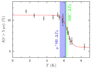
Figure 19: The asymmetry at late times $A(t>5\mathrm{\;\mathchoice{\hbox{\normalsize\textmu}}{\hbox{\normalsize\textmu}}{\hbox{\scriptsize\textmu}}{\hbox{\tiny\textmu}}s)}$ measured in Ni(HF${}_{\text{2}}$)(pyz)${}_{\text{2}}$PF${}_{\text{6}}$ along with a fit to Eq. (24). Overlaid are regions corresponding to the range of values found by fitting the frequency of oscillations as a function of temperature with Eq. (4) ($5.5\mathrm{\;K}\leq T_{\mathrm{N}}\leq 6.2\mathrm{\;K}$), and the value of the $\lambda$-like anomaly in specific heat capacity (SHC) measurements with a representative error of $0.1\mathrm{\;K}$ ($6.1\mathrm{\;K}\leq T_{\mathrm{N}}\leq 6.3\mathrm{\;K}$). The darker area represents the overlap between these regions.

Another method to locate the transition is to observe a transition in the amplitude of the muon spectra at late times to observe the transition as a function of temperature from zero in the unordered state to the ‘$\frac{1}{3}$-tail’ characteristic of LRO, described in Sec. II. Spectra were fitted with the simple relaxation function $A(t>5\mathrm{\;\mathchoice{\hbox{\normalsize\textmu}}{\hbox{\normalsize\textmu}}{\hbox{\scriptsize\textmu}}{\hbox{\tiny\textmu}}s})=A_{\mathrm{bg}}\mathrm{e}^{-\lambda_{\mathrm{bg}}t}$, and then the amplitudes obtained fitted with a Fermi-like step function

$$A(t>5\mathrm{\;\mathchoice{\hbox{\normalsize\textmu}}{\hbox{\normalsize\textmu}}{\hbox{\scriptsize\textmu}}{\hbox{\tiny\textmu}}s},\;T)=A_{2}+\frac{A_{1}-A_{2}}{\mathrm{e}^{(T-T_{\mathrm{mid}})/w}+1}\,,$$ (24)

which provides a method of modelling a smooth transition between $A_{1}=A(T<T_{\mathrm{N}})$ and $A_{2}=A(T>T_{\mathrm{N}})$. The fitted amplitudes and Fermi function are shown in Fig. 19 (c). The fitted mid-point $T_{\mathrm{mid}}=6.4\pm 0.1\mathrm{\;K}$, and width $w=0.3\pm 0.1\mathrm{\;K}$. Spin relaxation peaks just above $T_{\mathrm{N}}$, and so one would expect that $T_{\mathrm{N}}$ lies at the lower end of this transition. Thus, the µ${}^{\text{+}}$SR analysis suggests $T_{\mathrm{N}}=6.1\pm 0.3\mathrm{\;K}$ (i.e. $T_{\mathrm{mid}}-w\pm w$). This is consistent with the estimate from $\nu_{i}(T)$ and the value $T_{\mathrm{N}}=6.2\mathrm{\;K}$ obtained from heat capacity Manson2011-NiHF2pyz2X .

Members of the M = Ni family exhibit Fµ oscillations rather like their copper counterparts, with a similar fraction of the muons in sites giving rise to dipole–dipole interactions. The results of these fits are shown along with those from Cu compounds in Table 2. Because the nickel data were measured at temperatures different from those of the copper compounds and, as described in Sec. III.4, the muon–fluorine bond length in the compound is sensitive to changes in temperature, care must be taken when comparing these values to those of the Cu family. Linearly interpolating the bond lengths for [Cu(HF${}_{\text{2}}$)(pyz)${}_{\text{2}}$]SbF${}_{\text{6}}$ at $9\mathrm{\;K}$ and $29\mathrm{\;K}$ to find an approximate value of the bond length at $19\mathrm{\;K}$ yields $r_{\text{\textmu--F}}(T=19\mathrm{\;K})=0.1062\pm 0.0002\mathrm{\;nm}$ (where the error represents a combination of the statistical errors on the fits and variation recorded in thermometry, and is thus a lower bound), very similar to that measured for [Ni(HF${}_{\text{2}}$)(pyz)${}_{\text{2}}$]SbF${}_{\text{6}}$, $r_{\text{\textmu--F}}(T=19\mathrm{\;K})=0.1068\pm 0.0004\mathrm{\;nm}$.

In spite of being isostructural to the [Cu(HF${}_{\text{2}}$)(pyz)${}_{\text{2}}$]X systems, the dimensionality of these Ni variants is ambiguous. Susceptibility data fit acceptably to a number of models, and ab initio theoretical calculations are suggestive of one-dimensional behavior, dominated by the exchange along the bifluoride bridges. This is discussed more fully in Ref. Manson2011-NiHF2pyz2X, .

VIII Discussion

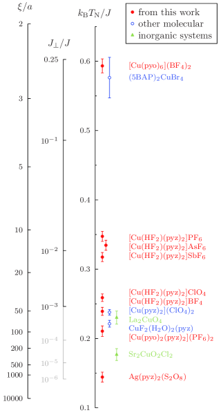
Figure 20: Quantification of the two-dimensionality of the materials in this paper and comparison with other notable 2DSLQHA systems. Filled circles show materials investigated in this paper; open circles show other molecular materials; and filled triangles show inorganic systems. The low dimensionality is parametrized firstly with the directly experimental ratio $T_{\mathrm{N}}/J$, and then with predictions quantum Monte Carlo simulations for both the exchange anisotropy, $J_{\perp}/J$ [Eq. (6)], and the correlation length of an ideal 2D Heisenberg antiferromagnet with the measured $J$ at a temperature $T_{\mathrm{N}}$ [Eq. (7)]. The greying-out of the axis for $J_{\perp}/J$ indicates where Eq. (6) is extrapolated beyond the range for which it was originally derived yasuda2005-2DHA-JvsTN . Values of $T_{\mathrm{N}}/J$ for the other materials were evaluated from Refs. Woodward2001-5BAP2CuBr4, ; Greven1995-Sr2CuO2Cl2, ; Aeppli1989-La2CuO4-Ba-doping, .

Fig. 20 collects the results from this paper and shows how isolation between two-dimensional layers varies over a variety of systems; those presented in this paper, molecular materials studied elsewhere, and inorganic materials. The primary axis is the experimental ratio $T_{\mathrm{N}}/J$. Also shown are the ratios of the in-plane and inter-plane exchange interactions, $J_{\perp}/J$, and the correlation length at the transition, $\xi(T_{\mathrm{N}})/a$, extracted from fits to quantum Monte Carlo simulations. Of the materials in this paper, the least anisotropic is [Cu(pyo)${}_{\text{6}}$](BF${}_{\text{4}}$)${}_{\text{2}}$, whose low transition temperature is caused by a small exchange constant rather than particularly high exchange anisotropy. The members of the [Cu(HF${}_{\text{2}}$)(pyz)${}_{\text{2}}$]X family with octahedral anions have $k_{\mathrm{B}}T_{\mathrm{N}}/J\approx 0.33$, rather more than the $k_{\mathrm{B}}T_{\mathrm{N}}/J\approx 0.25$ shown by their counterparts with tetrahedral anions (as has been noted previously goddard2008-2DHMexchange ). This makes the latter comparable to highly 2D molecular systems [Cu(pyz)${}_{\text{2}}$](ClO${}_{\text{4}}$)${}_{\text{2}}$ and CuF${}_{\text{2}}$(H${}_{\text{2}}$O)${}_{\text{2}}$(pyz), and the cuprate parent compound La${}_{\text{2}}$CuO${}_{\text{4}}$. Below this, [Cu(pyo)${}_{\text{2}}$(pyz)${}_{\text{2}}$](PF${}_{\text{6}}$)${}_{\text{2}}$ exhibits a ratio $k_{\mathrm{B}}T_{\mathrm{N}}/J\approx 0.21(1)$. The prototypical inorganic 2D system Sr${}_{\text{2}}$CuO${}_{\text{2}}$Cl${}_{\text{2}}$ exhibits $k_{\mathrm{B}}T_{\mathrm{N}}/J=0.177\pm 0.009$, and thus $\xi(T_{\mathrm{N}})/a=280\pm 90$. The most 2D material investigated in this paper, Ag(pyz)${}_{\text{2}}$(S${}_{\text{2}}$O${}_{\text{8}}$), has $k_{\mathrm{B}}T_{\mathrm{N}}/J=0.148\pm 0.006$, implying $\xi(T_{\mathrm{N}})/a=1000\pm 300$, with the added benefit that the magnetic field required to probe its interactions is far closer to the range of fields achievable in the laboratory. By these measures, molecular magnets provide some excellent realizations of the 2DSLQHA, with Ag(pyz)${}_{\text{2}}$(S${}_{\text{2}}$O${}_{\text{8}}$) being the best realization found to date.

Another method of examining the dimensionality of these systems is to consider their behavior in the critical region. The critical exponent $\beta$ is a quantity frequently extracted in studies of magnetic materials, and it is often used to make inferences about the dimensionality of the system under study. In the critical region near a magnetic transition, an order parameter $\Phi$, identical to the (staggered) magnetization, would be expected to vary as

$$\Phi(T)=\Phi_{0}\left(1-\frac{T}{T_{\mathrm{N}}}\right)^{\beta}.$$ (25)

In simple, isotropic cases, the value of $\beta$ depends on the dimensionality of the system, $d$, and that of the order parameter, $D$. For example, in the 3D Heisenberg model ($d=3$, $D=3$), $\beta=0.367$, whilst in the 2D Ising model ($d=2$, $D=1$), $\beta=\frac{1}{8}$. Since the muon precession frequency is proportional to the local field, it is also proportional to the moment on the magnetic ions in a crystal, and can be used as an effective order parameter. However, Eq. (25) would only be expected to hold true in the critical region. The extent of the critical region (defined as that region where simple mean-field theory does not apply) can be parametrized by the Ginzburg temperature $T_{\mathrm{G}}$, which is related to the transition temperature $T_{\mathrm{c}}$ by Chaikin-and-Lubensky

$$\frac{|T_{\mathrm{G}}-T_{\mathrm{c}}|}{T_{\mathrm{c}}}=\left[\left(\frac{\xi}{a}\right)^{d}\left(\frac{\Delta C}{k_{\mathrm{B}}}\right)\right]^{\frac{2}{d-4}},$$ (26)

where $d$ is the dimensionality, $\xi$ is the correlation length and $\Delta C$ is the discontinuity in the heat capacity. Quantum Monte Carlo simulations suggest sengupta2003-bulkmeasuresbad that $\Delta C/k_{\mathrm{B}}\approx J_{\perp}/J$. It follows that for $d=3$, where $\Delta C/k_{\mathrm{B}}\approx 1$ we have $\left|T_{\mathrm{G}}-T_{\mathrm{c}}\right|/T_{\mathrm{c}}\approx(\xi/a)^{-6}$, giving rise to a narrow critical region. In two dimensions, we have $\left|T_{\mathrm{G}}-T_{\mathrm{c}}\right|/T_{\mathrm{c}}\approx(\xi/a)^{-2}(\Delta C/k_{\mathrm{B}})^{-1}$. Anisotropic materials with small $J_{\perp}/J$ only show a small heat capacity discontinuity, while $\xi/a$ grows according to Eq. (7). This leads to a $\left|T_{\mathrm{G}}-T_{\mathrm{c}}\right|/T_{\mathrm{c}}$ of order 1 for our materials, that is, a larger critical region for 2D (as compared to 3D) systems.

The large critical region in these materials allows meaningful critical parameters to be extracted from muon data. The simplest method of doing so is to fit the data to Eq. (4), as we have throughout this study; alternatively, critical scaling plots can be used (e.g. Ref. Pratt2007-critical-behaviour-CoGly, ), which we have performed, finding the results are unchanged within error. Since $\beta$ might be expected to give an indication of the dimensionality of the hydrodynamical fluctuations in these materials, a comparison between extracted $\beta$ and exchange anisotropy parametrized by $k_{\mathrm{B}}T_{\mathrm{N}}/J$ is shown in Fig. 21. Members of the [Cu(HF${}_{\text{2}}$)(pyz)${}_{\text{2}}$]X family show some correlation between the critical exponent and the effective dimensionality but overall, the relationship is weak. This is probably because $\beta$, which is not a Hamiltonian parameter, is not simply a function of the dimensionality of the interactions, but probes the nature of the critical dynamics (including propagating and diffusive modes) which could differ substantially between systems.

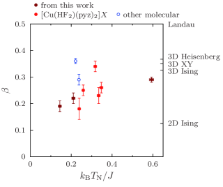
Figure 21: Critical exponent $\beta$, as commonly extracted from Eq. (4), plotted against the experimental ratio $k_{\mathrm{B}}T_{\mathrm{N}}/J$, indicative of exchange anisotropy. Bright filled circles indicate [Cu(HF${}_{\text{2}}$)(pyz)${}_{\text{2}}$]X materials examined in Sec. III, whilst darker circles indicate other materials studied in this work: [Cu(pyz)${}_{\text{2}}$(pyo)${}_{\text{2}}$]BF${}_{\text{4}}$ (Sec. IV); [Cu(pyo)${}_{\text{6}}$](BF${}_{\text{4}}$)${}_{\text{2}}$ (Sec. V); Ag(pyz)${}_{\text{2}}$(S${}_{\text{2}}$O${}_{\text{8}}$) (Sec. VI). Open circles indicate other molecular materials: CuF${}_{\text{2}}$(H${}_{\text{2}}$O)${}_{\text{2}}$(pyz) (Ref. Manson2008-CuF2(H2O)2(pyz), ); [Cu(pyz)${}_{\text{2}}$](ClO${}_{\text{4}}$)${}_{\text{2}}$ (Ref. lancaster2007-CuPz2ClO42, ).

IX Conclusions

We have presented a systematic study of muon-spin relaxation measurements on several families of quasi two-dimensional molecular antiferromagnet, comprising ligands of pyrazine, bifluoride and pyridine-N-oxide; and the magnetic metal cations Cu${}^{\text{2+}}$, Ag${}^{\text{2+}}$ and Ni${}^{\text{2+}}$. In each case µ${}^{\text{+}}$SR  has been shown to be sensitive to the transition temperature $T_{\mathrm{N}}$, which is often difficult to unambiguously identify with specific heat and magnetic susceptibility measurements. We have combined these measurements with predictions of quantum Monte Carlo calculations to identify the extent to which each is a good realization of the 2DSLQHA model. The critical parameters derived from following the temperature evolution of the µ${}^{\text{+}}$SR  precession frequencies do not show a strong correlation with the degree of isolation of the 2D magnetic layers.

The analysis of magnetic ordering in zero applied field in terms of inter-layer coupling $J_{\perp}$ presented here does not take into account the effect of single-ion–type anisotropy on the magnetic order. This has been suggested to be important close to $T_{\mathrm{N}}$ in several examples of 2D molecular magnet Xiao2009-XY-q2DHA where it causes a crossover to $XY$-like behavior. In fact, its influence is confirmed in the nonmonotonic $B$–$T$ phase diagram seen in [Cu(HF${}_{\text{2}}$)(pyz)${}_{\text{2}}$]BF${}_{\text{4}}$. It is likely that this is one factor that determines the ordering temperature of a system, although, as shown in Ref. Xiao2009-XY-q2DHA, , it is a smaller effect than the interlayer coupling parametrized by $J_{\perp}$. The future synthesis of single crystal samples of these materials will allow the measurement of the single-ion anisotropies for the materials studied here.

The presence of muon–fluorine dipole–dipole oscillations allows the determination of some muon sites in these materials, although it appears from our results that these are not those that lead to magnetic oscillations. However, the Fµ  signal has been shown to be useful in identifying transitions at temperatures well above the magnetic ordering transition, which appear to have a structural origin. The fluorine oscillations hamper the study of dynamic fluctuations above $T_{\mathrm{N}}$, which often appear as a residual relaxation on top of the dominant nuclear relaxation. It may be possible in future to use RF radiation to decouple the influence of the fluorine from the muon ensemble to allow muons to probe the dynamics.

The muon-spin precession signal, upon which much of the analysis presented here is based, is seen most strongly in the materials containing Cu${}^{\text{2+}}$ and is more heavily relaxed in the Ni${}^{\text{2+}}$ materials. This is likely due to the larger spin value in the Ni-containing materials. This is borne out by measurements on pyz-based materials containing Mn and Fe ions Lancaster2006-Mndca2pyz-and-FeNCS2pyz2 , where no oscillations are observed, despite the presence of magnetic order shown unambiguously by other techniques. In the case of Mn-containing materials magnetic order is found with µ${}^{\text{+}}$SR  through a change in relative amplitudes of relaxing signals due to a differerence in the nature of the relaxation on either side of the transition. It is likely, therefore that muon studies of molecular magnetic materials containing ions with small spin quantum numbers will be most fruitful in the future.

Finally, the temperature dependence of the relaxation rates in these materials has been shown to be quite complex, reflecting the variety of muon sites in these systems. In favourable cases these data could be used to probe critical behavior, such as critical slowing down, although the unambiguous identification of such behavior may be problematic.

Despite these limitations on the use of µ${}^{\text{+}}$SR  in examining molecular magnetic systems of the type studied here, it is worth stressing that the technique still appears uniquely powerful in providing insights into the magnetic behavior of these materials and will certainly be useful in the future as a wealth of new systems are synthesised and the goal of microscopically engineering such materials is approached.

- (1) E. Manousakis, Rev. Mod. Phys. 63, 1 (Jan 1991)
- (2) Note that, in this model, the exchange energy in a bond between two parallel spins is . The sums are therefore over unconstrained values of and . They include an implicit factor of to prevent double-counting, leading to the form in Eq. (1).
- (3) N. D. Mermin and H. Wagner, Phys. Rev. Lett. 17, 1133 (Nov 1966), http://link.aps.org/doi/10.1103/PhysRevLett.17.1133
- (4) V. L. Berezinskii, Sov. Phys. JETP 32, 493 (1971)
- (5) P. Sengupta, A. W. Sandvik, and R. R. P. Singh, Phys. Rev. B 68, 094423 (Sep 2003), http://prola.aps.org/abstract/PRB/v68/i9/e094423
- (6) S. J. Blundell, T. Lancaster, F. L. Pratt, P. J. Baker, M. L. Brooks, C. Baines, J. L. Manson, and C. P. Landee, J. Phys. Chem. Solids 68, 2039 (2007), ISSN 0022-3697, http://www.sciencedirect.com/science/article/B6TXR-4PJ6GRS-4/2/5323eeff%81018ca9f644d9eacbf4234a
- (7) P. A. Goddard, J. Singleton, P. Sengupta, R. D. McDonald, T. Lancaster, S. J. Blundell, F. L. Pratt, S. Cox, N. Harrison, J. L. Manson, H. I. Southerland, and J. A. Schlueter, New Journal of Physics 10, 083025 (2008), http://stacks.iop.org/1367-2630/10/083025
- (8) T. Lancaster, S. J. Blundell, M. L. Brooks, P. J. Baker, F. L. Pratt, J. L. Manson, M. M. Conner, F. Xiao, C. P. Landee, F. A. Chaves, S. Soriano, M. A. Novak, T. P. Papageorgiou, A. D. Bianchi, T. Herrmannsdorfer, J. Wosnitza, and J. A. Schlueter, Phys. Rev. B 75, 094421 (2007), http://link.aps.org/abstract/PRB/v75/e094421
- (9) T. Lancaster, S. J. Blundell, M. L. Brooks, P. J. Baker, F. L. Pratt, J. L. Manson, C. P. Landee, and C. Baines, Phys. Rev. B 73, 020410 (2006), http://link.aps.org/abstract/PRB/v73/e020410
- (10) S. J. Blundell and F. L. Pratt, J. Phys. Condens. Mat. 16, R771 (2004), http://stacks.iop.org/0953-8984/16/i=24/a=R03
- (11) F. Xiao, F. M. Woodward, C. P. Landee, M. M. Turnbull, C. Mielke, N. Harrison, T. Lancaster, S. J. Blundell, P. J. Baker, P. Babkevich, and F. L. Pratt, Phys. Rev. B 79, 134412 (Apr 2009)
- (12) P. Sengupta, C. D. Batista, R. D. McDonald, S. Cox, J. Singleton, L. Huang, T. P. Papageorgiou, O. Ignatchik, T. Herrmannsdörfer, J. L. Manson, J. A. Schlueter, K. A. Funk, and J. Wosnitza, Phys. Rev. B 79, 060409 (Feb 2009)
- (13) S. J. Blundell, Contemp. Phys. 40, 175 (May 1999), http://www.informaworld.com/smpp/content~content=a713806540
- (14) J. L. Manson, M. M. Conner, J. A. Schlueter, T. Lancaster, S. J. Blundell, M. L. Brooks, F. L. Pratt, T. Papageorgiou, A. D. Bianchi, J. Wosnitza, and M.-H. Whangbo, Chem. Commun., 4894(2006), http://dx.doi.org/10.1039/b608791d
- (15) J. L. Manson, J. A. Schlueter, K. A. Funk, H. I. Southerland, B. Twamley, T. Lancaster, S. J. Blundell, P. J. Baker, F. L. Pratt, J. Singleton, R. D. McDonald, P. A. Goddard, P. Sengupta, C. D. Batista, L. Ding, C. Lee, M.-H. Whangbo, I. Franke, S. Cox, C. Baines, and D. Trial, J. Am. Chem. Soc. 131, 6733 (2009), http://pubs.acs.org/doi/abs/10.1021/ja808761d
- (16) J. L. Manson, S. H. Lapidus, P. W. Stephens, P. K. Peterson, K. E. Carreiro, H. I. Southerland, T. Lancaster, S. J. Blundell, A. J. Steele, P. A. Goddard, F. L. Pratt, J. Singleton, Y. Kohama, R. D. McDonald, R. E. D. Sesto, N. A. Smith, J. Bendix, S. A. Zvyagin, J. Kang, C. Lee, M.-H. Whangbo, V. S. Zapf, and A. Plonczak, Inorg. Chem. 50, 5990 (2011), http://pubs.acs.org/doi/abs/10.1021/ic102532h
- (17) R. S. Hayano, Y. J. Uemura, J. Imazato, N. Nishida, T. Yamazaki, and R. Kubo, Phys. Rev. B 20, 850 (Aug 1979), http://prola.aps.org/abstract/PRB/v20/i3/p850_1
- (18) F. L. Pratt, P. J. Baker, S. J. Blundell, T. Lancaster, M. A. Green, and M. Kurmoo, Phys. Rev. Lett. 99, 017202 (Jul 2007)
- (19) T. Lancaster, S. J. Blundell, D. Andreica, M. Janoschek, B. Roessli, S. N. Gvasaliya, K. Conder, E. Pomjakushina, M. L. Brooks, P. J. Baker, D. Prabhakaran, W. Hayes, and F. L. Pratt, Phys. Rev. Lett. 98, 197203 (2007), http://link.aps.org/abstract/PRL/v98/e197203
- (20) T. Lancaster, S. J. Blundell, F. L. Pratt, C. H. Gardiner, W. Hayes, and A. T. Boothroyd, J. Phys. Condens. Mat. 15, 8407 (2003), http://stacks.iop.org/0953-8984/15/8407
- (21) T. Lancaster, S. J. Blundell, F. L. Pratt, M. L. Brooks, J. L. Manson, E. K. Brechin, C. Cadiou, D. Low, E. J. L. McInnes, and R. E. P. Winpenny, J. Phys. Condens. Mat. 16, S4563 (2004), http://stacks.iop.org/0953-8984/16/i=40/a=009
- (22) T. Lancaster, S. J. Blundell, M. L. Brooks, P. J. Baker, F. L. Pratt, J. L. Manson, and C. Baines, Phys. Rev. B 73, 172403 (May 2006)
- (23) J. Major, J. Mundy, M. Schmolz, A. Seeger, K. Döring, K. Fürderer, M. Gladisch, D. Herlach, and G. Majer, Hyperfine Interact. 31, 259 (1986), ISSN 0304-3843, http://dx.doi.org/10.1007/BF02401569
- (24) A. Amato, Rev. Mod. Phys. 69, 1119 (Oct 1997)
- (25) J. Sugiyama, M. Månsson, Y. Ikedo, T. Goko, K. Mukai, D. Andreica, A. Amato, K. Ariyoshi, and T. Ohzuku, Phys. Rev. B 79, 184411 (May 2009), http://link.aps.org/doi/10.1103/PhysRevB.79.184411
- (26) S. J. Blundell, Magnetism in condensed matter (Oxford University Press, 2001)
- (27) C. Yasuda, S. Todo, K. Hukushima, F. Alet, M. Keller, M. Troyer, and H. Takayama, Phys. Rev. Lett. 94, 217201 (Jun 2005)
- (28) P. Hasenfratz and F. Niedermayer, Phys. Lett. B 268, 231 (1991), ISSN 0370-2693, http://www.sciencedirect.com/science/article/B6TVN-472JMYX-TK/2/e93851a%c0aad5cab1217b0751e0e4b76
- (29) B. B. Beard, R. J. Birgeneau, M. Greven, and U.-J. Wiese, Phys. Rev. Lett. 80, 1742 (Feb 1998)
- (30) M. A. Kastner, R. J. Birgeneau, G. Shirane, and Y. Endoh, Rev. Mod. Phys. 70, 897 (Jul 1998)
- (31) T. Lancaster, S. J. Blundell, P. J. Baker, M. L. Brooks, W. Hayes, F. L. Pratt, J. L. Manson, M. M. Conner, and J. A. Schlueter, Phys. Rev. Lett. 99, 267601 (2007), http://link.aps.org/abstract/PRL/v99/e267601
- (32) T. Lancaster, F. L. Pratt, S. J. Blundell, I. McKenzie, and H. E. Assender, J. Phys. Condens. Mat. 21, 346004 (2009), http://stacks.iop.org/0953-8984/21/i=34/a=346004
- (33) J. H. Brewer, S. R. Kreitzman, D. R. Noakes, E. J. Ansaldo, D. R. Harshman, and R. Keitel, Phys. Rev. B 33, 7813 (Jun 1986), http://link.aps.org/doi/10.1103/PhysRevB.33.7813
- (34) D. M. Grant and R. K. Harris, Encyclopedia of Nuclear Magnetic Resonance, Volume 9, Advances in NMR (Wiley, 2002) ISBN 9780471490821
- (35) J. L. Manson, J. A. Schlueter, K. A. Funk, H. I. Southerland, B. Twamley, T. Lancaster, S. J. Blundell, P. J. Baker, F. L. Pratt, J. Singleton, R. D. McDonald, P. A. Goddard, P. Sengupta, C. D. Batista, L. Ding, C. Lee, M.-H. Whangbo, I. Franke, S. Cox, C. Baines, and D. Trial, J. Am. Chem. Soc. 131, 6733 (2009), http://pubs.acs.org/doi/abs/10.1021/ja808761d
- (36) N. Tsyrulin, F. Xiao, A. Schneidewind, P. Link, H. M. Ronnow, J. Gavilano, C. P. Landee, M. M. Turnbull, and M. Kenzelmann, Phys. Rev. B 81, 134409 (Apr 2010)
- (37) D. Sivia and J. Skilling, Data Analysis: A Bayesian Tutorial, 2nd ed. (OUP, 2006) ISBN 978-0-19-856832-2
- (38) M. Reehuis, C. Ulrich, K. Prokeš, A. Gozar, G. Blumberg, S. Komiya, Y. Ando, P. Pattison, and B. Keimer, Phys. Rev. B 73, 144513 (Apr 2006), http://link.aps.org/doi/10.1103/PhysRevB.73.144513
- (39) S. Chakravarty, B. I. Halperin, and D. R. Nelson, Phys. Rev. B 39, 2344 (Feb 1989), http://link.aps.org/doi/10.1103/PhysRevB.39.2344
- (40) O. I. Motrunich, Phys. Rev. B 72, 045105 (Jul 2005), http://link.aps.org/doi/10.1103/PhysRevB.72.045105
- (41) A. A. Katanin and A. P. Kampf, Phys. Rev. B 66, 100403 (Sep 2002), http://link.aps.org/doi/10.1103/PhysRevB.66.100403
- (42) F. Lloret, G. De Munno, M. Julve, J. Cano, R. Ruiz, and A. Caneschi, i̱binfo journal Angew. Chem. Int. Ed. 37, 135 (1998), http://dx.doi.org/10.1002/(SICI)1521-3773(19980202)37:1/2<135::AID-ANIE%135>3.0.CO;2-4
- (43) D. S. Middlemiss, L. M. Lawton, C. A. Morrison, and C. C. Wilson, Chem. Phys. Lett. 459, 119 (2008), http://www.sciencedirect.com/science/article/B6TFN-4SJG6B1-7/2/5afba41f%19dcc6c24856fb2cba11b02f
- (44) D. Reinen and S. Krause, Solid State Comm. 29, 691 (1979), ISSN 0038-1098, http://www.sciencedirect.com/science/article/B6TVW-46T4MWS-1NT/2/e6f0c5%27d455360a8f24ddbd766a4cd2
- (45) H. A. Algra, L. J. de Jongh, and R. L. Carlin, Physica B & C 93, 24 (1978), ISSN 0378-4363, http://www.sciencedirect.com/science/article/B6X43-46G2TR5-64/2/a883284%95d677918bd80c2685e244c0b
- (46) J. S. Wood, C. P. Keijzers, E. De Boer, and A. Buttafava, Inorg. Chem. 19, 2213 (1980), http://pubs.acs.org/doi/abs/10.1021/ic50210a004
- (47) R. Burriel, A. Lambrecht, and R. L. Carlin, J. Appl. Phys. 67, 5853 (1990), http://link.aip.org/link/JAPIAU/v67/i9/p5853/s1
- (48) J. L. Manson, K. H. Stone, H. I. Southerland, T. Lancaster, A. J. Steele, S. J. Blundell, F. L. Pratt, P. J. Baker, R. D. McDonald, P. Sengupta, J. Singleton, P. A. Goddard, C. Lee, M.-H. Whangbo, M. M. Warter, C. H. Mielke, and P. W. Stephens, J. Am. Chem. Soc. 131, 4590 (2009), http://pubs.acs.org/doi/abs/10.1021/ja9005223
- (49) R. A. Walton and R. W. Matthews, Inorg. Chem. 10, 1433 (1971), http://pubs.acs.org/doi/abs/10.1021/ic50101a023
- (50) F. M. Woodward, C. P. Landee, J. Giantsidis, M. M. Turnbull, and C. Richardson, Inorg. Chim. Acta 324, 324 (2001), ISSN 0020-1693, http://www.sciencedirect.com/science/article/B6TG5-44FD6V7-1B/2/d69be6b%4b8da5a40984962f9d8e2e911
- (51) M. Greven, R. J. Birgeneau, Y. Endoh, M. A. Kastner, M. Matsuda, and G. Shirane, Z. Phys. B Con. Mat. 96, 465 (1995), ISSN 0722-3277, http://dx.doi.org/10.1007/BF01313844
- (52) G. Aeppli, S. M. Hayden, H. A. Mook, Z. Fisk, S.-W. Cheong, D. Rytz, J. P. Remeika, G. P. Espinosa, and A. S. Cooper, Phys. Rev. Lett. 62, 2052 (Apr 1989)
- (53) P. M. Chaikin and T. C. Lubensky, Principles of Condensed Matter Physics (Cambridge University Press, 1995) ISBN 0521794501
- (54) J. L. Manson, M. M. Conner, J. A. Schlueter, A. C. McConnell, H. I. Southerland, I. Malfant, T. Lancaster, S. J. Blundell, M. L. Brooks, F. L. Pratt, J. Singleton, R. D. McDonald, C. Lee, and M.-H. Whangbo, Chem. Mater. 20, 7408 (2008), http://pubs.acs.org/doi/abs/10.1021/cm8016566
- (55) T. Lancaster, S. J. Blundell, M. L. Brooks, F. L. Pratt, and J. L. Manson, Physica B 374–375, 118 (2006), http://www.sciencedirect.com/science/article/B6TVH-4HWXM1X-10/2/d76ce87%d6322a65ab459d992074f9eb1