A criterion for the nature of the superconducting transition
in strongly interacting field theories : Holographic approach

Abstract

It is beyond the present techniques based on perturbation theory to reveal the nature of phase transitions in strongly interacting field theories. Recently, the holographic approach has provided us with an effective dual description, mapping strongly coupled conformal field theories to classical gravity theories. Resorting to the holographic superconductor model, we propose a general criterion for the nature of the superconducting phase transition based on effective interactions between vortices. We find “tricritical” points in terms of the chemical potential for U(1) charges and an effective Ginzburg-Landau parameter, where vortices do not interact to separate the second order (repulsive) from the first order (attractive) transitions. We interpret the first order transition as the Coleman-Weinberg mechanism, arguing that it is relevant to superconducting instabilities around quantum criticality.

Interactions between vortices contain information on the nature of the superconducting transition. They change from repulsive to attractive, decreasing the Ginzburg-Landau parameter $\kappa$, the ratio between the penetration depth of an electromagnetic field and the Cooper-pair coherence length Vortex_Interaction1 ; Vortex_Interaction2 ; Vortex_Interaction3 . Combined with either the $\epsilon=4-d$ expansion or the $1/N$ approximation in the Abelian-Higgs model FIFT ; Review_1vs2 , one finds that the noninteracting point for vortices at $\kappa=\kappa_{t}$ ($\sim 1/\sqrt{2}$) is identified with the tricritical point, where the nature of the superconducting transition changes from second order ($\kappa>\kappa_{t}$) to first order ($\kappa<\kappa_{t}$) Review_1vs2 . Quantum corrections due to electromagnetic fluctuations are the mechanism, referred as the fluctuation-induced first-order transition FIFT or Coleman-Weinberg mechanism CWM .

The situation is much more complicated when correlated electrons are introduced. In particular, superconducting instabilities are ubiquitous in the vicinity of quantum critical points QCP_Review1 , where quantum critical normal states are often described by strongly interacting conformal field theories. Although one can integrate over such interacting fermions, the resulting effective field theory contains a lot of singularly corrected terms for Higgs fields, which originate from quantum corrections due to abundant soft modes of particle-hole and particle-particle excitations near the Fermi surface QCP_Review2 ; FMQCP . Furthermore, the Fermi surface problem turns out to be out of control SSL ; Max since not only self-energy corrections but also vertex corrections should be introduced self-consistently. It is far from reliability to evaluate effective interactions between vortices in this problem.

Recently, it has been clarified that strongly coupled conformal field theories in $d$-dimension can be mapped into classical gravity theories on anti-de Sitter space in $d+1$-dimension (AdS_d+1) AdS_CFT_Conjecture1 ; AdS_CFT_Conjecture2 . This framework has been developed in the context of string theory, refereed as the AdS/CFT correspondence. See Ref. AdS_CFT_Review for a review. Immediately, it has been applied to various problems beyond techniques of field theories: non-perturbative phenomena in quantum chromodynamics (AdS/QCD or holographic QCD) hQCD_review , non-Fermi liquid transport near quantum criticality AdS_CMP_TR1 ; AdS_CMP_TR2 ; AdS_CMP_TR3 and superconductors H sconductor gubser ; H superconductor HHH in condensed matter physics (AdS/CMP), and etc.

In this letter we propose a general criterion for the first-order superconducting transition based on the holographic approach. We take the holographic superconductor model H superconductor HHH as an effective low-energy model in the dual description for certain classes of strongly interacting field theories. The asymptotic vortex solution H sconductor vortex turns out to play a central role in the nature of the superconducting transition. We suggest “tricritical” points in terms of the chemical potential for U(1) charges and an effective Ginzburg-Landau parameter, where vortices do not interact to separate the second order (repulsive) from the first order (attractive). We interpret the first-order transition as the Coleman-Weinberg mechanism FIFT ; CWM , arguing to be relevant to superconducting instability around quantum criticality.

We start from the holographic superconductor model in AdS₄ with radius $L$

$$S\! =\! \frac{1}{2\kappa_{p}^{2}}\int\!d^{4}x\sqrt{-g}\,\Bigl{[}R+\frac{L^{2}}{6}-\frac{L^{2}}{4}F^{2}-\frac{1}{2}(\mathcal{D}\eta)^{2}$$ (1)

$$-\frac{1}{2}\eta^{2}(eA_{\mu}-\mathcal{D}_{\mu}\phi)^{2}-\frac{m^{2}}{2}\eta^{2}\Bigr{]},$$

where the complex scalar field is decomposed into the amplitude $\eta$ and the phase $\phi$, and $A_{\mu}$ is the bulk gauge potential with the field strength $F=dA$. $\kappa_{p}$ is the Planck’s constant. In this work we set $e=1$ and $m^{2}=-2/L^{2}$ and consider the probe limit. The background metric is given by

$$ds^{2}=\frac{L^{2}}{z^{2}}\Bigl{(}-\alpha^{2}f(z)dt^{2}+dx_{1}^{2}+dx_{2}^{2}+\frac{dz^{2}}{f(z)}\,\Bigr{)},$$ (2)

with $f(z)=1-z^{3}$. The Hawking temperature is given by $T=\frac{3\alpha}{4\pi}$.

Equations of motion read

$${\mathcal{D}}^{2}\eta-m^{2}\eta-\eta\,Q_{\mu}^{2}=0,$$

$$L^{2}\,{\mathcal{D}}_{\mu}B^{\mu\nu}-\eta^{2}Q^{\nu}=-L^{2}\,{\mathcal{D}}_{\mu}X^{\mu\nu},$$ (3)

where $Q_{\mu}\equiv A_{\mu}-{\mathcal{D}}_{\mu}\phi$ is the gauge invariant superfluid four-velocity and $B_{\mu\nu}$ is its field strength. $X_{\mu\nu}$ is $\partial_{[\mu}\partial_{\nu]}\phi$ which can be replaced with delta functions for centers of vortices.

Now we calculate effective interactions between vortices. The effective interaction will be determined by the change of a single vortex solution in a widely separated vortex-lattice configuration with a lattice spacing $d_{L}$ Vortex_Interaction1 ; Vortex_Interaction2 . The variation of the single vortex solution occurs dominantly around the boundary of two vortices $\sim d_{L}/2$, proven to coincide with an asymptotic solution of the single vortex. In this respect we proceed as follows. First, we find the asymptotic solution of a single vortex away from the vortex core. Second, we show that the variation of the vortex solution is given by the asymptotic solution. Third, we represent the vortex interaction in terms of this solution.

We introduce the following ansatz for an asymptotic solution of the single vortex configuration

$$\!\!\!\!\!\!\!s(\vec{x},z)\equiv{\eta^{v}}(r,z)-{\eta}^{s}(z)=A(z)\,R(r)\,,$$

$$\!\!\!\!\!\!\!q_{t}(\vec{x},z)\equiv{Q_{\,t}^{v}}\,(r,z)-{Q}_{\,t}^{s}(z)=B(z)\,R(r)\,,$$

$$\!\!\!\!\!\!\!q_{i}(\vec{x},z)\equiv{Q}_{\,i}^{v}(r,z)-{Q}_{\,i}^{s}(z)=C(z)\,\mathcal{R}_{i}(r)\,,$$ (4)

where the superscript $v$ represents the single vortex solution and $s$ denotes the uniform solution with the radial coordinate $r$ or rectangular coordinates $x_{i}$ in two dimension. Then, Eq. (A criterion for the nature of the superconducting transition in strongly interacting field theories : Holographic approach) becomes

$$\!\!\!\!\!\!\!\left(\nabla^{2}-\kappa_{1}^{2}\right)R(\vec{x})=0,\quad\left(\nabla^{2}-\kappa_{2}^{2}\right)\mathcal{R}_{i}(\vec{x})=0,$$

$$\!\!\!\!\!\!\!\!A^{\prime\prime}\!\!+\!\Bigl{(}\frac{f^{\prime}}{f}-\frac{2}{z}\Bigr{)}A^{\prime}\!\!+\Bigl{(}\frac{\kappa_{1}^{2}}{f}+\frac{2}{z^{2}f}+\frac{\,{Q_{t}^{s}}^{2}}{f^{2}}\Bigr{)}A+\!\frac{2\eta^{s}Q_{t}^{s}}{f^{2}}B=0,$$

$$\!\!\!\!\!\!\!B^{\prime\prime}\!\!+\Bigl{(}\frac{\kappa_{1}^{2}}{f}-\frac{{\eta^{s}}^{2}}{z^{2}f}\Bigr{)}B-2\frac{{\eta}^{s}{Q}_{t}^{s}}{z^{2}f}A=0,$$

$$\!\!\!\!\!\!\!C^{\prime\prime}+\frac{f^{\prime}}{f}\,C^{\prime}+\Bigl{(}\frac{\kappa_{2}^{2}}{f}-\frac{{\eta^{s}}^{2}}{z^{2}f}\Bigr{)}C=0,\,$$ (5)

in $q_{z}=0$ gauge. It is straightforward to see $R(r)=K_{0}(\kappa_{1}r)$, $\mathcal{R}_{\theta}(r)=K_{1}(\kappa_{2}r)$, and $\mathcal{R}_{r}(r)=0$ in polar coordinates. Here, $\kappa_{1}$ and $\kappa_{2}$ are constants for separation of equations. Scaling the radial coordinate by $\bar{r}=\kappa_{2}r$, we find that Eq. (5) can be rewritten in terms of only a single parameter $\kappa=\frac{1}{\sqrt{2}}\frac{\kappa_{1}}{\kappa_{2}}$. For other equations, we need to solve them numerically, taking the regularity conditions at the horizon. It turns out that resulting solutions depend on $\kappa$ and $a$, $b$, $c$, which are defined at the horizon, $a=A(1)$, $b=B^{\prime}(1)$, and $c=C(1)$. In addition, we find that such solutions are characterized only by $b/a$ and $\kappa$ due to the scaling symmetry of Eq. (5). See appendix A for the numerical analysis Supplementary .

Having the asymptotic solution, we evaluate the effective interaction between vortices in the dilute vortex-lattice configuration Vortex_Interaction1 ; Vortex_Interaction2 . We introduce

$$\!\!\!\!\!\eta=\eta^{v}+\delta\eta\,,\quad Q_{t}=Q_{t}^{v}+\delta Q_{t}\,,$$

$$\!\!\!\!\!Q_{i}=Q_{i}^{v}+\delta Q_{i}\,,\quad\phi=n\theta+\delta\phi\,,$$ (6)

where the solution with the superscript $v$ represents the single vortex configuration in a Wigner-Seitz cell, while the “$\delta$” part expresses the variation of the single vortex configuration around the boundary of the Wigner-Seitz cell. $n$ is the winding number of the vortex. $\delta\phi=\sum_{\hat{i}\neq 0}n\arg(\vec{x}-\vec{x}_{\hat{i}})$ is chosen for a multi-vortex configuration, where $\vec{x}_{\hat{i}}$ is the core position of each vortex. $\delta\eta$ and $\delta Q_{t}$ would be much smaller than $\eta^{v}$ and $Q_{t}^{v}$ inside the Wigner-Seitz cell, respectively. On the other hand, it is not obvious if $\delta Q_{i}$ is much smaller than $Q_{i}^{v}$ near the boundary of the Wigner-Seitz cell because $Q_{i}^{v}$ will be also small. However, it is natural to expect that $\delta\eta$ and $\delta Q_{t}$ are much larger than $\delta Q_{i}^{2}$ near the boundary Vortex_Interaction1 . As a result, we obtain the following linearized equations of motion near the boundary

$$\!\!\!\!\!{\delta\eta}^{\prime\prime}\!+\Bigl{(}\frac{f^{\prime}}{f}-\frac{2}{z}\Bigr{)}{\delta\eta}^{\prime}+\Bigl{(}\frac{{\nabla}^{2}-{{Q}_{i}^{v}}^{2}}{f}+\frac{2}{z^{2}f}+\frac{\,{Q_{t}^{v}}^{2}}{f^{2}}\Bigl{)}\delta\eta$$

$$\!\!\!\!\!+2\frac{\eta^{v}Q_{t}^{v}}{f^{2}}\delta Q_{t}-2\frac{\eta^{v}Q^{v}_{i}}{f}\delta Q_{i}=0,$$

$$\!\!\!\!\!{{\delta Q}_{t}}\!^{\prime\prime}\!+\Bigl{(}\frac{{\nabla}^{2}}{f}-\frac{{\eta^{v}}^{2}}{z^{2}f}\Bigr{)}{\delta Q}_{t}-2\frac{\eta^{v}Q_{t}^{v}}{z^{2}f}\delta\eta=0,$$

$$\!\!\!\!\!{\delta Q}_{i}^{\prime\prime}\!+\frac{f^{\prime}}{f}\,{\delta Q}_{i}^{\prime}+\Bigl{(}\frac{{\nabla}^{2}}{f}-\frac{{\eta^{v}}^{2}}{z^{2}f}\Bigr{)}{\delta Q}_{i}-2\frac{{\eta}^{v}Q_{i}^{v}}{z^{2}f}\delta\eta=0.$$ (7)

An important aspect is that these equations are essentially the same with those for the asymptotic configuration of the single vortex, valid when $\eta^{v}\gg\delta\eta$ and $Q_{t}^{v}\gg\delta Q_{t}$ with $\eta^{v}$ or $Q_{t}^{v}\gg\delta Q_{i}^{2}$. This property leads us to write down the variation of the solution in terms of the asymptotic solution for the single vortex configuration

$$\delta\eta=\sum_{\hat{i}\neq 0}{s}(\vec{x}-\vec{x}_{\hat{i}},z),\quad\delta Q_{\mu}=\sum_{\hat{i}\neq 0}{q}_{\mu}(\vec{x}-\vec{x}_{\hat{i}},z).$$ (8)

Expanding the action (1) around a vortex solution to second order and using equations of motion (A criterion for the nature of the superconducting transition in strongly interacting field theories : Holographic approach), we arrive at

$$\!\!\!\!\!\!\delta\Omega^{(2)}\!\!\! = \!\!\frac{1}{T}\int_{\hat{i}}dzd^{2}x\partial_{\mu}\Bigl{\{}\sqrt{-g}\,\Bigl{[}\,\delta\eta\mathcal{D}^{\mu}\Bigl{(}\eta^{v}+\frac{1}{2}\delta\eta\Bigr{)}$$ (9)

$$~{}~{}~{}~{}~{}~{}~{}~{}~{}~{}~{}~{}~{}~{}~{}~{}~{}~{}~{}~{}+\delta Q_{\nu}\Bigl{(}{B^{v}}^{\mu\nu}+\frac{1}{2}\delta B^{\mu\nu}\Bigr{)}\Bigr{]}\Bigr{\}}.$$

We observe that only surface terms contribute to the correction for the grand potential, where these boundaries correspond to the AdS₄ boundary ($z=0$), the horizon ($z=1$), and the boundary of the Wigner-Seitz cell. The regularity condition on the horizon does not allow contributions from the horizon. In addition, the dilute vortex configuration guarantees that the contribution along the AdS₄ boundary is much smaller than that from the boundary of the Wigner-Seitz cell Supplementary . Therefore, the relevant contribution is from the correction at the boundary of the Wigner-Seitz cell, which is attainable by the asymptotic solution (8). Finally, we obtain the change of the grand potential for the $i^{th}$ cell,

$$\delta\Omega^{(2)}\!\!\! \sim \!\!\!\frac{\alpha}{T}\int_{0}^{1}\!\!dz\oint_{\hat{i}}dl~{}\hat{n}\cdot\Bigl{\{}\frac{1}{z^{2}}\delta\eta\nabla(\eta^{v}+\frac{1}{2}\delta\eta)$$ (10)

$$\!\!\!-\frac{1}{f(z)}\delta Q_{t}\nabla(Q^{v}_{t}+\frac{1}{2}\delta Q_{t})+\delta\vec{Q}\times\!\nabla\!\times({\vec{Q}}^{v}+\frac{1}{2}\delta\vec{Q})\Bigr{\}}$$

$$= \!\!\!\frac{4\pi^{2}}{3}\!\sum_{\hat{i}\neq 0}\left[\mathcal{C}K_{0}(\bar{r}_{\hat{i}})-(\mathcal{A}-\mathcal{B})K_{0}(\sqrt{2}\kappa\bar{r}_{\hat{i}})\right]\!$$

with $\mathcal{A}=\!\!\int_{0}^{1}\!\!dz\frac{A(z)^{2}}{z^{2}}$, $\mathcal{B}=\!\!\int_{0}^{1}\!\!dz\frac{B(z)^{2}}{f(z)}$ and $\mathcal{C}=\!\!\int_{0}^{1}\!\!dzC(z)^{2}$. For the analytic expression in the last line of Eq. (10), we used an identity in Ref. identity .

It is possible to understand the physical meaning of Eq. (10). The interaction potential consists of both first order and second order contributions in “$\delta$”, where the former represents interactions between the $i^{th}=0$ vortex and others $i^{th}\not=0$, and the latter expresses those between other vortices $i^{th}\not=0$ except for the $i^{th}=0$ vortex.

This expression is formally identical to the effective interaction between vortices in the Abelian-Higgs model, where the first term results from the variation of the supercurrent while the second originates from that of the Higgs field around the boundary Vortex_Interaction1 ; Vortex_Interaction2 . An important ingredient is that coefficients of the vortex interaction are given by integrals in the $z$-direction. In addition, the $\kappa$ dependence of the interaction potential is much more complicated since such coefficients are functions of the parameter $\kappa$. In this respect the role of the parameter $\kappa$ is not completely clear yet although tuning $\kappa$ results in the change of the vortex interaction.

Figure 1 shows dimension 2 condensation, charge density, and magnetic flux for the asymptotic single-vortex configuration, respectively. It is interesting to observe that when U(1) charge density decreases rapidly near the vortex core, the effective interaction between vortices becomes more repulsive. As long as $b/a$ remains positive, we do not see any change from repulsive to attractive interactions. In this case the system might lie in a deep type II regime. Therefore, we focus on $b/a<0$ hereafter to study the superconducting transition.

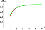
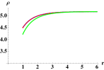
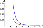
Figure 1: Asymptotic vortex solutions for dimension 2 condensation, charge density, and magnetic flux, respectively, where $\kappa=1$ is used. Both the blue line with $[\,a/b=-1$, $a/c=2\,]$ and the green line with $[\,a/b=1$, $a/c=6\,]$ correspond to repulsive interactions between vortices while the dashed red line with $[\,a/b=-1$, $a/c=6\,]$ results in attractive interactions.

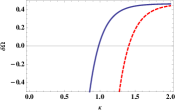
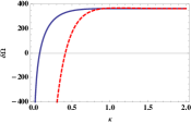
Figure 2: Effective interactions between vortices as a function of $\kappa$. With decreasing $\kappa$ the effective potential changes from repulsive to attractive. The nearest interaction was considered where $d_{L}=3$. Left: $T/T_{c}=0.907$, $b/a=-1$, $a/c=3$ (Blue Solid), and $a/c=10$ (Red Dashed). Right: $T/T_{c}=0.388$, $b/a=-1$, $a/c=3$ (Blue Solid), and $a/c=10$ (Red Dashed).

We classify our systems into four classes under the condition of $b/a<0$, depending on the density of U(1) charges and the ratio of $a/c$. First, we fix the density of U(1) charges, determining the chemical potential. We expect that the regime with $a/c\ll 1$ belongs to the type II superconductivity because the first term of the vortex interaction in Eq. (10) becomes larger than the second term, resulting in repulsive interactions. Physically, this relation implies strong supercurrents around the vortex core, consistent with the picture of type II. On the other hand, the regime with $a/c\gg 1$ will show that interactions between vortices change from repulsive when $\kappa\gg 1$ to attractive when $\kappa\ll 1$. Notice that $\kappa$ is introduced into the second term, reducing it with $\kappa\gg 1$ and enhancing it with $\kappa\ll 1$. Both $\mathcal{A}$ and $\mathcal{B}$ are positive definite, decreasing monotonically as we increase $\kappa$. We uncover that the regime with $b/a<0$ gives rise to $\mathcal{A}-\mathcal{B}>0$, allowing the possibility for the change of interactions. Fig. 2 confirms our expectation, that is, interactions between vortices become attractive when $\kappa<\kappa_{t}$, where $\kappa_{t}$ can be regarded as the tricritical point.

Next, we consider cases with a fixed $\kappa$. When $\kappa$ is rather large, it is difficult to find the tricritical point $\mu_{t}$, originating from smallness of the second term. In this respect it is better to start from a small enough $\kappa$. Then, the effective interaction is attractive when $\mu>\mu_{t}$ while it becomes repulsive when $\mu<\mu_{t}$. Figure 3 shows a surface of tricritical points in the space of $(\kappa,\mu/T)$ with a fixed $T$, $a/c>1$, and $b/a<0$, where effective interactions between vortices vanish exactly. The vortex interaction is attractive inside the ellipse while it is repulsive outside the ellipse. We claim that this ellipse serves a general criterion for the fluctuation-driven first-order superconducting transition in strongly coupled conformal field theories, possibly occurring in the vicinity of quantum criticality.

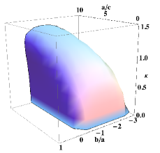
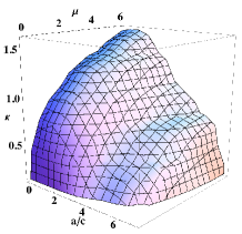
Figure 3: Tricritical surfaces in $(b/a,a/c,\kappa)$ with a fixed $\mu$ for the left panel and $(\mu,a/c,\kappa)$ with a fixed $b/a$ for the right panel, respectively, where vortices do not interact with each other. The interaction potential is attractive inside the ellipse while repulsive outside it.

In this study we try to answer how to classify strongly interacting field theories, considering the nature of the superconducting transition. The holographic superconductor model is our main ansatz as an effective low energy theory, expected to describe certain classes of strongly coupled conformal field theories. The effective interaction between vortices is our central object, allowing us to distinguish the type II superconductor from type I, where the former will show the second order transition while the latter will display the first order. As shown, an asymptotic solution for a single vortex configuration plays an essential role for the effective interaction. The effective interaction between vortices turns out to be a complicated function of both $\kappa$ and $\mu/T$, where the parameter $\kappa$ is introduced to play basically the same role as the Ginzburg-Landau parameter. We find a surface of tricritical points in the parameter space of $(\kappa,\mu/T)$, where the effective interaction vanishes, which separates the first order from the second order, proposed to be a general criterion in classifying quantum critical metals.

There are various unsolved questions in this direction. First of all, a possible topological term such as the axion term Axion_Vortex may play an important role in the vortex interaction. It can assign the U(1) charge to a vortex, modifying their interactions. We suspect the possibility of the BKT transition BKT , resulting from their Coulomb interactions due to the assigned U(1) charge, where $1/q^{2}$ in the momentum space becomes $\ln r$ in two space dimensions. In addition to this problem, the role of the pairing symmetry is not investigated, where non $s$-wave superconductivity arises in strongly interacting electrons QCP_Review1 . Furthermore, it should be studied the role of fermions in the vortex interaction.

We would like to thank T.Albash for providing us with details in his work. K.Kim would like to thank Ki-myeong Lee and Chanju Kim for helpful discussions. K.-S. Kim was supported by the National Research Foundation of Korea (NRF) grant funded by the Korea government (MEST) (No. 2010-0074542). Y.Kim acknowledges the Max Planck Society(MPG), the Korea Ministry of Education, Science, and Technology(MEST), Gyeongsangbuk-Do and Pohang City for the support of the Independent Junior Research Group at the Asia Pacific Center for Theoretical Physics(APCTP). K.Kim was supported by KRF-2007-313- C00150, WCU Grant No. R32-2008-000- 10130-0.

Appendix A Numerical analysis for Eq. (5)

We start with discussion about a uniform solution in the original holographic superconductor model [S. A. Hartnoll, C. P. Herzog, G. T. Horowitz, Phys. Rev. Lett. 101, 031601(2008)], where $Q_{t}^{s}(z)$ and $\eta^{s}(z)$ depend only on the $z$-coordinate. It is straightforward to derive equations of motion from Eq. (3)

$${\eta}^{\prime\prime}+\left(\frac{f^{\prime}}{f}-\frac{2}{z}\right){\eta}^{\prime}+\left(\frac{2}{z^{2}f}+\frac{\,{Q_{t}}^{2}}{f^{2}}\right)\eta=0,\qquad{{Q}_{t}}^{\prime\prime}-\frac{\eta^{2}}{z^{2}f}{Q}_{t}=0.$$ (11)

The regularity at horizon ($z=1$) gives the following conditions

$$Q_{t}(1)=0,\quad Q_{t}^{\prime}(1)=v,\quad Q_{t}^{\prime\prime}(1)=-\frac{u^{2}v}{3},\quad$$ (12)

$$\eta(1)=u,\quad\eta^{\prime}(1)=\frac{2}{3}u,\quad\eta^{\prime\prime}(1)=\frac{1}{2}u\left(-\frac{8}{9}-\frac{v^{2}}{9}\right).$$ (13)

Using the above conditions, one can find solutions in terms of $u$ and $v$, based on the shooting method. Near the boundary ($z=0$), the solutions behave such as

$$\eta(z)\sim O_{1}(u,v)z+O_{2}(u,v)z^{2}+\cdots,\qquad Q_{t}(z)\sim\mu(u,v)+\rho(u,v)z+\cdots.$$ (14)

When we are considering operators with dimension 1 or 2, we should constrain solutions with either $O_{2}=0$ or $O_{1}=0$, respectively. Therefore $u$ and $v$ are not independent but related with each other. As a result, the space of solutions becomes one dimensional, allowing us to take “$v$” as a parameter for the solution of the holographic superconducting state. In other words, $v$ controls either temperature or charge density of the system. According to the AdS/CFT dictionary, the total charge is given by $\mathcal{Q}\sim-\int d^{2}x\,\alpha\,Q_{t}^{\prime}(0)$. When $T=\frac{3\alpha}{4\pi}$ is fixed, the charge density varies as a function of $v$. If the charge density is fixed, temperature changes as a function of $v$. One can say a similar statement for the chemical potential, $\alpha\,Q_{t}(0)$. Inserting the uniform solution of $Q_{t}^{s}(z)$ and $\eta^{s}(z)$ into Eq. (5), we can solve them numerically.

Equation (5) has two parameters of $\kappa_{1}$ and $\kappa_{2}$. Performing the scaling as discussed in the manuscript, we obtain the following regularity conditions near the horizon for $A(z)$, $B(z)$ and $C(z)$,

$$A(1)=a,\quad A^{\prime}(1)=a\left(\frac{2}{3}+\frac{2\kappa^{2}}{3}\right),\quad A^{\prime\prime}(1)=-\frac{4a}{9}-\frac{buv}{9}-\frac{av^{2}}{18}+\frac{4a\kappa^{2}}{9}+\frac{2a\kappa^{4}}{9},$$ (15)

$$B(1)=0,\quad B^{\prime}(1)=b,\quad B^{\prime\prime}(1)=-\frac{2}{3}auv+\frac{1}{3}b\left(-u^{2}+2\kappa^{2}\right),$$ (16)

$$C(1)=c,\quad C^{\prime}(1)=c\left(\frac{1}{3}-\frac{u^{2}}{3}\right),\quad C^{\prime\prime}(1)=c\left(-\frac{5}{18}+\frac{u^{2}}{3}+\frac{u^{4}}{18}\right).$$ (17)

It is straightforward to see the scaling symmetries in Eq. (5). Equation for $C(z)$ remains invariant after scaling as $c\,\tilde{C}(z)$ with a parameter $c$. In this case $c=1$ is allowed due to the boundary condition in Eq. (A7). Equations for $A(z)$ and $B(z)$ also allow scaling, unchanged after $a\tilde{A}(z)$ and $a\tilde{B}(z)$. Therefore $b/a$ and $\kappa$ are only relevant parameters, governing equations for $A(z)$ and $B(z)$. As a result one may regard the asymptotic solution of the single vortex configuration as

$$s=a\tilde{A}\Bigl{(}v,\kappa,\frac{b}{a},z\Bigr{)}K_{0}\bigl{(}\sqrt{2}\kappa\bar{r}\bigr{)},\quad q_{t}=a\tilde{B}\Bigl{(}v,\kappa,\frac{b}{a},z\Bigr{)}K_{0}\bigl{(}\sqrt{2}\kappa\bar{r}\bigr{)},\quad q_{\theta}=c\,\tilde{C}(v,z)K_{1}(\bar{r})~{},$$ (18)

where $\bar{r}$ means a re-scaled coordinate with $\kappa_{2}$. We emphasize arguments in each function.

Appendix B Derivation of the variation for the grand potential

Inserting Eq. (6) into Eq. (3), we find the following linearized equations

$$\mathcal{D}^{2}\delta\eta-m^{2}\delta\eta-\delta\eta{Q^{v}_{\mu}}^{2}-2\eta^{v}Q^{v}_{\mu}\delta Q^{\mu}=0,$$ (19)

$$\mathcal{D}_{\mu}\delta B^{\mu\nu}-2\eta^{v}\delta\eta Q^{\nu}-{\eta^{v}}^{2}\delta Q^{\nu}=-\mathcal{D}_{\mu}\delta X^{\mu\nu},$$ (20)

proven to be valid near the center of a vortex. One can see that this approximation is reasonable only when $\delta\eta$ and $\delta Q_{t}$ are both larger than $\delta Q_{i}^{2}$ and smaller than $\eta^{v}$ and $Q_{t}^{v}$. The boundary of a Wigner-Seitz cell also satisfies these conditions. In this respect the linearized equations are valid not only near a vortex but also the boundary of the cell. This is a simple extension of the observation in L. Kramer, Phys. Rev. B 3, 3821 (1971).

Inserting the vortex solution [Eq. (6) with Eq. (8)] into the effective gravity action [Eq. (1)] and expanding the action to the second order, we obtain the following expression for the change of the grand potential in a cell

$$\delta\Omega=\frac{1}{T}\int_{\hat{i}}dzd^{2}x\partial_{\mu}\left\{\sqrt{-g}\left[\delta\eta\mathcal{D}^{\mu}\Bigl{(}\eta^{v}+\frac{1}{2}\delta\eta\Bigr{)}+\delta Q_{\nu}\Bigl{(}B^{v\mu\nu}+\frac{1}{2}\delta B^{\mu\nu}\Bigr{)}\right]\right\},$$ (21)

where Eqs. (B1) and (B2) are utilized. In this derivation we need to worry about singular parts from $X_{\mu\nu}$. $\delta X_{\mu\nu}$ vanishes identically because the singularity appears completely outside the cell $\hat{i}$. The only term that we have to concern is $\delta B_{\mu\nu}X^{\mu\nu}$, however this turns out to vanish when we are considering the configuration of $\delta B_{\mu\nu}=0$ at the origin of the cell.

Changing Eq. (21) into surface integrals, we have three kinds of boundaries. The first is the boundary at the horizon $(z=1)$ of the black hole and the second is that of the AdS space $(z=0)$. The last is the boundary of the Wigner-Seitz cell. The first contribution vanishes identically thanks to regularity conditions at the horizon. For the $z=0$ boundary, the contribution must be considered carefully. Actually, this contribution could be important, when a distance between vortices is comparable to a size of a vortex. However, we are taking the dilute gas limit, thus the variation from the single vortex solution will be concentrated on boundaries of Wigner-Seitz cells.

The surface integral for $z=0$ is given as follows

$$\delta\Omega_{z=0}=\frac{1}{T}\int_{\hat{i}}d^{2}x\sqrt{-g}\left[\delta\eta\nabla^{z}\Bigl{(}\eta^{v}+\frac{1}{2}\delta\eta\Bigr{)}+\delta Q_{\nu}\Bigl{(}B^{v\,z\nu}+\frac{1}{2}\delta B^{z\nu}\Bigr{)}\right]_{z=0}.$$ (22)

In the dilute limit $\delta\eta$ and $\delta Q_{\mu}$ have nonzero values only near the boundary of a cell. Thus, the integration range is effectively small. As positions of vortices are far from each other, this contribution almost vanishes and it is much smaller than the third contribution given by the integration along the $z$ direction at the boundary of Wigner-Seitz cells. This dilute approximation serves the validity of our calculation. Therefore, our correction of the grand potential is well approximated as

$$\delta\Omega\sim\frac{1}{T}\int_{0}^{1}dz\oint_{\hat{i}}dl\hat{n}_{i}\sqrt{-g}\left[\delta\eta\nabla^{i}\Bigl{(}\eta^{v}+\frac{1}{2}\delta\eta\Bigr{)}+\delta Q_{\nu}\Bigl{(}B^{v\,i\nu}+\frac{1}{2}\delta B^{i\nu}\Bigr{)}\right],$$ (23)

where $\hat{n}_{i}$ is a unit vector orthogonal to the boundary of the Wigner-Seitz cell. This leads to Eq. (9).

Appendix C Derivation of Eq. (9)

In this section we will derive the following formulae

$$\sum_{i\neq 0}\oint dl\,\hat{n}\cdot K_{0}(|r-r_{i}|)\hat{\theta}(\vec{r}-\vec{r}_{i})\times\nabla\times\Bigl{(}K_{0}(r)\hat{\theta}+\frac{1}{2}\sum_{j\neq 0,i}K_{0}(|r-r_{j}|)\hat{\theta}(\vec{r}-\vec{r}_{j})\Bigr{)}=\pi\sum_{i\neq 0}K_{0}(|\vec{r}_{i}|),$$ (24)

$$\sum_{i\neq 0}\oint dl\,\hat{n}\cdot K_{0}(|r-r_{i}|)\nabla\Bigl{(}K_{0}(r)+\frac{1}{2}\sum_{j\neq 0,i}K_{0}(|r-r_{j}|)\Bigr{)}=-\pi\sum_{i\neq 0}K_{0}(|\vec{r}_{i}|).$$ (25)

For convenience, we define a fictitious coordinate $w$ and vector fields, $h_{i}(\vec{r})\equiv K_{0}(|r-r_{i}|)\hat{w}$, where $r_{i}$ is a center of a lattice. Then, the above equations can be written as follows

$$F1\equiv\sum_{i\neq 0}\oint d\vec{S}\cdot\left\{\Bigl{(}h_{0}+\frac{1}{2}\sum_{j\neq 0,i}h_{j}\Bigr{)}\times\Bigl{(}\nabla\times h_{i}\Bigr{)}\right\}=\pi\sum_{i\neq 0}h_{i}\cdot\hat{w},$$ (26)

$$F2\equiv\sum_{i\neq 0}\oint d\vec{S}\cdot h_{i}\times\nabla\times\Bigl{(}h_{0}+\frac{1}{2}\sum_{j\neq 0,i}h_{j}\Bigr{)}=-\pi\sum_{i\neq 0}h_{i}\cdot\hat{w}~{}~{},$$ (27)

where $d\vec{S}$ is an area element orthogonal to the boundary surface of a cell, i.e, $d\vec{S}=dl~{}dw~{}\hat{n}$.

Using the divergence theorem and taking integration by parts, one can rearrange $F1$ into

$$F1 = \sum_{i\neq 0}\int d^{3}x\Biggl{\{}\nabla\times\Bigl{(}h_{0}+\frac{1}{2}\sum_{j\neq 0,i}h_{j}\Bigl{)}\cdot(\nabla\times h_{i})-\Bigl{(}h_{0}+\frac{1}{2}\sum_{j\neq 0,i}h_{j}\Bigl{)}\cdot(\nabla\times\nabla\times h_{i})\Biggr{\}}$$ (28)

$$= \sum_{i\neq 0}\int d^{3}x\Biggl{\{}\nabla\times\Bigl{(}h_{0}+\frac{1}{2}\sum_{j\neq 0,i}h_{j}\Bigl{)}\cdot(\nabla\times h_{i})+h_{i}\cdot\Bigl{[}2\pi\delta^{2}(r)\hat{w}-\nabla\times\nabla\times\Bigl{(}h_{0}+\frac{1}{2}\sum_{j\neq 0,i}h_{j}\Bigr{)}\Bigr{]}\Biggr{\}}$$

$$= 2\pi\sum_{i\neq 0}h_{i}(0)+\sum_{i\neq 0}\oint d\vec{S}\cdot\Biggl{\{}h_{i}\times\nabla\times\Bigl{(}h_{0}+\frac{1}{2}\sum_{j\neq 0,i}h_{j}\Bigr{)}\Biggr{\}}~{}~{},$$

where we have used $\nabla\times\nabla\times h_{i}+h_{i}=2\pi\delta^{2}(\vec{r}-\vec{r}_{i})\hat{w}$ with some algebra. Actually, the second term in the last is equal to $-F1$. In order to show this, we consider the following combination,

$$\sum_{i\neq 0}\oint d\vec{S}\cdot\Biggl{\{}\Bigl{(}h_{0}+\frac{1}{2}\sum_{j\neq 0,i}h_{j}\Bigr{)}\times\nabla\times h_{i}\Biggr{\}}+\sum_{i\neq 0}\oint d\vec{S}\cdot\Biggl{\{}h_{i}\times\nabla\times\Bigl{(}h_{0}+\frac{1}{2}\sum_{j\neq 0,i}h_{j}\Bigr{)}\Biggr{\}}$$

$$\quad=\oint d\vec{S}\cdot\nabla\sum_{i\neq 0}h_{0}\cdot\Bigl{(}h_{0}+\frac{1}{2}\sum_{j\neq 0,i}h_{j}\Bigr{)}$$

$$\quad=\oint d\vec{S}\cdot\nabla\Biggl{\{}h_{k}\cdot h_{0}+(h_{0}+h_{k})\cdot\sum_{i\neq 0,k}h_{i}+\frac{1}{2}\sum_{i\neq 0,k}h_{i}\cdot\!\sum_{j\neq 0,k,i}h_{j}\Biggr{\}},$$ (29)

where $k$ means one of other vortices. The integrand is symmetric under interchange of $h_{0}$ and $h_{k}$. Now, we may take $\vec{r}_{k}$ as one of the nearest neighbor. Then, the symmetry means that the integrand is a vector whose direction is along the boundary surface of the cell. Thus, the above combination should vanish, leading us to conclude that $F1=\pi\sum_{i\neq 0}h_{i}(0)\cdot\hat{w}$. This argument is in parallel with that in L. Kramer, Phys. Rev. B 3, 3821 (1971). For $F2$, one can see that $F2=-F1$ from Eq. (C). This completes our derivation.

References

• (1) L. Kramer, Phys. Rev. B 3, 3821 (1971).
• (2) L. Jacobs and C. Rebbi, Phys. Rev. B 19, 4486 (1979).
• (3) S. Mo, J. Hove, and A. Sudbo, Phys. Rev. B 65, 104501 (2002); F. Mohamed, M. Troyer, G. Blatter, and I. Lukyanchuk, Phys. Rev. B 65, 224504 (2002); A. Chaves, F. M. Peeters, G. A. Farias, and M. Milosevic, Phys. Rev. B 83, 054516 (2011).
• (4) F. S. Nogueira and H. Kleinert, arXiv:cond-mat/0303485, to appear in the World Scientific review volume โ€Order, Disorder, and Criticalityโ€, Edited by Y. Holovatch.
• (5) B. I. Halperin, T. C. Lubensky, and S.-K. Ma, Phys. Rev. Lett. 32, 292 (1974); J.-H. Chen, T. C. Lubensky, and D. R. Nelson, Phys. Rev. B 17, 4274 (1978).
• (6) S. Coleman and E. Weinberg, Phys. Rev. D 7, 1888 (1983).
• (7) H. v. Lohneysen, A. Rosch, M. Vojta, and P. Wolfle, Rev. Mod. Phys. 79, 1015 (2007).
• (8) D. Belitz, T. R. Kirkpatrick, and T. Vojta, Rev. Mod. Phys. 77, 579 (2005).
• (9) J. Rech, C. Pรฉpin, and A. V. Chubukov, Phys. Rev. B 74, 195126 (2006).
• (10) Sung-Sik Lee, Phys. Rev. B 80, 165102 (2009).
• (11) Max A. Metlitski and S. Sachdev, Phys. Rev. B 82, 075127 (2010).
• (12) J. M. Maldacena, Adv. Theor. Math. Phys. 2, 231 (1998); Int. J. Theor. Phys. 38, 1113 (1999).
• (13) E. Witten, Adv. Theor. Math. Phys. 2, 253 (1998); S. S. Gubser, I. R. Klebanov, and A. M. Polyakov, Phys. Lett. B 428, 105 (1998).
• (14) O. Aharony, S.S. Gubser, J. Maldacena, H. Ooguri, Y. Oz, Phys. Rept. 323, 183 (2000).
• (15) For reviews, see J.ย Erdmenger, N.ย Evans, I.ย Kirsch and E.ย Threlfall, Eur. Phys. J. A 35, 81 (2008); J. McGreevy, Adv. High Energy Phys. 2010, 723105 (2010); J. Casalderrey-Solana, H. Liu, D. Mateos, K. Rajagopal, and U. A. Wiedemann, arXiv:1101.0618 [hep-th].
• (16) C. P. Herzog, P. Kovtun, S. Sachdev, and D. T. Son, Phys. Rev. D 75, 085020 (2007); S. A. Hartnoll, P. K. Kovtun, M. Muller, and S. Sachdev, Phys. Rev. B 76, 144502 (2007).
• (17) Sung-Sik Lee, Phys. Rev. D 79, 086006 (2009); M. Cubrovic, J. Zaanen, and K. Schalm, Science 24, 439 (2009).
• (18) T. Faulkner, N. Iqbal, H. Liu, J. McGreevy, and D. Vegh Science 27, 1043 (2010).
• (19) S. S. Gubser, Phys. Rev. D 78, 065034 (2008).
• (20) S. A. Hartnoll, C. P. Herzog, G. T. Horowitz, Phys. Rev. Lett. 101, 031601(2008).
• (21) Vortex solutions in the holographic superconductor model can be found in T. Albash, C. V. Johnson Phys. Rev. D 80, 126009 (2009); G. Tallarita, S. Thomas, JHEP 1012 090 (2010); V. Keranen, E. Keski-Vakkuri, S. Nowling, K. P. Yogendran, Phys. Rev. D 81, 126012 (2010); K. Maeda, M. Natsuume, T. Okamura, Phys. Rev. D 81, 026002 (2010); M. Montull, A. Pomarol, P. J. Silva, arXiv:0906.2396.
• (22) See appendices.
• (23) We used โˆ‘iโ‰ 0hiโ‹…z^=โˆ‘iโ‰ 0โˆฎdโ€‹Sโ†’ฯ€โ‹…(h0+12โ€‹โˆ‘jโ‰ 0,ihj)ร—(โˆ‡ร—hi)=โˆ’โˆ‘iโ‰ 0โˆฎdโ€‹Sโ†’ฯ€โ‹…hiร—โˆ‡ร—(h0+12โ€‹โˆ‘jโ‰ 0,ihj)subscript๐‘–0โ‹…subscriptโ„Ž๐‘–^๐‘งsubscript๐‘–0contour-integralโ‹…๐‘‘โ†’๐‘†๐œ‹subscriptโ„Ž012subscript๐‘—0๐‘–subscriptโ„Ž๐‘—โˆ‡subscriptโ„Ž๐‘–subscript๐‘–0contour-integralโ‹…๐‘‘โ†’๐‘†๐œ‹subscriptโ„Ž๐‘–โˆ‡subscriptโ„Ž012subscript๐‘—0๐‘–subscriptโ„Ž๐‘—\sum_{i\neq 0}h_{i}\!\cdot\!\hat{z}=\sum_{i\neq 0}\oint\!\frac{d\vec{S}}{\pi}\!\cdot\!\Bigl{(}h_{0}+\frac{1}{2}\!\sum_{j\neq 0,i}\!h_{j}\Bigr{)}\times\left(\nabla\times h_{i}\right)=-\sum_{i\neq 0}\oint\!\frac{d\vec{S}}{\pi}\!\cdot\!h_{i}\times\nabla\times\Bigl{(}h_{0}+\frac{1}{2}\sum_{j\neq 0,i}\!h_{j}\Bigr{)}, where $h_{i}\equiv K_{0}(|\vec{x}-\vec{x}_{\hat{i}}|)\hat{z}$. See appendix C.
• (24) F. Chandelier, Y. Georgelin, M. Lassaut, T. Masson, and J. C. Wallet, Phys. Rev. D 70, 065016 (2004).
• (25) V. L. Berezinskii, Sov. Phys. JETP 32, 493 (1971); J. M. Kosterlitz and D. J. Thouless, J. Phys. C 6, 1181 (1973).