Characterization of Random Linear Network Coding with Application to Broadcast Optimization in Intermittently Connected Networks

Abstract

We address the problem of optimizing the throughput of network coded traffic in mobile networks operating in challenging environments where connectivity is intermittent and locally available memory space is limited. Random linear network coding (RLNC) is shown to be equivalent (across all possible initial conditions) to a random message selection strategy where nodes are able to exchange buffer occupancy information during contacts. This result creates the premises for a tractable analysis of RLNC packet spread, which is in turn used for enhancing its throughput under broadcast. By exploiting the similarity between channel coding and RLNC in intermittently connected networks, we show that quite surprisingly, network coding, when not used properly, is still significantly underutilizing network resources. We propose an enhanced forwarding protocol that increases considerably the throughput for practical cases, with negligible additional delay.

I Introduction

The paper focuses on improving throughput in intermittently connected networks while maintaining low delivery delays. Intermittently connected networks (or DTNs – disruption tolerant networks) are networks of very mobile, power- and memory-constrained devices where connectivity is sporadic. This is the model of choice for wireless networks operating in challenging conditions (networks of UAVs, disaster relief scenarios, etc.). As traditional routing approaches cannot be applied in this case (little is known in advance about future connectivity), the literature has developed opportunistic (epidemic) forwarding protocols that replicate packets to multiple relay nodes in order to optimize the delivery delay and/or the chance that packets get delivered to the destination(s) [1]. Increasing throughput, while keeping low delay, is a problem of practical interest as it would enable nodes to receive more information per time unit, with almost the same delay. RLNC has emerged recently as a promising approach for such applications. It ameliorates the transmission by introducing the diversity of multiple independent combinations in the epidemic forwarding. Nevertheless, analyzing and optimizing RLNC for DTNs is difficult[2]. We prove that RLNC in DTNs is in fact equivalent to a forwarding algorithm not employing network coding, which is much easier to analyze. Using this equivalence, we show that RLNC still produces too many redundant packets during contacts, thereby underutilizing network resources (inter-contact times and consequently buffer space). Our study shows that transmissions of a backlogged source can be conveniently pipelined even though no feedback from destinations is available such that significant throughput gains can be attained with negligible additional delay. Based on these observations, we design and evaluate a forwarding protocol with reduced buffer and energy requirements (less mobility required for collecting the same number packets).

Related work: In their seminal paper, Deb et al.[3] offer an in-depth analysis of random linear network coding (RLNC) for networks with intermittent contacts. Numerous studies have built upon these results, extending them to the case of DTNs[4, 5, 6]; RLNC is used to improve the average delivery ratio within a given time unit. Our work is motivated by the observation that these studies extend the conclusions of [3] past the assumptions under which those results have been obtained, such that they do not hold anymore. In particular, all protocols for optimizing throughput or delays in DTNs break the initial condition assumption (messages do not have equal initial spread), which leads to significant throughput loss. Both Lin et al.[6] and Altman et al.[7] (which studies network coding and Reed-Solomon codes in two-hop DTNs) note the similarity between channel coding and data transmission in DTNs. We study the implications of this analogy on the aforementioned initial condition assumption.

II Network Models

The network model is similar to the one used in [2]. The network consists of $N$ mobile nodes with the same radio range and buffer space $B$. We consider that a wireless link (contact) is established between two nodes when they are in each others’ radio range. All contacts are bidirectional. Their duration is considered to be negligible with respect to the inter-contact times, but sufficient enough to allow the transmission of one packet in each direction. We consider mainly the case of a backlogged source broadcasting data to the entire network and then extend the conclusions to multi- and unicast. The source aims at maximizing the average throughput at destinations. We consider a mobility model with exponential inter-contact times of parameter $\lambda$, which has been validated for a wide spectrum of mobility scenarios[8]. Our analysis is however not constrained to this type of mobility.

The backlogged source is considered to have at least $\nu\in\mathbb{N}$ packets in its buffer. These packets will be called hereafter variables and represent original (not coded) source-generated packets. Out of them, the source selects every time a set of $\nu$ oldest packets to be transmitted in the network. When the transmission of the $\nu$ packets is considered completed (after a fixed time, TTL, set as a function of $N$), they are deleted by all nodes, the source selects the next $\nu$ packets and repeats the operation. Minimizing the time to delivery and the probability that not all nodes have decoded the content are desirable.

All nodes implement random linear network coding over a finite field $GF({2^{k}})$. The source is assumed to send to nodes that it encounters coded packets (one such packet/contact). Coded packets are elements in the set of $\nu$ independent linear combinations of $\nu$ variables (set called packet batch), where coefficients are randomly selected from $GF({2^{k}})$. Note that $\nu\leq B$ and the buffer occupancy is described by the number of independent linear combinations present in a node’s buffer. Packets have size $K$ (a multiple of $k$) and are treated as vectors of values from $GF({2^{k}})$. During a contact, nodes scale each vector (coded packet) in their buffers with randomly selected elements from $GF({2^{k}})$ and adds them, thereby creating a new network coded packet, which is sent to the other node. A node is able to decode all variables only when it has received $\nu$ independent linear combinations. We say that a coded packet received by a node is innovative if it increases the rank of the equation system formed by coded packets in that node’s buffer. A contact is efficient iff at least one innovative packet is transferred. We are analyzing two protocols: one in which relay nodes send random linear combinations of coded packets stored in their buffer during contacts (as described above) and the other where nodes compare their buffers and only forward to each other (coded) packets selected uniformly at random among those not contained by the other. The two protocols are denoted by $\Gamma$ (true RLNC) and $\Delta$ (a type of random message selection), respectively. RLNC schemes transport along with packets the random coefficients as well as the identities of original variables combined in the coded packets, providing therefore a distributed solution[9, 10]. It can be proven that the overhead of storing and transporting these random coefficients is small. Note that $\Delta$ can also be used with variables as packets (instead of coded packets), as relays do not perform network coding, thus eliminating coefficient overhead. $\Gamma$ and $\Delta$ are similar to E-NCP, E-RP[6].

III Main Results

III-A Random Message Selection with Feedback vs. RLNC

The following result shows that the operation of random message selection with buffer feedback during contacts ($\Delta$) is almost identical to true RLNC ($\Gamma$). Thus, results for $\Delta$ apply to $\Gamma$ and vice versa. The equivalence uncovered by this theorem can be used for designing optimal distributed network coding protocols for intermittently-connected networks, initially under the more tractable $\Delta$, then applied to $\Gamma$. $\Delta$ relies on nodes exchanging information about the list of packets in buffers, during contacts. Should this capability not be available, $\Gamma$-type RLNC offers the distributed counterpart.

Theorem III.1

Given identical mobility and initial conditions (set of packets already disseminated by the source in the network and which are prepared to start the epidemic network spread), an arbitrarily-selected contact between two nodes $A$ and $B$ at time $t$ will have approximately the same probability that $A$ delivers a novel packet to $B$, under both $\Gamma$ and $\Delta$.

Proof:

We use the following notation: for a node $w$, $S^{-}_{w}$ and $S^{+}_{w}$ designate the subspace spanned by the coded packets belonging to this node’s buffer, before and after a contact with another node $v$, respectively. It is thus easy to infer[3] that:

$$Pr[S^{+}_{w}\nsubseteq S^{-}_{u}|S^{-}_{w}\subseteq S^{-}_{u},S^{-}_{v}\nsubseteq S^{-}_{u}] \geq 1-\frac{1}{q}$$ (1)

$$Pr[dim(S^{+}_{w})>dim(S^{-}_{w})|S^{-}_{v}\nsubseteq S^{-}_{w}] \geq 1-\frac{1}{q}$$ (2)

where $q=|GF(2^{k})|$ and $u$ can be any other node. The two probabilities describe the way a node $w$ acquires new degrees of freedom in its buffer under RLNC with $\Gamma$-type forwarding. Each of these probabilities is equal to $1$ for $\Delta$-type forwarding, so eq. (1) and (2) continue to be true even for $\Delta$. If we consider the case of a very large $q$ ($q\rightarrow+\infty$), then $\Gamma$ and $\Delta$ become identical. For known mobility and known initial packet distribution, we can construct a DTMC to capture the packet propagation. A state contains an array of size $N$ and an element of this array at index $i$ has to store the list of degrees of freedom acquired by node $i$ until that time step. There are $N$ degrees of freedom under both $\Gamma$ and $\Delta$. Consider a contact between nodes $A$ and $B$, where we analyze only the transmission from $A$ to $B$. From eq. (1), (2) this transmission is successful iff node $A$’s buffer has one degree of freedom not available to $B$. In both $\Gamma$ and $\Delta$ this degree of freedom is selected uniformly at random from those available to $A$ and not available to $B$. Thus, the transition probabilities are the same for both DTMCs and the two protocols behave identically. In a more realistic setting when $q$ is finite, RLNC with $\Gamma$ will in fact slightly underperform $\Delta$, because the probabilities in eq. (1), (2) will be $1$ for $\Delta$ and $\geq 1-\frac{1}{q}$ for $\Gamma$.

To prove rigorously that the uniform selection of degrees of freedom (dimensions) leads to similar behavior of $\Gamma$ and $\Delta$, we have to postulate the following elementary theorem, known from linear algebra, presented here without proof:

Every $n$-dimensional vector space $V$ over some finite field $F$ is isomorphic to $F^{n}$. If $v_{1},v_{2},v_{3},\ldots,v_{n}$ is a basis of $V$, then the mapping $\phi:F^{n}\rightarrow V$ : $(a_{1},\ldots,a_{n})\mapsto\sum_{k=1}^{n}a_{k}v_{k}$ is an isomorphism.

Observation: Since the choice of basis for V is not unique (there are many possibilities) $\Rightarrow$ the above isomorphism is also not unique. In fact, we can construct many such isomorphisms.

Final steps: We need this isomorphism simply because tracking the evolution of vector spaces (that is, node buffers) during the packet spread process is very challenging. Such isomorphisms offer an easy way to label buffers in a consistent manner. In particular, we are interested in mapping each buffer to a subset of the base $\{p_{1},\ldots,p_{\nu}\}$, where $p_{1},\ldots,p_{\nu}$ are the initial packets at source. We regard each buffer as a subspace/subset of the $\nu$-dimensional vector space. Each such buffer/subspace is generated by the vectors/packets present in it. Note that the labelling will be performed for every node, at will hold at every step of the packet spread. However, a final point needs to be discussed. One has to observe that we cannot simply map all $k$-dimensional subspaces to the same set of $k$ vectors of the base (actually, to the subspace that they generate). This is simply because then all buffers will look identical after applying the isomorphism. Based on the fact that every intersection of subspaces is also a subspace, we can build the mappings/labellings for each node in a way that can prevent this problem. To this end, we specify a hard constraint requiring that the intersection of subspaces be respected even after applying the isomorphism. This can be translate as follows: the intersection of any number of subspaces (buffers) has to be a subspace of the same dimension in the original version and after applying the isomorphism. This is effectively the final step of our proof. The attentive reader will have already noticed that instead of working with coded packets, we have mapped our buffers to sets of original packets, thus effectively equating $\Gamma$ to $\Delta$. ∎

III-B Finding Optimal Spread Ratios

We analyze how the number of coded packet copies influences the instant throughput of broadcast under $\Delta$-type forwarding and extend the result to $\Gamma$ forwarding, uni- and multicast. For our mobility model, if coded packets have each the same number of copies in the network at the beginning of the forwarding, then, for an arbitrary $k$, $Pr[$node $\ell$ has a copy of coded packet $p_{k}]=\zeta_{k}=ct.,(\forall)\ell$. $m_{p_{i}}(t)$ is the number of copies of $p_{i}$ contained by network at time $t$ (not counting the source), and $\rho_{p_{i}}(t)=\frac{m_{p_{i}}(t)}{N-1}$ is the correspondent instant density. We seek to find the relation between $\rho_{p_{i}}(t),i=\overline{1,\nu}$ that maximizes the instantaneous throughput. For this, we analyze the efficiency of each node’s first contact after instant $t$, arbitrarily chosen. For tractability, we first look at the case when each relay node contains exactly one coded packet at time $t$ and generalize afterwards. In this case, $\sum\limits_{i=1}^{\nu}m_{p_{i}}(t)=N-1,\sum\limits_{i=1}^{\nu}\rho_{p_{i}}(t)=1$. We exclude w.l.o.g. the source as its contacts are efficient by definition anyway. If ${\cal A}_{p_{i}}^{(t)}$ is the set of nodes (without the source) containing a copy of coded packet $p_{i}$ at time $t$, $|{\cal A}_{p_{i}}^{(t)}|=m_{p_{i}}(t)$, $(\forall)i=\overline{1,\nu}\Rightarrow\bigcup\limits_{i=1}^{\nu}{\cal A}_{p_{i}}^{(t)}={\cal N}-\{s\},{\cal A}_{p_{i}}^{(t)}\cap{\cal A}_{p_{j}}^{(t)}=\emptyset,(\forall)i\neq j$, where ${\cal N}-\{s\}$ is the set of all nodes, without the source. For an arbitrary $\ell\in{\cal A}_{p_{i}}^{(t)},Pr[$next contact of $\ell$ is inefficient$]=\rho_{p_{i}}(t)-\frac{1}{N-1}$ (efficient with probability $1-\rho_{p_{i}}(t)+\frac{1}{N-1}$), meaning that $\ell$ has met another node from the same set, no data transfer occurred and the waiting time preceding the contact had been wasted.

We are interested in maximizing throughput (maximizing the expected number of efficient first contacts of each node after instant $t$). Therefore, under $\sum\limits_{j=1}^{\nu}\rho_{p_{j}}(t)=1$ we maximize

$$f(\rho_{p_{1}}(t),\ldots,\rho_{p_{\nu}}(t)) = \sum\limits_{k=1}^{\nu}\sum\limits_{\ell\in{\cal A}_{k}^{(t)}}(1-\rho_{p_{k}}(t))=$$ (3)

$$=\sum\limits_{k=1}^{\nu}m_{p_{k}}(1-\rho_{p_{k}}) = (N-1)\cdot\sum\limits_{k=1}^{\nu}\rho_{p_{k}}(1-\rho_{p_{k}})$$ (4)

Using Lagrange multipliers,

$$\Lambda(\rho_{p_{1}}(t),\ldots,\rho_{p_{\nu}}(t),\lambda_{sol})=f(\rho_{p_{1}}(t),\ldots,\rho_{p_{\nu}}(t))+$$ (5)

$$\lambda_{sol}\cdot(\sum\limits_{k=1}^{\nu}\rho_{p_{k}}(t)-1)\Rightarrow\frac{\partial\Lambda}{\partial\rho_{p_{k}}}=(N-1)\cdot(1-2\rho_{p_{k}})$$ (6)

$$+\lambda_{sol}=0\Rightarrow\lambda_{sol}=\frac{2(N-1)}{\nu}-(N-1)$$ (7)

Replacing $\lambda_{sol}$ we find that $\rho_{p_{1}}(t)=\ldots=\rho_{p_{\nu}}(t)\triangleq\rho(t)=\frac{1}{\nu}$. Thus, all densities should be equal at instant $t$. The generalization for the case of more (or less) than $1$ packet/node on average ($\sum\limits_{j=1}^{\nu}\rho_{p_{j}}(t)=c,c\geq 0$) is provided by

Theorem III.2

The following condition is necessary for maximizing throughput of a batch of $\nu$ coded packets in a DTN with $\Delta$-type forwarding: $\rho_{p_{1}}(t)=\rho_{p_{2}}(t)=\rho_{p_{3}}(t)=\ldots=\rho_{p_{\nu}}(t)\triangleq\rho(t),(\forall)t$. In other words, regardless of the buffer occupancy level, packet densities should be roughly equal to ensure maximal throughput.

Proof:

For each node $\ell$ define the concept of entire buffer packet as being the indicator function $1_{\ell}:\{p_{1},p_{2},p_{3},\ldots,p_{\nu}\}\rightarrow\{0,1\},1_{\ell}(p_{k})=1\Leftrightarrow$ the buffer of $\ell$ contains coded packet $p_{k}$. A contact between $\ell,\aleph\in{\cal N}$ is efficient $\Leftrightarrow 1_{\ell}\neq 1_{\aleph}$. Using the above argument for entire buffer packets we check that $\sum\limits_{{\ell}\in{\cal N}-\{s\}}\rho_{1_{\ell}}=1$ and therefore $\rho_{1_{\ell}}(t)=\rho_{buf}(t)=ct.,(\forall)\ell\in{\cal N}-\{s\}$ is necessary for throughput maximization. From this set of equalities at time $t$, considering an arbitrarily chosen but fixed entire buffer packet $1_{\aleph}\Rightarrow Pr[\ell\in{\cal A}_{1_{\aleph}}^{(t)}]=Pr[1_{\ell}(p_{1})=1_{\aleph}(p_{1})]\cdot Pr[1_{\ell}(p_{2})=1_{\aleph}(p_{2})]\cdot Pr[1_{\ell}(p_{1})=1_{\aleph}(p_{1})]\cdot\ldots\cdot Pr[1_{\ell}(p_{\nu})=1_{\aleph}(p_{\nu})]=\rho_{buf}(t)=ct.,(\forall)\ell\in{\cal N}-\{s\}$. But since none of the buffers is yet full ($\max_{{\ell}\in{\cal N}-\{s\}}|1_{\ell}|=\kappa<N$, $|1_{\ell}|=\kappa_{\ell}$ – $\ell$’s buffer occupancy) $\Rightarrow$ $Pr[1_{\ell}(p_{i_{1}})=1]\cdot Pr[1_{\ell}(p_{i_{2}})=1]\cdot Pr[1_{\ell}(p_{i_{3}})=1]\cdot\ldots\cdot Pr[1_{\ell}(p_{i_{\kappa_{\ell}}})=1]=\Omega=ct.,i_{1},i_{2},i_{3},...,i_{\kappa_{\ell}}=\overline{1,\nu},(\forall)\ell\in{\cal N}-\{s\}$. This is an equation system with $N-1$ product equations and $\nu\leq B\leq N$ unknowns, where each probability is known to be strictly positive. By equalizing equations with the same number of factors, we obtain that with high probability $Pr[1_{\ell}(p_{1})=1]=Pr[1_{\ell}(p_{2})=1]=Pr[1_{\ell}(p_{3})=1]=\ldots=Pr[1_{\ell}(p_{\nu})=1]=ct.,(\forall)\ell\in{\cal N}-\{s\}$, which means that coded packets should have equal spreads. ∎

Remark: The same condition is necessary for providing optimal throughput also for unicast and multicast. This is because each node will deliver a packet to the target(s) with equal probability.

III-C Impact of Packet Counts on Contact Efficiency

In this paragraph we explain why the assumption of equal packet spread cannot be taken for granted and demonstrate its performance impact. We define the entropy of relative (normalized) coded packet densities at time instant $t$ as $H(\rho^{\prime}(t))=\sum\limits_{k=1}^{\nu}\rho^{\prime}_{p_{k}}(t)\cdot\log_{\nu}(\frac{1}{\rho^{\prime}_{p_{k}}(t)})$, where $\rho^{\prime}(t)=(\rho^{\prime}_{p_{1}}(t),\rho^{\prime}_{p_{2}}(t),\rho^{\prime}_{p_{3}}(t),\ldots,\rho^{\prime}_{p_{\nu}}(t))$ and $\rho^{\prime}_{p_{k}}(t)\in[0,1]$ are the normalized counterparts of $\rho_{p_{k}}(t),(\forall)k=\overline{1,\nu}$. The entropy is close to $1$ iff network coded packets have similar instant densities in the network. The entropy allows us to quantify the discrepancy between densities through a scalar. We analyze the evolution with time of $H(\rho^{\prime}(t))$ and use as an example a network with $N=100$ nodes, $B=11$, $\lambda=0.005$. In Fig. 1(a)-1(b) we show how the entropy evolves over time using three representative mobility realizations that run until all destinations decode the data, for the following protocols:

• A benchmark $\Delta$-type protocol: the source transmits a batch of $11$ coded packets continuously until all destination nodes have decoded the data. No specific measure is taken to maintain equal densities;

• Another $\Delta$-type protocol with a batch of $10$ coded packets, each placed in a separate node before the spread is triggered. The source continues transmitting coded packets to non-full nodes;

• Similar to 2., with the exception that after distributing the initial copies and triggering their spread, the source stops disseminating data.

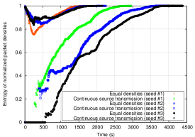
(a) Protocol 1 (continuous source transmission) vs. Protocol 2. (equal densities)

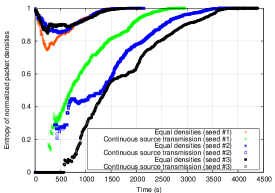
(b) Protocol 1 (continuous source transmission) vs. Protocol 3. (equal densities)

Figure 1: Comparison of instantaneous entropies of normalized network coded packet densities for a network of $100$ nodes

Remarks: There are a number of observations, which hold in general (also for $\Gamma$). Firstly, high entropies are conserved by exponential inter-contact times. Secondly, the delay of protocols 2. and 3. is always almost identical, meaning that the source intervention does not improve the throughput anymore and that high entropy should be sufficient for maximizing throughput. Thirdly, when the source injects packets in a greedy manner (strategy commonly considered to yield minimal delay[6]), the entropy drops significantly, impacting overall contact efficiency.

IV Improved Forwarding Protocol

We define the seeding phase of a transmission as the time interval used by source to place $\nu$ independent coded packets each on a distinct relay node, for a batch of $\nu$ variables. The time needed for this operation is a random variable $T^{s}_{n}$, where $n\in\mathbb{N}$ is the identifier of the packet batch (or $T^{s}$ when we do not refer to a specific $n$). Similarly, we define the propagation phase of the transmission as the interval in which the independent coded packets are forwarded epidemically in the network; this step finishes when all destination nodes have successfully decoded the packets. The time needed for the propagation phase of batch $n$ is another random variable, $T^{p}_{n}$ (identically distributed as $T^{p}$). For every packet batch, the propagation phase takes place immediately after the seeding phase. The key idea is that the seeding phase of packet batch $n+1$ can be performed in parallel with the propagation phase of the packet batch $n$. To accomplish this, we need to ensure that $\nu=B-O({\cal C})$, s.t. $B-O({\cal C})$ buffer slots are available to propagation of batch $n$ and $O({\cal C})$ are reserved for seeding of batch $n+1$. For an each node, these $B-\nu$ places will host packets copied directly from the source.

Remark: The throughput loss caused by the fact that $\nu\neq B$ is shown to be negligible in comparison to the gain resulting from pipelining (see Section V). In practice $B-\nu\in\{1,2\}$.

Theorem IV.1

The seeding phase can be completed in $\Theta(\nu)$ steps (in practice, approximately $\nu$ consecutive contacts of the source) with high probability. At the end of the seeding phase, each of the $\nu$ independent coded packets will be placed on a different relay node with high probability.

Proof:

The seeding algorithm performed by the source is described in the following. From the original $\nu$ variables, the source constructs $\nu$ independent coded packets with RLNC. Each of these $\nu$ coded packets is sent by the source only once. During $j^{th}$ contact, the $j^{th}$ coded packet $p_{j}$ is sent by source to the peer node, $j=\overline{1,\nu}$. To ensure that all packets start spreading at roughly the same time (during propagation phase), the source specifies that coded packet $p_{j}$ should be forwarded only after the estimated time to finish the seeding. In the most favorable case, the source encounters a different node every time. This happens for $B\ll N$ ($\nu\ll N$). In this case we can set $\nu=B-1$. Let $P^{\prime}_{i}$ be the probability that packet $p_{i}$ will be successfully placed in a node not already containing a packet from the same batch. Then, $P^{\prime}_{i}=\frac{N-i+1}{N}\Rightarrow E[X]=\sum\limits_{i=1}^{\nu}\frac{1}{P^{\prime}_{i}}$, where $X$ is a r.v. (the number of steps to perform seeding). Thus $E[X]\approx\nu$ for $B\ll N$. The source faces a variant of the coupon collector problem for higher $B$. For this case, we can set $\nu=B-2$, and the probability that two coded packets of the same batch end up in the same node during seeding is much higher. However, the relay will move the extra coded packet to another node not already containing a coded packet from the same batch) with the first opportunity, which occurs with high probability. Therefore, the probability that $p_{i}$ is not placed successfully for this case (neither by the source, nor by the relay at some point in the future, before the end of the seeding phase, which should occur after the $\nu^{th}$ contact of the source) is $\pi_{i}\leq(1-P^{\prime}_{i})\cdot\prod\limits_{k=i+1}^{\nu}(1-P^{\prime}_{k})=\frac{i-1}{N}\cdot\prod\limits_{k=i+1}^{\nu}\frac{k-1}{N}$. In practice, we work with networks of limited buffers, were $\nu\leq B\ll N$ and therefore $\pi_{i}\approx 0$. This probability is very low even when $\nu=\lceil\frac{N}{2}\rceil$. In conclusion, seeding can be done on average in $\nu$ steps successfully. ∎

Splitting in two phases (seeding and propagation) is suggested by the resemblance to channel coding: to approach channel (which is analogous to the DTN) capacity, a block of $\nu$ bits is assembled, coded, sent and then decoded by the destination. As $\nu\rightarrow+\infty$, the capacity can be approached asymptotically.

Corollary IV.1

The seeding phase occurs with the minimum possible energy consumption for the source.

No feedback is assumed and reliable packet delivery is required even when the source is backlogged. We therefore enforce $T^{l}_{p}$ as deadline for the propagation phase and aim to achieve full delivery with high probability, before this deadline is reached. The time spent in the propagation phase is measured from the $\nu^{th}$ contact of the source (the one that delivered the last packet of the batch to the network). The probability that the propagation phase will be longer than $T^{l}_{p}$ can be obtained using one of the following:

• $Pr[T^{p}>T^{l}_{p}]\leq\frac{E[T^{p}]}{T^{l}_{p}}=\varepsilon_{p}$ (Markov’s inequality);

• $Pr[T^{p}>T^{l}_{p}]\leq inf_{s}e^{-sT^{l}_{p}}\cdot M_{T^{p}}(s)=\varepsilon_{p}$, where $M_{X}(s)$ is the mgf of variable $X$ (Chernoff’s inequality which is the tightest, if applicable).

The derivation for $T^{p}$ (CCDF) is omitted here due to limited space and is provided by [11]. Moreover, due to the fact that packet densities are almost equal at the beginning of the propagation phase, the assumptions made in [6] are now accurate, allowing easier analytical treatment. The probability that there is at least one destination that has not decoded all data is $\varepsilon_{p}\rightarrow 0$, for $T^{l}_{p}$ reasonably large. In Section V we show that this condition can be achieved already for low $T^{l}_{p}$ and therefore throughput is not affected.

V Simulation Results

We test the pipelined-$\Gamma$ protocol (with RLNC at intermediary nodes) against the simple $\Gamma$ forwarding protocol, which also uses coding at intermediary nodes and which should be throughput optimal. Fig. 2(a) shows the additional throughput provided by the pipelined protocol. To ensure full delivery, we let $T^{l}_{p}=\max_{n\in\{1,\ldots,100\}}\{T^{p}_{n}\}$. Surprisingly, pipelining is quite close to achieving the throughput capacity (no more that one packet, coded or not, can be sent by the source during a contact). Fig. 2(b) shows an extra delay incurred by packets due to the seeding phase exceeding the length of the propagation phase; its impact is however minimal. Using smaller buffers, pipelining can achieve throughputs superior to usual RLNC schemes (which need more memory), at the cost of a small additional delay. The pipelining protocol can be used also with non-coded packets. This is necessary when destination nodes only require some of the packets to be delivered, and do not need to decode the entire packet batch. In this case the overhead associated with transmission of coefficients and computations over the finite field is eliminated, but the observations from Fig. 2(a) and 2(b) remain valid. The attempt made in [6] to use equalizing spray counts does not obtain better delays simply because it still allows a long initial low entropy interval, which has a snowball effect. Further increasing the throughput by setting $\nu>B$ is not possible, because in broadcast every node must be able to decode the transmission.

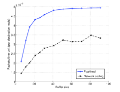
(a) Throughputs ($\lambda=0.005,N=100$)

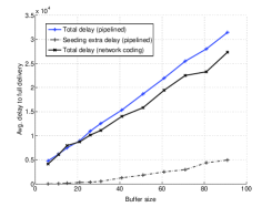
(b) Delays ($\lambda=0.005,N=100$)

Figure 2: Performance evaluation of the pipelining protocol (averaged over 100 source-generated packet batches)

Our conclusions would seem to contradict the results of Ahlswede et al.[12] and Deb et al.[3]; this is however not the case, because we complement in fact the two papers for the case of intermittently connected networks. Firstly, RLNC would reach the maxflow-mincut bound when $\nu\rightarrow+\infty$, which would mean very large buffers (not possible in our case). Secondly, [3] assumes equal initial packet spread, assumption which does not hold in DTNs with usual forwarding protocols.

VI Conclusions

In this paper we consider the problem of optimizing throughput in intermittently connected networks, with minimal impact on delay. We specifically address the practical case of limited buffers. It is proven that network coding underutilizes the available resources. Following information theoretical hints, we design a practical forwarding protocol relying on pipelining, which achieves asymptotically reliable delivery and outperforms network coding in throughput, energy consumption and memory usage with negligible delay overhead. DTNs are shown to be very sensitive to initial forwarding conditions (in particular, initial number of packet copies). Setting them to convenient values is easily achieved and yields significant performance gains. On the other hand, trying to control the network after the initiation of the forwarding process is much more challenging. Our analysis of the single source broadcast generalizes to uni- and multicast. A thorough consideration of energy constraints, congestion, multiple unsynchronized sources, comparison with other coding techniques, improved pipelining and applicability of the maximum-entropy principle to other mobility models is left for future work.

Appendix

VI-A Remarks Regarding the Equivalence Between $\Delta$ and $\Gamma$

To see why the equivalence holds, we can consider the effect of the initial packet density distribution on both schemes. Let us assume that out of the $\nu$ coded packets, the source has managed to send to the network only $\psi<\nu$. These packets have the normalized density distributions $\rho^{\prime}_{1},\rho^{\prime}_{2},\rho^{\prime}_{3},\ldots,\rho^{\prime}_{\psi}$, meaning that $\rho^{\prime}_{j}=0,(\forall)j=\overline{\psi+1,\nu}$. Clearly, due to the uniformity of the mobility model, the probability distribution for having already received these packets is the same across nodes. Let us assume w.l.o.g. that no coded packets from the source have been yet coded together. The higher the entropy, the higher is the chance that the distribution is very skewed. This means that some packets have already achieved high spread, while most others have only a few copies in the network. Then, the chance that two nodes in the next contact have exactly the same buffer content is very high. In this case, both $\Gamma$ and $\Delta$ generate the same inefficient contacts. Even if their buffers are not exactly the same, the overlap will be anyway significant. The contact will deliver with a high probability an independent packet to destination, but the problem is that most contacts in the network generate new random vectors from the same very few linear subspaces of similar dimension. For this reason, a node having received a network coded packet is still very likely to deliver during its next contact a vector which is already in the linear subspace of the receiving node. The essential observation to be made is that $\Gamma$ does not promote packets of lower densities better than $\Delta$. A rare packet will be coded together with others at basically the same rate as the one at which $\Delta$ promotes it. Indeed, the nodes receiving a rare packet will be able to deliver new combinations to others (under $\Gamma$), since the combinations contain the new packet. But this happens exactly the same under $\Delta$ too, anyway. As the buffers will be almost identical, the nodes having the rare packets will have to send them anyway, just like in $\Gamma$, because almost all the others that they have are already present in the nodes they meet. In other words, nodes receive new degrees of freedom at the same rate, both under $\Delta$ and $\Gamma$. What matters, is that a new independent vector has been received, but also the way it was obtained. If most nodes receive independent vectors generated from the same few bases, then in the next step they will for sure deliver redundant packets. As the source disseminates the initial base $\{p_{1},p_{2},p_{3},\ldots,p_{\nu}\}$ in the network during its contacts, it matters which packets of the initial base have reached destination nodes, and not the way these packets have been combined by the network. The assumption we made above that we first regard a network which has not coded yet packets together is indeed without loss of generality precisely for this reason. These simple facts provide us with the result that the behavior of both $\Delta$ and $\Gamma$ is almost identical. $\Delta$ can therefore be used as a very good approximation for $\Gamma$, where this is necessary for tractability reasons.

VI-B Impact of Entropy on Contact Efficiency

Fig. 3(a)-3(c) show contact efficiency for the same three mobility traces used in Fig. 1(a)-1(b). It can be clearly seen that high entropies allow the number of efficient contacts per unit of time to increase very fast and to remain at high levels, therefore improving throughputs, as opposed to the low entropy case. Low entropy will always generate much less efficient contacts, with negative effects as both ways of the bidirectional links established during contacts are affected.

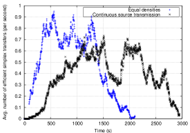
(a) Random mobility with seed no. 1

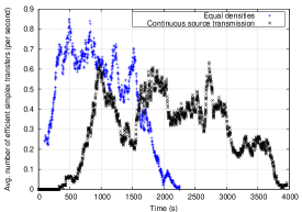
(b) Random mobility with seed no. 2

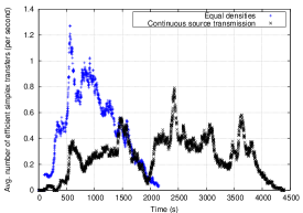
(c) Random mobility with seed no. 3

Figure 3: Average number of efficient contacts per unit of time (over a sliding window of 50 contacts), for protocols 1. (black) and 3. (blue).

References

- [1] A. Vahdat and D. Becker, “Epidemic routing for partially-connected ad hoc networks,” Duke University, Tech. Rep. CS-2000-06, 2000.
- [2] R. Subramanian and F. Fekri, “Throughput performance of network-coded multicast in an intermittently-connected network,” in Modeling and Optimization in Mobile, Ad Hoc and Wireless Networks (WiOpt), 2010 Proceedings of the 8th International Symposium on, 31 2010.
- [3] S. Deb, M. Médard, and C. Choute, “Algebraic gossip: a network coding approach to optimal multiple rumor mongering,” IEEE/ACM Trans. Netw., vol. 14, pp. 2486–2507, June 2006. [Online]. Available: http://dx.doi.org/10.1109/TIT.2006.874532
- [4] J. Widmer and J.-Y. Le Boudec, “Network coding for efficient communication in extreme networks,” in Proceedings of the 2005 ACM SIGCOMM workshop on Delay-tolerant networking, ser. WDTN ’05. New York, NY, USA: ACM, 2005, pp. 284–291. [Online]. Available: http://doi.acm.org/10.1145/1080139.1080147
- [5] Y. Lin, B. Liang, and B. Li, “Performance modeling of network coding in epidemic routing,” in Proceedings of the 1st international MobiSys workshop on Mobile opportunistic networking, ser. MobiOpp ’07. New York, NY, USA: ACM, 2007, pp. 67–74. [Online]. Available: http://doi.acm.org/10.1145/1247694.1247709
- [6] Y. Lin, B. Li, and B. Liang, “Efficient network coded data transmissions in disruption tolerant networks,” in INFOCOM 2008. The 27th Conference on Computer Communications. IEEE, 2008, pp. 1508 –1516.
- [7] E. Altman, F. De Pellegrini, and L. Sassatelli, “Dynamic control of coding in delay tolerant networks,” in INFOCOM, 2010 Proceedings IEEE, 2010, pp. 1 –5.
- [8] R. Groenevelt, P. Nain, and G. Koole, “Message delay in manet,” in Proceedings of the 2005 ACM SIGMETRICS international conference on Measurement and modeling of computer systems, ser. SIGMETRICS ’05. New York, NY, USA: ACM, 2005, pp. 412–413. [Online]. Available: http://doi.acm.org/10.1145/1064212.1064280
- [9] T. Ho, M. Médard, J. Shi, M. Effros, and D. R. Karger, “On randomized network coding,” in Proc. Allerton, Oct. 2003.
- [10] P. A. Chou, Y. Wu, and K. Jain, “Practical network coding,” in Proc. Allerton, Oct. 2003.
- [11] T. Spyropoulos, T. Turletti, and K. Obraczka, “Routing in delay-tolerant networks comprising heterogeneous node populations,” Mobile Computing, IEEE Transactions on, vol. 8, no. 8, pp. 1132 –1147, 2009.
- [12] R. Ahlswede, N. Cai, S.-Y. Li, and R. Yeung, “Network information flow,” Information Theory, IEEE Transactions on, vol. 46, no. 4, pp. 1204 –1216, Jul. 2000.