DESY 11–032

DO–TH 11/06

SFB-CPP/11–19

LPN 11–19

April 2011

$O(\alpha_{s})$ Heavy Flavor Corrections to

Charged Current Deep-Inelastic Scattering

in Mellin Space

J. Blümlein, A. Hasselhuhn, P. Kovacikova, S. Moch

Deutsches Elektronen–Synchrotron, DESY,
Platanenallee 6, D–15738 Zeuthen, Germany

We provide a fast and precise Mellin-space implementation of the $O(\alpha_{s})$ heavy flavor Wilson coefficients for charged current deep inelastic scattering processes. They are of importance for the extraction of the strange quark distribution in neutrino-nucleon scattering and the QCD analyses of the HERA charged current data. Errors in the literature are corrected. We also discuss a series of more general parton parameterizations in Mellin space.

1 Introduction

The scale evolution in Quantum Chromodynamics (QCD) can be performed very efficiently in Mellin space. There the evolution equations of the twist–2 parton distributions and the corresponding observables become ordinary differential equations, unlike in momentum-fraction space, where integro-differential equations have to be solved numerically. In Mellin space, moreover, the evolution equations can be solved analytically, provided that the anomalous dimensions and Wilson coefficients can be represented at complex values of the Mellin variable $N$, cf. [1]. The transformation mediating between both representations is

$$\mbox{\rm\bf M}\left[f(x)\right](N)=\int_{0}^{1}dx~{}x^{N-1}~{}f(x)~{},$$ (1)

where $f(x)$ may be distribution valued. The anomalous dimensions and massless Wilson coefficients to 3–loop order are functions of the nested harmonic sums [2, 3], see Refs. [4]. The nested harmonic sums $S_{\vec{a}}(N)$ are meromorphic functions in the complex plane with poles at the non positive integers and in case that the first $k$ indices $a_{i}$ are equal to one, they diverge $\propto\ln^{k}(N)$ for large values of $N$, [5]. They obey recursion relations for arguments $N\rightarrow(N+1)$ in terms of harmonic sums of lower weight, which allow for shifts parallel to the real axis. Moreover, analytic asymptotic representations have been derived, [5, 6], which are valid in the region of large values of $N,|\text{arg}(N)|<\pi$. One may derive effective numerical representations using the MINIMAX-method [7], cf. [8, 9]. In this way the QCD observables at the level of twist-2 are represented analytically at general scales $Q^{2}$, parameterizing the parton density functions by appropriate non-perturbative distributions at a starting scale $Q_{0}^{2}$. This also applies for a wide class of other processes, cf. [10].

In many precision analyses heavy quark contributions have to be considered, which are more difficult to represent in Mellin space. For deep-inelastic scattering the contributions up to the $O(\alpha_{s}^{2})$ neutral current heavy flavor Wilson coefficients [11], which are available in semi-analytic form in momentum fraction space, were given in Mellin space in Ref. [12]. The running mass effects have been described in [13].

In the present note a fast and precise implementation of the $O(\alpha_{s})$ charged current heavy-flavor Wilson coefficients for deep-inelastic scattering is presented. In Section 2 we derive the corresponding Mellin-space representations for the charged current structure functions up to $O(\alpha_{s})$. As a significant part of the data emerges for large values of $Q^{2}$, we also derive the representation in Section3 which is valid for $Q^{2}\gg m_{c}^{2}$, with $Q^{2}=-q^{2}$, $q$ being the four-momentum transfer, and $m_{c}$ the charm quark mass. We illustrate the precision of the Mellin-space implementation by comparing to the structure functions in momentum fraction space in Section 4 . Finally we remark on the Mellin space implementations of various $x$-space distributions used in different analyses in the literature in Section 5, which may be important to account for a higher flexibility in the choice of the non-perturbative input distributions. This will allow to perform analogous analyses in Mellin space in the future.

2 The Scattering Cross Section

The charged current deep-inelastic scattering cross section for $\nu(\overline{\nu})p\rightarrow l(\overline{l})+X,~{}~{}~{}l(\overline{l})p\rightarrow\nu(\overline{\nu})+X$ in case of charm-quark production is given by

$$\frac{d^{2}\sigma}{dxdy} = \frac{G_{F}^{2}S}{4\pi}\frac{M_{W}^{4}}{(M_{W}^{2}+Q^{2})^{2}}\Biggl{\{}y^{2}2x\mathbb{F}_{1}^{c}(x,Q^{2},m_{c}^{2})+2\left(1-y-y^{2}\frac{M^{2}x^{2}}{Q^{2}}\right)\mathbb{F}_{2}^{c}(x,Q^{2},m_{c}^{2})$$

$$\pm\left[1-(1-y)^{2}\right]x\mathbb{F}_{3}^{c}(x,Q^{2},m_{c}^{2})\Biggr{\}}.$$ (2)

Here $x=Q^{2}/yS,y=q.P/l.P$ are the Bjorken variables, $l$ and $P$ are the lepton and nucleon momentum, $S=2l.P$, $G_{F}$ is the Fermi constant, $M_{W}$ the mass of the $W$-boson, $M$ the nucleon mass, and $\mathbb{F}_{i}(x,Q^{2})$ are the structure functions. The $\pm$ signs in (2) refer to incoming neutrinos (anti-neutrinos) or charged leptons (anti-leptons), respectively. Note that the scattering cross section does depend on the masses of the initial state particles, cf. [14]. Due to the inclusive kinematics the dependence on $m_{c}$ is only implicit.

In the twist-2 approximation, invoking the parton model, one may decompose the nucleon wave function into individual partons and consider the excitation of single charm quarks in the transitions

$${s}^{\prime}=s~{}|V_{cs}|^{2}+d~{}|V_{cd}|^{2}\rightarrow c,~{}~{}~{}~{}~{}~{}~{}~{}~{}~{}\bar{s}^{\prime}=\bar{s}~{}|V_{cs}|^{2}+\bar{d}~{}|V_{cd}|^{2}\rightarrow\bar{c}~{},$$ (3)

with $V_{ij}$ the CKM matrix elements [15], and $s$ and $d$ the strange and down quark parton distributions. Here $\bar{d}$ and $\bar{s}$ denote the corresponding anti-quark distributions. For this transition the Bjorken variable $x$ and the momentum fraction of the struck parton $\xi$ are related by

$$x=\xi\lambda\leq\lambda~{}.$$ (4)

with $\lambda={Q^{2}}/(Q^{2}+m_{c}^{2})$. This phenomenon is called slow rescaling [16]. The heavy quark structure functions and parton densities can be expressed as a function of $\xi\in[0,1]$, preserving Mellin symmetry.

The $O(\alpha_{s})$ charged current heavy-flavor Wilson coefficients were calculated in [17] and corrected in [18] later. We will follow Ref. [18] and work in the fixed flavor number scheme (FFNS).  We define

$${\mathcal{F}}_{1}^{c}=\mathbb{F}_{1}^{c},\quad{\mathcal{F}}_{2}^{c}=\mathbb{F}_{2}^{c}/2\xi,\quad{\mathcal{F}}_{3}^{c}=\mathbb{F}_{3}^{c}/2$$ (5)

To $O(\alpha_{s})$ one obtains, after a Mellin transformation (1) over $\xi$,

$${\mathcal{F}}_{i}^{c}(N,Q^{2}) = {s^{\prime}}(N,\mu^{2})+a_{s}\Biggl{[}H_{i}^{(1),q}\left(N,\frac{m^{2}}{\mu^{2}},\frac{Q^{2}}{\mu^{2}}\right){s^{\prime}}(N,\mu^{2})+H_{i}^{(1),g}\left(N,\frac{m^{2}}{\mu^{2}},\frac{Q^{2}}{\mu^{2}}\right)g(N,\mu^{2})\Biggr{]}~{},$$

for $W^{+}$ exchange. In case of $W^{-}$ exchange $\bar{s}^{\prime}$ replaces $s^{\prime}$. Here $a_{s}=\alpha_{s}/(4\pi)$ denotes the strong coupling constant and $g$ the gluon distribution. The massive Wilson coefficients for charged current deep-inelastic scattering in Mellin space are given by

$$H_{i}^{q}\left(N,\frac{m^{2}}{\mu^{2}},\frac{Q^{2}}{\mu^{2}}\right) = 1+\sum_{k=1}^{\infty}a_{s}^{k}H_{i}^{(k),q}\left(N,\frac{m^{2}}{\mu^{2}},\frac{Q^{2}}{\mu^{2}}\right)$$ (7)

$$H_{i}^{g}\left(N,\frac{m^{2}}{\mu^{2}},\frac{Q^{2}}{\mu^{2}}\right) = \sum_{k=1}^{\infty}a_{s}^{k}H_{i}^{(k),g}\left(N,\frac{m^{2}}{\mu^{2}},\frac{Q^{2}}{\mu^{2}}\right)$$ (8)

with

$$H_{i}^{(1),q}\left(N,\frac{m^{2}}{\mu^{2}},\frac{Q^{2}}{\mu^{2}}\right) = \frac{1}{2}P_{qq}^{(0)}(N)\ln\left(\frac{Q^{2}+m_{c}^{2}}{\mu^{2}}\right)+h_{i}^{q}(\lambda,N),~{}~{}i=1,2,3,$$ (9)

$$H_{1,2}^{(1),g}\left(N,\frac{m^{2}}{\mu^{2}},\frac{Q^{2}}{\mu^{2}}\right) = \frac{1}{4}P_{qg}^{(0)}(N)\ln\left(\frac{Q^{2}+m_{c}^{2}}{\mu^{2}}\right)+\frac{1}{4}\tilde{P}(\lambda,N)+h_{1,2}^{g}(\lambda,N)$$ (10)

$$H_{3}^{(1),g}\left(N,\frac{m^{2}}{\mu^{2}},\frac{Q^{2}}{\mu^{2}}\right) = \frac{1}{4}P_{qg}^{(0)}(N)\ln\left(\frac{Q^{2}+m_{c}^{2}}{\mu^{2}}\right)-\frac{1}{4}\tilde{P}(\lambda,N)+h_{3}^{g}(\lambda,N)~{}.$$ (11)

Here the leading order splitting functions are

$${P}_{qq}^{(0)}(N) = 4C_{F}~{}\left[\frac{3}{2}+\frac{1}{N(N+1)}-2S_{1}(N)\right]$$ (12)

$${P}_{qg}^{(0)}(N) = 8T_{F}~{}\frac{N^{2}+N+2}{N(N+1)(N+2)}~{},$$ (13)

with $T_{F}=1/2,C_{F}=(N_{c}^{2}-1)/(2N_{c})$ for $SU(N_{c})$ and $N_{c}=3$ for QCD. The function $\tilde{P}(\lambda,N)$ is given by

$$\tilde{P}(\lambda,N) = \mbox{\rm\bf M}\left[P_{qg}^{(0)}(z)\ln\frac{1-\lambda z}{(1-\lambda)z}\right](N)$$ (14)

$$= 8T_{F}\Biggl{\{}\frac{\left[\lambda^{2}\left(N^{2}+3N+2\right)-2\lambda\left(N^{2}+2N\right)+2N^{2}+2N\right]}{\lambda N(N+1)(N+2)}\left[F_{2}(\lambda,N)-\frac{1}{\lambda}\ln(1-\lambda)\right]$$

$$+\frac{\lambda\left(N^{2}+3N+2\right)-2N^{2}}{\lambda N^{2}(N+1)(N+2)}\Biggr{\}}~{}.$$

In the limit $\lambda\rightarrow 1$ it takes the form

$$\tilde{P}(1,N) = 8T_{F}\left\{\frac{N^{2}+N+2}{N(N+1)(N+2)}\left[\ln\left(\frac{Q^{2}}{m^{2}}\right)-S_{1}(N)\right]+\frac{-N^{2}+3N+2}{N^{2}(N+1)(N+2)}\right\}~{}.$$ (15)

The functions ${h}_{i}^{q(g)}(\lambda,N)$ read :

$${h}_{1}^{q}(\lambda,N) = C_{F}\Biggl{[}4F_{1}(\lambda,N)-\frac{\left[\lambda^{2}\left(N^{3}+N+2\right)-\lambda\left(N^{3}+3N^{2}+4N\right)+2N^{2}+2N\right]}{\lambda N(N+1)}F_{2}(\lambda,N)$$ (16)

$$+\frac{4\left(N^{2}+N-1\right)}{N(N+1)}S_{1}(N)+4S_{1}^{2}(N)-\frac{(1-\lambda)\left[\lambda\left(N^{2}+3N+4\right)-2N-2\right]}{\lambda^{2}(N+1)}\ln(1-\lambda)$$

$$-\frac{\left[\lambda(9N^{3}+8N^{2}-5N-2)-2N^{2}\right]}{\lambda N^{2}(N+1)}\Biggr{]}$$

$${h}_{2}^{q}(\lambda,N) = C_{F}\Biggl{[}4F_{1}(\lambda,N)+\frac{\left[4\lambda^{2}\left(N^{2}+N\right)-\lambda\left(N^{3}+2N^{2}+3N+2\right)+N^{3}-N^{2}\right]}{N(N+1)}F_{2}(\lambda,N)$$ (17)

$$+\frac{4\left(N^{2}+N-1\right)}{N(N+1)}S_{1}(N)+4S_{1}^{2}(N)+\frac{(1-\lambda)\left[4\lambda(N+1)-N^{2}+N\right]}{\lambda(N+1)}\ln(1-\lambda)$$

$$+\frac{\left[4\lambda(N^{2}+N)-9N^{3}-6N^{2}+N+2\right]}{N^{2}(N+1)}\Biggr{]}$$

$${h}_{3}^{q}(\lambda,N) = C_{F}\Biggl{[}4F_{1}(\lambda,N)-\frac{(N-1)\left[\lambda(N^{2}-N-2)-N^{2}\right]}{N(N+1)}F_{2}(\lambda,N)+\frac{4\left(N^{2}+N-1\right)}{N(N+1)}S_{1}(N)$$ (18)

$$+4S_{1}^{2}(N)-\frac{(1-\lambda)\left(N^{2}+N+2\right)}{\lambda(N+1)}\ln(1-\lambda)-\frac{(3N+2)\left(3N^{2}-1\right)}{N^{2}(N+1)}\Biggr{]}$$

$${h}_{1}^{g}(\lambda,N) = -4T_{F}\Biggl{[}\frac{\left[\lambda^{2}(2N^{3}+3N^{2}+7N+2)-\lambda(2N^{3}+4N^{2}+8N)+2N^{2}+2N\right]}{2\lambda N(N+1)(N+2)}F_{2}(\lambda,N)$$ (19)

$$+\frac{\left(N^{2}+N+2\right)}{N(N+1)(N+2)}S_{1}(N)+\frac{(1-\lambda)\left[\lambda(N^{2}+N+3)-N-1\right]}{\lambda^{2}(N+1)(N+2)}\ln(1-\lambda)$$

$$+\frac{\lambda(2N^{3}+N^{2}+N-2)-2N^{2}}{2\lambda N^{2}(N+1)(N+2)}\Biggr{]}$$

$${h}_{2}^{g}(\lambda,N) = -4T_{F}\Biggl{\{}\Biggl{[}\frac{\left[\lambda^{3}(2N^{3}-6N^{2}+4N)+\lambda^{2}(-2N^{3}+7N^{2}-N+2)-\lambda(2N^{2}+4N)\right]}{2\lambda N(N+1)(N+2)}$$

$$+\frac{1}{\lambda(N+2)}\Biggr{]}F_{2}(\lambda,N)+\frac{(1-\lambda)\left[\lambda^{2}(N^{2}-3N+2)+\lambda-N-1\right]}{\lambda^{2}(N+1)(N+2)}\ln(1-\lambda)$$

$$+\frac{\left(N^{2}+N+2\right)}{N(N+1)(N+2)}S_{1}(N)+\frac{\lambda^{2}(2N^{3}-6N^{2}+4N)-\lambda(N^{2}+3N)-2\lambda-2N^{2}}{2\lambda N^{2}(N+1)(N+2)}\Biggr{\}}$$

$${h}_{3}^{g}(\lambda,N) = -4T_{F}\Biggl{[}\frac{\left(\lambda^{2}(N^{2}-N+2)+\lambda(2N^{2}+4N)-2N^{2}-2N\right)}{2\lambda N(N+1)(N+2)}F_{2}(\lambda,N)$$

$$+\frac{\left(N^{2}+N+2\right)}{N(N+1)(N+2)}S_{1}(N)-\ln(1-\lambda)\frac{(1-\lambda)(\lambda-N-1)}{\lambda^{2}(N+1)(N+2)}$$

$$-\frac{\lambda(N^{2}+3N+2)-2N^{2}}{2\lambda N^{2}(N+1)(N+2)}\Biggr{]}~{}.$$ (21)

Here $S_{k}(N)$ are the single harmonic sums [2, 3]

$$S_{k}(N)=\frac{(-1)^{k+1}}{(k-1)!}\psi^{(k-1)}(N+1)+\zeta_{k},k\in\mathbb{N}\backslash\{0\}$$ (22)

and $F_{1,2}(\lambda,N)$ denote the functions

$$F_{1}(\lambda,N) = \int_{0}^{1}dx\;\frac{x^{N}-1}{x-1}\ln(1-\lambda x)$$ (23)

$$F_{2}(\lambda,N) = \int_{0}^{1}dx\;\frac{x^{N}-1}{1-\lambda x}~{}.$$ (24)

We refer to $H_{2}^{(1),g}$ for $Q^{2}=\mu^{2}$ also in the form

$$H_{2}^{(1),g}(\lambda,N) = 4T_{F}\Biggl{\{}\frac{4-2N(N-3)-N(N^{2}+N+2)\{2S_{1}(N)+\ln[\lambda(1-\lambda)]\}}{2N^{2}(N+1)(N+2)}$$

$$+\frac{8-18(1-\lambda)+12(1-\lambda)^{2}}{(N+1)(N+2)}+\frac{(1-\lambda)_{2}F_{1}(1,N,N+1;\lambda)}{N}-\frac{1}{N}$$

$$+6\lambda(1-\lambda)\Biggl{[}\frac{{}_{2}F_{1}(1,N+1,N+2;\lambda)}{(N+1)^{2}}-2\frac{{}_{2}F_{1}(1,N+1,N+2;\lambda)-1}{(N+1)(N+2)}\Biggr{]}\Biggr{\}}$$

to correct Eq. (70) in Ref. [20]. Here, ${}_{2}F_{1}$ denotes the Gauß’ hypergeometric function

$${}_{2}F_{1}(\eta,N+\alpha+1,N+\alpha+\beta+2;\xi)=\frac{1}{B(N+\alpha+1,\beta+1)}\int_{0}^{1}~{}dzz^{N+\alpha}(1-z)^{\beta}(1-\xi z)^{-\eta}.$$

$k\backslash\lambda$	$0.1$	$0.5$	$0.9$
0	+9.999999999999999999	+1.999999999999954543	+1.111110872017648708
1	+0.821423460E-22	+0.1975123084486687E-10	+0.000098847800695649
2	$-$0.050000000000000000	$-0.250000001423445310$	$-0.456776649795426910$
3	$-0.001666666666666666$	$-0.041666626227537189$	+0.048001787041481484
4	$-0.000083333333333336$	$-0.010417267014473893$	$-2.639926313632337045$
5	$-$0.499999999997477753E-05	$-$0.003119649969153064	+21.74650303005800508
6	$-$0.333333333484935779E-06	$-$0.001072643292472726	$-$119.2024353694977123
7	$-$0.238095231857886535E-07	$-$0.000249816388951957	+442.8630812379568060
8	$-$0.178571609458723466E-08	$-$0.000477192766818736	$-$1147.492168730891145
9	$-$0.138885135219891312E-09	+0.000607438245655042	+2095.900562359927839
10	$-$0.111166985797600287E-10	$-$0.000939620170907808	$-$2688.830619105423874
11	$-$0.903191209860331475E-12	+0.000876266420390668	+2371.811788035594662
12	$-$0.800460593905461726E-13	$-$0.000571683728308967	$-$1370.383159208738358
13	$-$0.439528295242656941E-14	+0.000219008887781703	+467.1985539745224063
14	$-$0.107994848505839019E-14	$-$0.000041032031472769	$-$71.30766062862566906

Table 1: The expansion coefficients $a_{k}$, Eq. (33) for special values of $\lambda$.

Many of the contributing functions have known Mellin transforms given before in [2, 3]. Their analytic continuations to complex values of $N$ are known, cf. [5, 6, 8, 9]. The new functions (23,24) are solely related to integrals of the kind (2) for $N\in\mathbb{N}$. They obey the following recursion relations

$$F_{1}(\lambda,N+1) = F_{1}(\lambda,N)+\frac{\lambda}{N+1}F_{2}(\lambda,N+1)$$ (27)

$$F_{2}(\lambda,N+1) = \frac{1}{\lambda}\left[F_{2}(\lambda,N)-\frac{1}{N+1}-\frac{1-\lambda}{\lambda}\ln(1-\lambda)\right]~{}.$$ (28)

The singularity structure of $F_{1,2}(\lambda,N)$ for $N\in\mathbb{C}$ can be seen using the representation

$$F_{1}(\lambda,N) = -\sum_{l=1}^{\infty}\frac{\lambda^{l}}{l}\left[\psi(l+N+1)-\psi(l+1)\right]$$ (29)

$$F_{2}(\lambda,N) = -N\sum_{l=0}^{\infty}\frac{\lambda^{l}}{(N+l+1)(l+1)}~{},$$ (30)

where $\psi^{(k)}(z),k\geq 0$ denotes the polygamma function. Both functions possess poles in $N$ at negative integers.

For $F_{1}(\lambda,N)$ one may derive a sufficiently precise representation using the MINIMAX-method. The function $F_{1}$ can be written as

$$F_{1}(\lambda,N) = -\left\{\frac{1}{\lambda}-N\mathcal{E}(\lambda,1)+\sum_{l=0}^{14}a_{l}~{}\left\{N-1-l[S_{1}(N+l-1)-S_{1}(l)]\right\}\right\}~{},$$ (31)

$$\mathcal{E}(\lambda,x) \equiv \frac{1}{\lambda}(1-\lambda x)(1-\ln(1-\lambda x))~{}.$$ (32)

The function $\mathcal{E}$ under the integral is approximated by the adaptive polynomial, cf. Table 1,

$$\mathcal{E}(\lambda,x)=\sum_{k=0}^{14}a_{k}(\lambda)~{}x^{k}~{}.$$ (33)

Knowing the difference equations (27,28) one may shift $F_{1,2}$ parallel to the real axis. Usually one attempts to shift towards the asymptotic region and applies an analytic representation there. However, as sometimes recommended, one may also turn the view [21], and rather consider $F_{1,2}(\lambda,N)$ inside the unit circle, to obtain an even more beautiful result :

$$F_{1}(\lambda,N) = -\frac{1}{2}\left[S_{1}^{2}(N)+S_{2}(N)\right]$$ (34)

$$-\sum_{k=1}^{\infty}(-N)^{k}\left\{\mbox{Li}_{k+2}(\lambda)-\zeta_{k+2}+H_{1,k+1}(\lambda)-H_{1,k+1}(1)\right\}$$

$$F_{2}(\lambda,N) = \frac{1}{\lambda}\left\{\sum_{k=1}^{\infty}(-N)^{k}\left[\mbox{Li}_{k+1}(\lambda)-1\right]-\frac{N}{N+1}\right\},$$ (35)

for $|N|<1$. Here, $\mbox{Li}_{k}(x)$ denotes the classical polylogarithm [22], $H_{\vec{a}}(x)$ a harmonic polylogarithm [23],

$$H_{1,k}(x):=\int_{0}^{x}~{}dz~{}\frac{\mbox{Li}_{k}(z)-\zeta_{k}}{1-z}~{},$$ (36)

and $\zeta_{k}$ Riemann’s $\zeta$-function at an integer argument. In the limit $\lambda\rightarrow 1$ one obtains

$$F_{1}(1,N) = -\frac{1}{2}\left[S_{1}^{2}(N)+S_{2}(N)\right]$$ (37)

$$F_{2}(1,N) = -S_{1}(N)~{}.$$ (38)

The serial representations (34, 35) are quickly converging and deliver even more precise results than using (31, 33). The contour integral is performed along the line $(-\infty,-a),(c,-a),(c,a),(-\infty,a)$, with $a=0.5$. The choice of the parameter $c$ depends also on the rightmost singularity of the non-perturbative distribution $f(x)$ and was chosen with $c=1.5$ in the figures given below. The inverse Mellin transform is obtained by

$$f(x)=\frac{1}{\pi}\left\{-\int_{-\infty}^{c}{\sf Im}\left[x^{-s-ia}\mbox{\rm\bf M}[f](s+ia)\right]ds+\int_{0}^{a}{\sf Im}\left[ix^{-is-c}\mbox{\rm\bf M}[f](is+c)\right]ds\right\}~{}.$$ (39)

We extended the integral to 1000 units parallel to the real axis. The recursion relations (27, 28) together with the series (34, 35) allow to compute $F_{1,2}(\lambda,N)$ along the integration contour. Here usually the first 30 terms in the infinite sums (34, 35) provide sufficient accuracy.

3 The Massive Wilson Coefficients in the Asymptotic Region

In many applications the value of $\lambda$ becomes close to one. Within this kinematic region $Q^{2}\gg m_{c}^{2}$ the Wilson coefficients take a simpler form, and the functions needed to express them are only harmonic sums. This has been shown up to 3-loop order in case of neutral current deep-inelastic scattering in [24]. At $O(\alpha_{s})$ one obtains the following relations :

$$H_{i}^{q,(1)}\left(N,\frac{Q^{2}}{m^{2}},\frac{m^{2}}{\mu^{2}}\right) = C_{i,q}^{(1)}\left(N,\frac{Q^{2}}{\mu^{2}}\right)~{},~{}~{}~{}i=1,2,3$$ (40)

$$H_{i}^{g,(1)}\left(N,\frac{Q^{2}}{m^{2}},\frac{m^{2}}{\mu^{2}}\right) = \frac{1}{2}A_{Qg}^{(1)}\left(N,\frac{m^{2}}{\mu^{2}}\right)+C_{i,g}^{(1)}\left(N,\frac{Q^{2}}{\mu^{2}}\right)~{},~{}~{}~{}i=1,2$$ (41)

$$H_{3}^{g,(1)}\left(N,\frac{Q^{2}}{m^{2}},\frac{m^{2}}{\mu^{2}}\right) = -\frac{1}{2}A_{Qg}^{(1)}\left(N,\frac{m^{2}}{\mu^{2}}\right)~{}.$$ (42)

Here, $A_{lm}^{(1)}$ denote the 1–loop massive operator matrix elements derived in the neutral current case and $C_{i,q(g)}^{(1)}$ are the massless 1-loop Wilson coefficients, [25]. Eqs. (40, 41) are derived by expanding (16–2) for $\lambda\rightarrow 1$. At $O(\alpha_{s})$ there is no pure-singlet contribution. It turns out, that $A_{qq}^{NS,(1)}$ vanishes as expected, because closed massive fermion loop contributions can occur at $O(\alpha_{s}^{2})$ earliest. In the charged current case the interaction transmutes the massless $s^{\prime}$-quark into the massive $c$-quark. The massless quark-loop contributions to $A_{Qg}^{(1)}$, occurs with a combinatorial factor $1/2$ compared to the neutral current case. These terms vanish, because the corresponding diagrams are scaleless. Because of this no quarkonic operator matrix element contributes to (40). Eqs. (40, 41) agree with Ref. [26].

The massless Wilson coefficients obey

$$C_{i,j}\left(N,\frac{Q^{2}}{\mu^{2}}\right)=\delta_{jq}+\sum_{k=1}^{\infty}a_{s}^{k}C_{i,j}^{(k)}\left(N,\frac{Q^{2}}{\mu^{2}}\right),$$ (43)

where

$$C_{i,q}^{(1)}\left(N,\frac{Q^{2}}{\mu^{2}}\right) = \frac{1}{2}P_{qq}^{(0)}(N)\ln\left(\frac{Q^{2}}{\mu^{2}}\right)+c_{i,q}^{(1)}(N)$$ (44)

$$C_{i,g}^{(1)}\left(N,\frac{Q^{2}}{\mu^{2}}\right) = \frac{1}{2}P_{qg}^{(0)}(N)\ln\left(\frac{Q^{2}}{\mu^{2}}\right)+c_{i,g}^{(1)}(N)$$ (45)

Figure 1: Relative accuracy of the charged current structure functions $\mathbb{F}_{i}$ to $O(\alpha_{s})$ at $Q^{2}=10,100,500~{}$GeV², comparing the implementation in Mellin- and $z$-space. Here both for $F_{1,2}(\lambda,N)$ the analytic representation (34, 35) and their recurrences were used.

and [33]

$${c}_{1,q}^{(1)}(N) = {c}_{2,q}^{(1)}(N)-4C_{F}\frac{1}{N+1}$$ (46)

$${c}_{2,q}^{(1)}(N) = C_{F}\Biggl{[}\frac{\left(3N^{2}+3N-2\right)}{N(N+1)}S_{1}(N)+2S_{1}^{2}(N)-2S_{2}(N)-\frac{\left(9N^{3}+2N^{2}-5N-2\right)}{N^{2}(N+1)}\Biggr{]}$$

$${c}_{3,q}^{(1)}(N) = {c}_{2,q}^{(1)}(N)-C_{F}\frac{2(2N+1)}{N(N+1)}$$ (48)

$${c}_{1,g}^{(1)}(N) = {c}_{2,g}^{(1)}(N)-T_{F}\frac{16}{(N+1)(N+2)}$$ (49)

$${c}_{2,g}^{(1)}(N) = T_{F}\Biggl{[}-\frac{4\left(N^{2}+N+2\right)}{N(N+1)(N+2)}S_{1}(N)-\frac{4(N^{3}-4N^{2}-N-2)}{N^{2}(N+1)(N+2)}\Biggr{]}$$ (50)

$${c}_{3,g}^{(1)}(N) = 0~{}.$$ (51)

We note that the global sign for Eq. (A1.17) of [26] has to be reversed. The gluonic contribution in charged current heavy quark production has been calculated before using two finite quark masses for $e^{-}p$ scattering in Refs. [27, 28, 29] and both for $e^{-}N$ and $e^{+}N$ scattering in [29]. For calculations in case of neutrino-nucleon scattering see [30]. We repeated the calculation of the gluonic contribution for a massless $s$-quark in the $\overline{\rm MS}$-scheme.

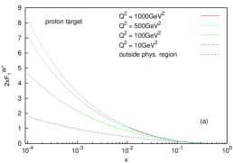
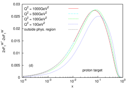
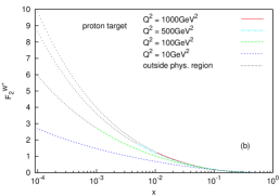
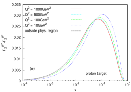
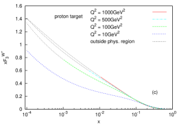
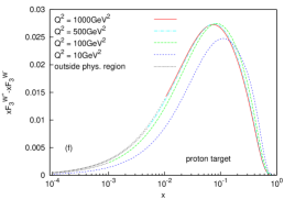
Figure 2: The charged current structure functions for charm production for different values of $Q^{2}$, using the ABKM09 parton parameterizations [31]. We indicated the kinematic range being accessible at HERA. (a)–(c) : the structure functions for $W^{+}$ exchange. (d)–(f) difference between the structure functions for $W^{+}$ and $W^{-}$ exchange.

4 Numerical Results

We compare the Mellin space representation given in Section 2 with the representation in $x$-space of Ref. [18] using the reference distribution

$$xf(x)=x^{-0.1}(1-x)^{5}$$ (52)

for both the quark and gluon densities and determine the relative accuracies $|\delta\mathbb{F}_{i}|/\mathbb{F}_{i}$ for different values of $Q^{2}$ in the massive Wilson coefficients choosing $m_{c}=1.5$ GeV and the corresponding values of $\alpha_{s}^{\rm NLO}(Q^{2})$ [31].

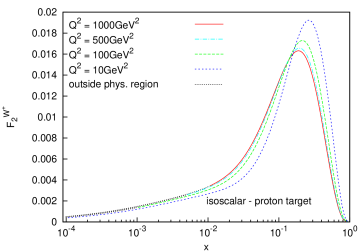
Figure 3: The difference of the structure function $\mathbb{F}_{2}$ for $W^{+}$ exchange for an isoscalar and a proton target using the ABKM09 parton distribution functions [31] in depending of $x$ and $Q^{2}$.

If one employs the MINIMAX representation relative accuracies of better than $3\times 10^{-6}$ are reached below $x=0.5$. For $x>0.5$ the relative accuracy becomes worse. In this region, however, the charm contribution is very much suppressed, as shown in Figures 2 and 3. Using the representations (34, 35) the relative accuracy is improved and amounts to $5\times 10^{-8}$ at $x=10^{-4}$ or better growing to $\sim 10^{-6}$ for $x\sim 0.4$, cf. Figure 1,a–c. Beyond this value the relative accuracy becomes worse, but also the sea quark distributions are very small in this region. For comparison we note that in [20] accuracies of 0.015 to 0.002 were obtained.

In Figure 2 we show the charged current heavy flavor structure functions $2x\mathbb{F}_{1},\mathbb{F}_{1}$ and $x\mathbb{F}_{3}$ for $ep$-scattering and the kinematics at HERA for $W^{+}$ exchange and the difference of the structure functions for $W^{+}$ and $W^{-}$ scattering using $m_{c}=1.5$ GeV, referring to the ABKM09 NLO distributions in the fixed flavor scheme [31]. Results are shown for $Q^{2}=10,100,500$ and $1000$ GeV², ($\alpha_{s}^{\rm NLO}=0.2399,0.1666,0.1379,0.1283$). The dominant contributions are those due to $W^{\pm}$–gluon fusion, which is the same for $W^{+}$ and $W^{-}$ exchange. All structure functions rise towards small values of $x$. The difference between the $W^{+}$ and $W^{-}$-exchange structure functions, on the other hand, receives its main contributions in the valence region with smaller scaling violations as in case of $W^{\pm}$–gluon fusion.

In Figure 3 the difference of the structure function $F_{2}^{W^{+}}$ for an isoscalar and proton target is shown. This also is a valence-like function. With the present precise Mellin-space implementations at hand one may perform QCD fits including the charged current heavy flavor contributions in an efficient way.

5 Parameterizations in Mellin Space

Parameterization of the non-perturbative input distribution of the parton distribution functions at a starting scale $\mu^{2}_{0}$ containing sufficient flexibility is an important condition for the QCD analyses of deep-inelastic and hard scattering data. In the literature different parameterizations of distributions are used. A wide-spread shape has the form

$$f_{i}(x,\mu_{0}^{2})=Ax^{\alpha}(1-x)^{\beta}P(x),~{}~{}P(x)=\sum_{k=1}^{K}\gamma_{k}x^{\delta_{k}}~{}.$$ (53)

The corresponding Mellin transform reads

$$f_{i}(N,\mu_{0}^{2})=A\sum_{k=1}^{K}\gamma_{k}B(N+\alpha+\delta_{k},\beta+1)~{},$$ (54)

with parameters such that $N+\alpha+\delta_{k},\beta+1\neq-l,~{}~{}\forall l\in\mathbb{N}$ and $B(x,y)=\Gamma(x)\Gamma(y)/\Gamma(x+y)$. Eq. (54) is analytic under this condition.

One may adopt the attitude to represent the non-perturbative momentum distributions of the partons, which are $L^{2}[0,1]$ measurable functions, in terms of orthogonal polynomials, see [32, 33]. If the argument of these polynomials is $x$ or a real power of $x$ one may refer to structures as (54), provided the Mellin transforms exist. The fastest convergence is obtained choosing Laguerre polynomials [34] of the argument $\ln(1/x)$, [33].

$$f_{i}(x,\mu_{0}^{2})=\sum_{k=0}^{\infty}c_{k}L_{k}\left(\ln\left(\frac{1}{x}\right)\right)~{},$$ (55)

with

$$L_{k}(z)=\sum_{l=0}^{k}\binom{k}{l}(-1)^{l}\frac{z^{l}}{l!}~{}.$$ (56)

The Mellin transform reads

$$f_{i}(N,\mu_{0}^{2})=\frac{1}{N}\sum_{k=0}^{\infty}c_{k}\left(\frac{N-1}{N}\right)^{k}~{}.$$ (57)

However, also other parameterizations are used in $x$-space analyses. One of them [35, 31] refers to the following shapes

$$f_{i}(x,\mu_{0}^{2})=Ax^{\alpha}(1-x)^{\beta}x^{ax(1+bx)},$$ (58)

partly with $b=0$. Let us first consider the simplified case $b=\beta=0$ as an illustration. Here, one obtains

$$f_{i}(N,\mu_{0}^{2})=A\sum_{k=0}^{\infty}\frac{(-a)^{k}}{(N+\alpha+k)^{k+1}}~{},$$ (59)

which is easily recognized as a quickly convergent series in $k$. In the general case we obtain

$$f_{i}(N,\mu_{0}^{2})=A\sum_{k=0}^{\infty}\frac{a^{k}}{k!}\sum_{l=0}^{k}\binom{k}{l}b^{l}\frac{\partial^{k}}{\partial N^{k}}B(N+\alpha+k+l,\beta+1).$$ (60)

The derivatives of the Beta-function in (60) can be calculated in a recursive way, see [3]. Let

$$\frac{1}{k!}\frac{\partial^{k}}{\partial N^{k}}B(N+\alpha,\beta)=B(N+\alpha,\beta)~{}\Delta_{k},~{}~{}\Delta_{0}=1~{}.$$ (61)

Then one obtains

$$\Delta_{k}=\frac{1}{k}\sum_{l=1}^{k}\Delta_{k-l}f_{l}~{},$$ (62)

with

$$f_{l}=\frac{1}{(l-1)!}\left[\psi^{(l-1)}(N+\alpha)-\psi^{(l-1)}(N+\alpha+\beta)\right]~{}.$$ (63)

Yet another parameterization was used in [36],

$$f_{i}(x,Q^{2})=Ax^{\alpha}(1-x)^{\beta}e^{\gamma x}(1+\delta x)^{\eta}.$$ (64)

We first consider the case $\delta=0$. The Mellin transform of (64) is then given by

$$f_{i}(N,Q^{2}) = A~{}B(N+\alpha,\beta+1)~{}_{1}F_{1}(\alpha+N,\beta+\alpha+N+1;\gamma)$$ (65)

$$= A~{}B(N+\alpha,\beta+1)~{}e^{\gamma}~{}_{1}F_{1}(\beta+1,N+\alpha+\beta+1;-\gamma)~{},$$

where ${}_{1}F_{1}(\alpha,\beta;z)$ denotes the confluent hypergeometric function [37]. It obeys the recursion relation [38]

$${}_{1}F_{1}(\alpha,\beta+1;z)=-\frac{1}{z(\beta-\alpha)}\left[\beta(1-\beta-z)_{1}F_{1}(\alpha,\beta;z)+\beta(\beta-1)_{1}F_{1}(\alpha,\beta-1;z)\right]~{}.$$ (66)

For large values of $N$ the asymptotic relation [38, 39]

$${}_{1}F_{1}(\beta+1,N+\alpha+\beta+1;-\gamma) = \sum_{s=0}^{n-1}\frac{\Gamma(\beta+1+s)\Gamma(N+\alpha+\beta+1)}{\Gamma(\beta+1)\Gamma(N+\alpha+\beta+s+1)}\frac{(-\gamma)^{s}}{s!}$$ (67)

$$+O\left(|N+\alpha+\beta+1|^{-n}\right)$$

holds. Eqs. (66,67) may thus be used to compute the analytic continuation of (65).

For the additional factor

$$(1+\delta x)^{\eta}$$ (68)

one may extract an integer power from $\eta$ such that the remainder,$\bar{\eta}$, obeys $\bar{\eta}\in[-1/2,1/2]$. The integer contribution $\tilde{\eta}=\eta-\bar{\eta}$ is modifying the above representations but leads to the same structure. The remaining factor possesses the well converging representation

$$(1+\delta x)^{\bar{\eta}}=\sum_{l=1}^{\infty}\binom{\bar{\eta}}{l}\delta^{l}~{}x^{l}~{},$$ (69)

and leads to a corresponding generalization of relations (65, 67).

6 Conclusions

A fast and precise Mellin-space implementation of the $O(\alpha_{s})$ massive charged current Wilson coefficients for deep-inelastic scattering is provided. This process is of relevance for the understanding of di-muon production in deep-inelastic neutrino-nucleon scattering and for the deep-inelastic charged current data measured at HERA in particular w.r.t. the extraction of the unpolarized strange-quark distribution. To represent the Wilson coefficients we used both the MINIMAX-method and completely analytic representations and exploited recurrences in the complex-valued Mellin variable $N$ for $N\rightarrow N+1$. In wide kinematic ranges relative accuracies of $10^{-7}$ and better are obtained for the deep-inelastic structure functions. Errors in the literature have been corrected. We present phenomenological applications for the structure functions $\mathbb{F}_{i}(x,Q^{2}),~{}~{}i=1,2,3$ both for $W^{+}$ and $W^{-}$ exchange. Furthermore, we provided Mellin-space representations for a wide range of representations used in different $x$-space analyses. This allows both for more flexible choices of the parton distributions at the input scale using Mellin-based codes in data analyses and for comparisons with fits given in the literature. The corresponding code is based on ANCONT [8] and available on request from Johannes.Bluemlein@desy.de.

Acknowledgment.  We would like to thank S. Alekhin for discussions and N. Temme for useful remarks. This paper has been supported in part by DFG Sonderforschungsbereich Transregio 9, Computergestützte Theoretische Teilchenphysik and EU Network LHCPHENOnet PITN-GA-2010-264564.

References

• [1] See e.g. J. Blümlein and A. Vogt, Phys. Rev.  D 58 (1998) 014020 [arXiv:hep-ph/9712546];
A. Vogt, Comput. Phys. Commun.  170 (2005) 65 [arXiv:hep-ph/0408244].
• [2] J. A. M. Vermaseren, Int. J. Mod. Phys.  A 14 (1999) 2037 [arXiv:hep-ph/9806280].
• [3] J. Blümlein and S. Kurth, Phys. Rev.  D 60 (1999) 014018 [arXiv:hep-ph/9810241].
• [4] S. Moch, J. A. M. Vermaseren and A. Vogt, Nucl. Phys.  B 688 (2004) 101 [arXiv:hep-ph/0403192];
A. Vogt, S. Moch and J. A. M. Vermaseren, Nucl. Phys.  B 691 (2004) 129 [arXiv:hep-ph/0404111];
J. A. M. Vermaseren, A. Vogt and S. Moch, Nucl. Phys.  B 724 (2005) 3 [arXiv:hep-ph/0504242]. S. Moch, J. A. M. Vermaseren and A. Vogt, Nucl. Phys.  B 813 (2009) 220 [arXiv:0812.4168 [hep-ph]].
• [5] J. Blümlein, Comput. Phys. Commun.  180 (2009) 2218 [arXiv:0901.3106 [hep-ph]].
• [6] J. Blümlein, Proceedings of the Workshop Motives, Quantum Field Theory, and Pseudodifferential Operators, held at the Clay Mathematics Institute, Boston University, June 2–13, 2008, Clay Mathematics Proceedings 12 (2010) 167–186, Eds. A. Carey, D. Ellwood, S. Paycha, S. Rosenberg, arXiv:0901.0837 [math-ph];
J. Ablinger, J. Blümlein, and C. Schneider, in preparation.
• [7] C. Lanczos, J. Math. Phys. 17 (1938) 123;
F. Lösch and F. Schoblik, Die Fakultät und verwandte Funktionen, (Teubner, Stuttgart, 1951);
C. Hastings, jr., Approximations for Digital Computers, (Princeton University Press, Princeton/NJ, 1953);
M. Abramowitz and I.A. Stegun, Handbook of Mathematical Functions, (NBS, Washington, 1964);
L.A. Lyusternik, O.A. Chervonenkis, and A.R. Yanpol’skii, Handbook for Computing of Elementary Functions, Russian ed. (Fizmatgiz, Moscow, 1963); (Pergamon Press, New York, 1964).
• [8] J. Blümlein, Comput. Phys. Commun.  133 (2000) 76 [arXiv:hep-ph/0003100].
• [9] J. Blümlein and S. O. Moch, Phys. Lett.  B 614 (2005) 53 [arXiv:hep-ph/0503188].
• [10] J. Blümlein and V. Ravindran, Nucl. Phys.  B 749 (2006) 1 [arXiv:hep-ph/0604019]; B 716 (2005) 128 [arXiv:hep-ph/0501178];
J. Blümlein and S. Klein, PoS ACAT (2007) 084 [arXiv:0706.2426 [hep-ph]];
J. Blümlein, M. Kauers, S. Klein and C. Schneider, Comput. Phys. Commun.  180 (2009) 2143 [arXiv:0902.4091 [hep-ph]].
• [11] E. Laenen, S. Riemersma, J. Smith and W. L. van Neerven, Nucl. Phys.  B 392 (1993) 162;
S. Riemersma, J. Smith and W. L. van Neerven, Phys. Lett.  B 347 (1995) 143 [arXiv:hep-ph/9411431].
• [12] S. I. Alekhin and J. Blümlein, Phys. Lett.  B 594 (2004) 299 [arXiv:hep-ph/0404034].
• [13] I. Bierenbaum, J. Blümlein and S. Klein, Nucl. Phys.  B 820 (2009) 417 [arXiv:0904.3563 [hep-ph]];
S. Alekhin and S. Moch, arXiv:1011.5790 [hep-ph].
• [14] A. Arbuzov, D. Y. Bardin, J. Blümlein, L. Kalinovskaya and T. Riemann, Comput. Phys. Commun.  94 (1996) 128 [arXiv:hep-ph/9511434];
N. Schmitz, Neutrinophysik, (Teubner, Stuttgart, 1997).
• [15] N. Cabibbo, Phys. Rev. Lett.  10 (1963) 531;
M. Kobayashi, T. Maskawa, Prog. Theor. Phys.  49 (1973) 652
• [16] E. Derman, Nucl. Phys.  B 110 (1976) 40;
R. M. Barnett, Phys. Rev. Lett.  36 (1976) 1163;
R. Barbieri, J. R. Ellis, M. K. Gaillard, G. G. Ross, Phys. Lett.  B64 (1976) 171; Nucl. Phys.  B117 (1976) 50.
• [17] T. Gottschalk, Phys. Rev.  D 23 (1981) 56.
• [18] M. Glück, S. Kretzer and E. Reya, Phys. Lett.  B 380 (1996) 171 [Erratum-ibid.  B 405 (1997) 391] [arXiv:hep-ph/9603304].
• [19] J. Blümlein and W. L. van Neerven, Phys. Lett.  B 450 (1999) 417 [arXiv:hep-ph/9811351].
• [20] R. D. Ball et al., arXiv:1101.1300v2 [hep-ph].
• [21] N. Copernicus Torinensis, De Revolutionibus orbium cœlestium, (J. Petreium, Norimbergæ, 1543).
• [22] L. Lewin, Polylogarithms and Associated Functions, (North Holland, Amsterdam, 1981).
• [23] E. Remiddi and J. A. M. Vermaseren, Int. J. Mod. Phys.  A 15 (2000) 725 [arXiv:hep-ph/9905237].
• [24] M. Buza, Y. Matiounine, J. Smith, R. Migneron and W. L. van Neerven, Nucl. Phys.  B 472 (1996) 611 [arXiv:hep-ph/9601302];
I. Bierenbaum, J. Blumlein and S. Klein, Nucl. Phys.  B 780 (2007) 40 [arXiv:hep-ph/0703285]; Phys. Lett.  B 672 (2009) 401 [arXiv:0901.0669 [hep-ph]];
I. Bierenbaum, J. Blümlein, S. Klein and C. Schneider, Nucl. Phys.  B 803 (2008) 1 [arXiv:0803.0273 [hep-ph]];
J. Blümlein, S. Klein and B. Tödtli, Phys. Rev.  D 80 (2009) 094010 [arXiv:0909.1547 [hep-ph]];
J. Ablinger, J. Blümlein, S. Klein, C. Schneider and F. Wißbrock, Nucl. Phys.  B 844 (2011) 26 [arXiv:1008.3347 [hep-ph]].
• [25] W. Furmanski and R. Petronzio, Z. Phys.  C 11 (1982) 293 and references therein.
• [26] M. Buza, W. L. van Neerven, Nucl. Phys.  B500 (1997) 301.[hep-ph/9702242].
• [27] M. Glück, R. M. Godbole, E. Reya, Z. Phys.  C38 (1988) 441; [Erratum-ibid. 39 (1988) 590].
• [28] U. Baur, J. J. van der Bij, Nucl. Phys.  B304 (1988) 451;
J. J. van der Bij, G. J. van Oldenborgh, Z. Phys.  C51 (1991) 477.
• [29] G. A. Schuler, Nucl. Phys.  B299 (1988) 21.
• [30] G. Kramer, B. Lampe, Z. Phys.  C54 (1992) 139-146.
• [31] S. Alekhin, J. Blümlein, S. Klein and S. Moch, Phys. Rev.  D 81 (2010) 014032 [arXiv:0908.2766 [hep-ph]].
• [32] F. J. Yndurain, Phys. Lett.  B74 (1978) 68. G. Parisi and N. Sourlas, Nucl. Phys.  B151 (1979) 421;
R. Kobayashi, M. Konuma, S. Kumano, Comput. Phys. Commun.  86 (1995) 264,[hep-ph/9409289]. Z. Phys.  C31 (1986) 151;
J. Chyla and J. Rames, Z. Phys.  C 31 (1986) 151.
• [33] W. Furmanski, R. Petronzio, Nucl. Phys.  B195 (1982) 237;
J. Blümlein, M. Klein, G. Ingelman and R. Rückl, Z. Phys.  C 45 (1990) 501.
• [34] E. de Laguerre, Bull. Soc. math. France 7 (1879) 72.
• [35] S. Alekhin, K. Melnikov and F. Petriello, Phys. Rev.  D 74 (2006) 054033 [arXiv:hep-ph/0606237].
• [36] J. Pumplin, D. R. Stump, J. Huston, H. L. Lai, P. M. Nadolsky and W. K. Tung, JHEP 0207 (2002) 012 [arXiv:hep-ph/0201195].
• [37] E.E. Kummer, Journal für die reine und angew. Mathematik, 17 (1837) 228.
• [38] NIST Handbook of Mathematical Functions, eds. F.W.J. Olver et al., (Cambridge University Press, Cambdrige, 2010);
N.M. Temme, Special Functions, (John Wiley & Sons, New York, 1996).
• [39] N.M. Temme, Journ. Comp. Appl. Math. 7 (1981) 27.