Spatial models generated by nested stochastic partial differential equations, with an application to global ozone mapping

Abstract

A new class of stochastic field models is constructed using nested stochastic partial differential equations (SPDEs). The model class is computationally efficient, applicable to data on general smooth manifolds, and includes both the Gaussian Matérn fields and a wide family of fields with oscillating covariance functions. Nonstationary covariance models are obtained by spatially varying the parameters in the SPDEs, and the model parameters are estimated using direct numerical optimization, which is more efficient than standard Markov Chain Monte Carlo procedures. The model class is used to estimate daily ozone maps using a large data set of spatially irregular global total column ozone data.

and

1 Introduction

Building models for spatial environmental data is a challenging problem that has received much attention over the past years. Nonstationary covariance models are often needed since the traditional stationary assumption is too restrictive for capturing the covariance structure in many problems. Also, many environmental data sets today contain massive amounts of measurements, which makes computational efficiency another increasingly important model property. One such data set, which will be analyzed in this work, is the the Total Ozone Mapping Spectrometer (TOMS) atmospheric ozone data [McPeters et al. (1996)]. The data was collected by a TOMS instrument onboard the the near-polar, Sun-synchronous orbiting satellite Nimbus-7, launched by NASA on October 24, 1978. During the sunlit portions of the satellite’s orbit, the instrument collected data in scans perpendicular to the orbital plane. A new scan was started every eight seconds as the spacecraft moved from south to north. A number of recent papers in the statistical literature [Cressie and Johannesson (2008), Jun and Stein (2008), Stein (2007)] have studied the data, and it requires nonstationary covariance structures as well as efficient computational techniques due to the large number of observations.

A covariance model that is popular in environmental statistics is the Matérn family of covariance functions [Matérn (1960)]. The Matérn covariance function has a shape parameter, $\nu$, a scale parameter, $\kappa$, and a variance parameter, $\phi^{2}$, and can be parametrized as

$$C(\mathbf{h})=\frac{2^{1-\nu}\phi^{2}}{(4\pi)^{{d/2}}\Gamma(\nu+{d/2})\kappa^{2\nu}}(\kappa\|\mathbf{h}\|)^{\nu}K_{\nu}(\kappa\|\mathbf{h}\|),\qquad\mathbf{h}\in\mathbb{R}^{d},$$ (1)

where $K_{\nu}$ is a modified Bessel function of the second kind of order $\nu>0$. One drawback with defining the model directly through a covariance function, such as (1), is that it makes nonstationary extensions difficult. Another drawback is that, unless the covariance function has compact support, the computational complexity for calculating the Kriging predictor based on $n$ measurements is $\mathcal{O}(n^{3})$. This makes the Matérn covariance model computationally infeasible for many environmental data sets.

Recently, Lindgren, Rue and Lindström (2010) derived a method for explicit, and computationally efficient, Markov representations of the Matérn covariance family. The method uses the fact that a random process on $\mathbb{R}^{d}$ with a Matérn covariance function is a solution to the stochastic partial differential equation (SPDE)

$$(\kappa^{2}-\Delta)^{{\alpha/2}}X(\mathbf{s})=\phi\mathcal{W}(\mathbf{s}),$$ (2)

where $\mathcal{W}(\mathbf{s})$ is Gaussian white noise, $\Delta$ is the Laplace operator, and $\alpha=\nu+d/2$ [Whittle (1963)]. Instead of defining Matérn fields through the covariance functions (1), Lindgren, Rue and Lindström (2010) used the solution to the SPDE (2) as a definition. This definition is valid not only on $\mathbb{R}^{d}$ but also on general smooth manifolds, such as the sphere, and facilitates nonstationary extensions by allowing the SPDE parameters $\kappa^{2}$ and $\phi$ to vary with space. The Markov representations were obtained by considering approximate stochastic weak solutions to the SPDE; see Section 3 for details.

In this paper we extend the work by Lindgren, Rue and Lindström (2010) and construct a new flexible class of spatial models by considering a generalization of (2). This model class contains a wide family of covariance functions, including both the Matérn family and oscillating covariance functions, and it maintains all desirable properties of the Markov approximated Matérn model, such as computational efficiency, easy nonstationary extensions and applicability to data on general smooth manifolds.

The model class is introduced in Section 2, with derivations of some basic properties, examples of covariance functions that can be obtained from these models and a discussion on nonstationary extensions. Section 3 gives a review of the Hilbert space approximation technique and shows how it can be extended to give computationally efficient representations also for this new model class. In Section 4 a numerical parameter estimation procedure for the nested SPDE models is presented, and the section concludes with a discussion on computational complexity for parameter estimation and Kriging prediction. In Section 5 the model class is used to analyze the TOMS ozone data. In particular, all measurements available from October 1st, 1988 in the spatially and temporally irregular “Level 2” version of the data set are used. This data set contains approximately 180,000 measurements, and the nonstationary version of the model class is used to construct estimates of the ozone field for that particular day. Finally, Section 6 contains some concluding remarks and suggestions for further work.

2 Stationary nested SPDE models

A limitation with the Matérn covariance family is that it does not contain any covariance functions with negative values, such as oscillating covariance functions. One way of constructing a larger class of stochastic fields is to consider a generalization of the SPDE (2):

$$\mathcal{L}_{1}X(\mathbf{s})=\mathcal{L}_{2}\mathcal{W}(\mathbf{s}),$$ (3)

for some linear operators $\mathcal{L}_{1}$ and $\mathcal{L}_{2}$. If $\mathcal{L}_{1}$ and $\mathcal{L}_{2}$ are commutative operators, (3) is equivalent to the following system of nested SPDEs:

$$\mathcal{L}_{1}X_{0}(\mathbf{s}) = \mathcal{W}(\mathbf{s}),$$

$$X(\mathbf{s}) = \mathcal{L}_{2}X_{0}(\mathbf{s}).$$

This representation gives us an interpretation of the consequence of the additional differential operator $\mathcal{L}_{2}$: $X(\mathbf{s})$ is simply $\mathcal{L}_{2}$ applied to the solution one would get to (3) if $\mathcal{L}_{2}$ was the identity operator. Equation (3) generates a large class of random fields, even if the operators $\mathcal{L}_{1}$ and $\mathcal{L}_{2}$ are restricted to operators closely related to (2). One of the simplest extensions of the Matérn model is to let $\mathcal{L}_{1}$ be the same as in (2) and use $\mathcal{L}_{2}=(b+\mathbf{B}^{\top}\nabla)$, where $\nabla$ is the gradient, $b\in\mathbb{R}$, and $\mathbf{B}\in\mathbb{R}^{d}$. The equation then is

$$(\kappa^{2}-\Delta)^{{\alpha/2}}X(\mathbf{s})=(b+\mathbf{B}^{\top}\nabla)\mathcal{W}(\mathbf{s}),$$ (5)

and $X(\mathbf{s})$ is a weighted sum of a Matérn field and its directional derivative in the direction determined by the vector $\mathbf{B}$. This model is closely related to the models introduced in Jun and Stein (2007) and Jun and Stein (2008), and the connection is discussed later in Section 5. To get a larger class of models, the orders of the operators $\mathcal{L}_{1}$ and $\mathcal{L}_{2}$ can be increased, and to get a class of stochastic fields that is easy to work with, the operators are written as products, where each factor in the product is equal to one of the operators in (5). Thus, let

$$\mathcal{L}_{1}=\prod_{i=1}^{n_{1}}(\kappa_{i}^{2}-\Delta)^{{\alpha_{i}/2}}$$ (6)

for $\alpha_{i}\in\mathbb{N}$ and $\kappa_{i}^{2}>0$, and use

$$\mathcal{L}_{2}=\prod_{i=1}^{n_{2}}(b_{i}+\mathbf{B}_{i}^{\top}\nabla)$$ (7)

for $b_{i}\in\mathbb{R}$ and $\mathbf{B}_{i}\in\mathbb{R}^{d}$. Hence, the SPDE generating the class of nested SPDE models is

$$\Biggl{(}\prod_{i=1}^{n_{1}}(\kappa^{2}-\Delta)^{{\alpha_{i}/2}}\Biggr{)}X(\mathbf{s})=\Biggl{(}\prod_{i=1}^{n_{2}}(b_{i}+\mathbf{B}_{i}^{\top}\nabla)\Biggr{)}\mathcal{W}(\mathbf{s}).$$ (8)

There are several alternative equations one might consider; one could, for example, let $\mathcal{L}_{2}$ be on the same form as $\mathcal{L}_{1}$, or allow for anisotropic operators on the form $(1-\nabla^{\top}\mathbf{A}\nabla)$ for some positive definite matrix $\mathbf{A}$. However, to limit our scope, we will from now on only consider model (8).

2.1 Properties in $\mathbb{R}^{d}$

In this section some basic properties of random fields generated by (8), when $\mathbf{s}\in\mathbb{R}^{d}$, are given. First note that all Matérn fields with shape parameters satisfying $\nu+d/2\in\mathbb{N}$ are contained in the class of stochastic fields generated by (8) since $(\kappa^{2}-\Delta)^{{\alpha/2}}$ can be written on the form (6) for these values of $\nu$. Also note that the order of the operator $\mathcal{L}_{2}$ cannot be larger than the order of $\mathcal{L}_{1}$ if $X(\mathbf{s})$ should be at least as “well behaved” as white noise; hence, one must have $\sum_{i=1}^{n_{1}}\alpha_{i}\geq n_{2}$. The smoothness of $X(\mathbf{s})$ is determined by the difference of the orders of the operators $\mathcal{L}_{1}$ and $\mathcal{L}_{2}$. In order to make a precise statement about this, the spectral density of $X(\mathbf{s})$ is needed.

Proposition 2.1

The spectral density for $X(\mathbf{s})$ defined by (8) is given by

$$S(\mathbf{k})=\frac{\phi^{2}}{(2\pi)^{d}}\frac{\prod_{j=1}^{n_{2}}(b_{j}^{2}+\mathbf{k}^{\top}\mathbf{B}_{j}\mathbf{B}_{j}^{\top}\mathbf{k})}{\prod_{j=1}^{n_{1}}(\kappa_{j}^{2}+\|\mathbf{k}\|^{2})^{\alpha_{j}}}.$$

This proposition is easily proved using linear filtering theory [see, for example, Yaglom (1987)]. Given the spectral density of $X(\mathbf{s})$, the following proposition regarding the sample function regularity can be proved using Theorem 3.4.3 in Adler (1981).

Proposition 2.2

$X(\mathbf{s})$ defined by (8) has almost surely continuous sample functions if $2\sum_{i=1}^{n_{1}}\alpha_{i}-2n_{2}>d$.

Because the stochastic field $X(\mathbf{s})$ is generated by the SPDE (8), the following corollary regarding sample path differentiability is also easily proved using the fact that the directional derivative of $X(\mathbf{s})$ is in the class of nested SPDE models.

Corollary 2.3

Given that $2\sum_{i=1}^{n_{1}}\alpha_{i}-2n_{2}-d>m$, the $m$th order directional derivative of $X(\mathbf{s})$, $(\mathbf{B}^{\top}\nabla)^{m}X(\mathbf{s})$, has almost surely continuous sample functions.

Hence, as $2\sum_{i=1}^{n_{1}}\alpha_{i}-2n_{2}$ increases, the sample paths become smoother, and eventually become differentiable, twice differentiable, and so on. One could also give a more precise characterization of the sample path regularity using the notion of Hölder continuity. This is (more or less) straightforward using properties of index-$\beta$ random fields [Adler (1981)], but outside the scope of this article.

A closed-form expression for the covariance function is not that interesting since none of the methods that are later presented for parameter estimation, spatial prediction or model validation require an expression for the covariance function; however, if one were to use some technique that requires the covariance function, it can be derived. An expression for the general case is quite complicated, and will not be presented here. Instead we present a recipe for calculating the covariance function for given parameters of the SPDE, with explicit results for a few examples.

To calculate the covariance function of $X(\mathbf{s})$, first calculate the covariance function, $C_{X_{0}}(\mathbf{h})$, of $X_{0}(\mathbf{s})$, given by (2). Given this covariance function, the covariance function for $X(\mathbf{s})$ is obtained as

$$C(\mathbf{h})=\Biggl{(}\prod_{i=1}^{n_{2}}(b_{i}-\nabla^{\top}\mathbf{B}_{i}\mathbf{B}_{i}^{\top}\nabla)\Biggr{)}C_{X_{0}}(\mathbf{h}).$$

The motivation for this expression is again directly from linear filter theory, and the $d$-dimensional equivalent of the formula for the covariance function for a differentiated stochastic process, $r_{X^{\prime}}(\tau)=-r_{X}^{\prime\prime}(\tau)$. To get an expression for $C_{X_{0}}(\mathbf{h})$, first use Proposition 2.1 with $\mathcal{L}_{2}=I$ to get the spectral density of $X_{0}(\mathbf{s})$. Using a partial fraction decomposition, the spectral density can be written as

$$S_{X_{0}}(\mathbf{k})=\frac{\phi^{2}}{(2\pi)^{d}}\sum_{i=1}^{n}\sum_{j=1}^{\alpha_{i}}\frac{p_{i,j}}{(\kappa_{i}^{2}+\|\mathbf{k}\|^{2})^{j}},$$ (9)

where $p_{i,j}$ is a real constant which can be found using the Heaviside cover-up method [see, for example, Thomas and Finney (1995), page 523]. Now, by taking the inverse Fourier transform of (9), the covariance function for $X_{0}(\mathbf{s})$ is

$$C_{X_{0}}(\mathbf{h})=\sum_{i=1}^{n}\sum_{j=1}^{\alpha_{i}}p_{i,j}C_{\kappa_{i}}^{j}(\mathbf{h}),$$

where $C_{\kappa}^{\nu}(\mathbf{h})$ denotes a Matérn covariance function with shape parameter $\nu$, scale parameter $\kappa$ and variance parameter $\phi^{2}$. The final step is to use that the derivative of a Matérn covariance function can be expressed using a Matérn covariance with another shape parameter. More precisely, one has

$$\frac{\partial}{\partial h_{i}}C_{\kappa}^{\nu}(\mathbf{h})=-\frac{h_{i}}{2\nu}C_{\kappa}^{\nu-1}(\mathbf{h}),$$

where $h_{i}$ denotes the $i$th component of the vector $\mathbf{h}$. Using these calculations, one can obtain the covariance function for any field given by (8). We conclude this section by showing the covariance function for some simple cases in $\mathbb{R}^{2}$. The covariance functions for these examples are shown in Figure 1, and realizations of Gaussian processes with these covariance functions are shown in Figure 2.

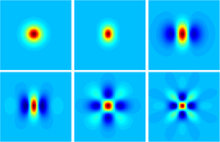
Figure 1: Covariance functions of random fields obtained from model (8) with parameters from Example 1 (top left), Example 2 (top middle and right), Example 3 (bottom left and middle) and Example 4 (bottom right).

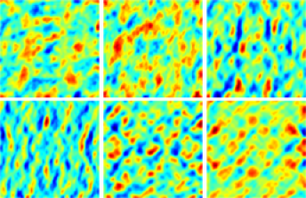
Figure 2: Realizations of random fields obtained from model (8) with different parameters. The realization in each panel corresponds to a stochastic field with the covariance function shown in the corresponding panel in Figure 1.

Example 1.

With $\mathcal{L}_{1}=(\kappa^{2}-\Delta)^{{\alpha/2}}$ and $\mathcal{L}_{2}$ as the identity operator, the standard Matérn covariance function (1) is obtained, shown in the top left panel of Figure 1.

Example 2.

The simplest nested SPDE model (5) has the covariance function

$$C(\mathbf{h})=bC_{\kappa}^{\nu}(\mathbf{h})+\frac{\mathbf{B}^{\top}\mathbf{B}}{2\nu}C_{\kappa}^{\nu-1}(\mathbf{h})-\frac{\mathbf{h}^{\top}\mathbf{B}\mathbf{B}^{\top}\mathbf{h}}{4\nu(\nu-1)}C_{\kappa}^{\nu-2}(\mathbf{h}).$$

A stochastic field with this covariance function is obtained as a weighted sum of a Matérn field $X_{0}(\mathbf{s})$ and its directional derivative in the direction of $\mathbf{B}$. The field therefore has a Matérn-like behavior in the direction perpendicular to $\mathbf{B}$ and an oscillating behavior in the direction of $\mathbf{B}$. In the upper middle panel of Figure 1, this covariance function is shown for $\mathbf{B}=(1,0)^{\top}$, $\nu=3$, and $b=5$. In the upper right panel of Figure 1, it is shown for $\mathbf{B}=(1,0)^{\top}$, $\nu=3$, and $b=0$.

Example 3.

The number of zero crossings of the covariance function in the direction of $\mathbf{B}$ is at most $n_{2}$. In the previous example we had $n_{2}=1$, and to obtain a more oscillating covariance function, the order of $\mathcal{L}_{2}$ can be increased by one:

$$(\kappa^{2}-\Delta)^{{\alpha/2}}X(\mathbf{s})=(b_{1}+\mathbf{B}_{1}^{\top}\nabla)(b_{2}+\mathbf{B}_{2}^{\top}\nabla)\mathcal{W}(\mathbf{s}).$$

This model has the covariance function

$$C(\mathbf{h}) = b_{1}b_{2}C_{\kappa}^{\nu}(\mathbf{h})+\frac{b_{2}\mathbf{B}_{1}^{\top}\mathbf{B}_{1}+b_{1}\mathbf{B}_{2}^{\top}\mathbf{B}_{2}}{2\nu}C_{\kappa}^{\nu-1}(\mathbf{h})$$

$${}+\frac{2(\mathbf{B}_{2}^{\top}\mathbf{B}_{1})^{2}+\mathbf{B}_{1}^{\top}\mathbf{B}_{1}\mathbf{B}_{2}^{\top}\mathbf{B}_{2}-\mathbf{h}^{\top}(b_{1}\mathbf{B}_{2}\mathbf{B}_{2}^{\top}+b_{2}\mathbf{B}_{1}\mathbf{B}_{1}^{\top})\mathbf{h}}{2^{2}\nu(\nu-1)}C_{\kappa}^{\nu-2}(\mathbf{h})$$

$${}-\frac{\mathbf{h}^{\top}(\mathbf{B}_{1}\mathbf{B}_{2}^{\top}\mathbf{B}_{2}\mathbf{B}_{1}^{\top}+4\mathbf{B}_{1}\mathbf{B}_{1}^{\top}\mathbf{B}_{2}\mathbf{B}_{2}^{\top}+\mathbf{B}_{2}\mathbf{B}_{1}^{\top}\mathbf{B}_{1}\mathbf{B}_{2}^{\top})\mathbf{h}}{2^{3}\nu(\nu-1)(\nu-2)}C_{\kappa}^{\nu-3}(\mathbf{h})$$

$${}+\frac{(\mathbf{B}_{1}^{\top}\mathbf{h}\mathbf{h}^{\top}\mathbf{B}_{2})^{2}}{2^{4}\nu(\nu-1)(\nu-2)(\nu-3)}C_{\kappa}^{\nu-4}(\mathbf{h}).$$

In the bottom left panel of Figure 1 this covariance function is shown for $\nu=5$, $b_{1}=b_{2}=0$ and $\mathbf{B}_{1}=\mathbf{B}_{2}=(1,0)^{\top}$. With these parameters, the covariance function is similar to the covariance function in the previous example, but with one more zero crossing in the direction of $\mathbf{B}$. For this specific choice of parameters, the expression for the covariance function can be simplified to

$$C(\mathbf{h})=3\gamma_{2}C_{\kappa}^{\nu-2}(\mathbf{h})-6\gamma_{3}h_{1}^{2}C_{\kappa}^{\nu-3}(\mathbf{h})+\gamma_{4}h_{1}^{4}C_{\kappa}^{\nu-4}(\mathbf{h}),$$

where $\gamma_{k}=(2^{k}\Pi_{i=0}^{k-1}(\nu-k))^{-1}$. In the bottom middle panel of Figure 1 the covariance function is shown for $\nu=5$, $b_{1}=b_{2}=0$, $\mathbf{B}_{1}=(1,0)^{\top}$, and $\mathbf{B}_{2}=(0,1)^{\top}$. Thus, the field $X_{0}(\mathbf{s})$ is differentiated in two different directions, and the covariance function for $X(\mathbf{s})$ therefore is oscillating in two directions. For these parameters, the covariance function can be written as

$$C(\mathbf{h})=\gamma_{2}C_{\kappa}^{\nu-2}(\mathbf{h})-\gamma_{3}\mathbf{h}^{\top}\mathbf{h}C_{\kappa}^{\nu-3}(\mathbf{h})+\gamma_{4}h_{1}h_{2}C_{\kappa}^{\nu-4}(\mathbf{h}).$$

Example 4.

The bottom right panel of Figure 1 shows a covariance function for the nested SPDE

$$(\kappa^{2}-\Delta)^{{\alpha/2}}X(\mathbf{s})=(b_{1}+\mathbf{B}_{1}^{\top}\nabla)^{2}(b_{2}+\mathbf{B}_{2}^{\top}\nabla)^{2}\mathcal{W}(\mathbf{s}).$$

As in the previous examples, the covariance function for a stochastic field generated by this SPDE can be calculated and written on the form

$$C(\mathbf{h})=\sum_{k=0}^{8}\gamma_{k}f_{k}(\mathbf{h})C_{\kappa}^{\nu-k}(\mathbf{h}),$$

where $f_{k}(\mathbf{h}),k=0,\ldots,8,$ are functions depending on $\mathbf{h}$ and the parameters in the SPDE. Without any restrictions on the parameters, it is a rather tedious exercise to calculate the functions $f_{k}(\mathbf{h})$, and we therefore only show them for the specific set of parameters that are used in Figure 1: $\nu=7$, $b_{1}=b_{2}=0$, $\mathbf{B}_{1}=(1,0)^{\top}$ and $\mathbf{B}_{2}=(0,1)^{\top}$. In this case $f_{0}(\mathbf{h})=f_{1}(\mathbf{h})=f_{2}(\mathbf{h})=0$, and the covariance function is

$$C(\mathbf{h}) = 9\gamma_{4}C_{\kappa}^{\nu-4}(\mathbf{h})-18\gamma_{5}\mathbf{h}^{\top}\mathbf{h}C_{\kappa}^{\nu-5}(\mathbf{h})+3\gamma_{6}(h_{1}^{4}+h_{2}^{4}+12h_{1}^{2}h_{2}^{2})C_{\kappa}^{\nu-6}(\mathbf{h})$$

$${}-6\gamma_{7}h_{1}^{2}h_{2}^{2}\mathbf{h}^{\top}\mathbf{h}C_{\kappa}^{\nu-7}(\mathbf{h})+\gamma_{8}h_{1}^{4}h_{2}^{4}C_{\kappa}^{\nu-8}(\mathbf{h}).$$

2.2 Nonstationary nested SPDE models

Nonstationarity can be introduced in the nested SPDE models by allowing the parameters $\kappa_{i}$, $b_{i}$ and $\mathbf{B}_{i}$ to be spatially varying:

$$\Biggl{(}\prod_{i=1}^{n_{1}}\bigl{(}\kappa_{i}^{2}(\mathbf{s})-\Delta\bigr{)}^{{\alpha_{i}/2}}\Biggr{)}X_{0}(\mathbf{s}) = \mathcal{W}(\mathbf{s}),$$

$$X(\mathbf{s}) = \Biggl{(}\prod_{i=1}^{n_{2}}\bigl{(}b_{i}(\mathbf{s})+\mathbf{B}_{i}(\mathbf{s})^{\top}\nabla\bigr{)}\Biggr{)}X_{0}(\mathbf{s}).$$

If the parameters are spatially varying, the two operators are no longer commutative, and the solution to (2.2) is not necessarily equal to the solution of

$$\Biggl{(}\prod_{i=1}^{n_{1}}\bigl{(}\kappa_{i}^{2}(\mathbf{s})-\Delta\bigr{)}^{{\alpha_{i}/2}}\Biggr{)}X(\mathbf{s})=\Biggl{(}\prod_{i=1}^{n_{2}}\bigl{(}b_{i}(\mathbf{s})+\mathbf{B}_{i}(\mathbf{s})^{\top}\nabla\bigr{)}\Biggr{)}\mathcal{W}(\mathbf{s}).$$ (11)

For nonstationary models, we will from now on only study the system of nested SPDEs (2.2), though it should be noted that the methods presented in the next sections can be applied to (11) as well.

One could potentially use an approach where the spatially varying parameters also are modeled as stochastic fields, but to be able to estimate the parameters efficiently, it is easier to assume that each parameter can be written as a weighted sum of some known regression functions. In Section 5 this approach is used for a nested SPDE model on the sphere. In this case, one needs a regression basis $\{\psi_{j}(\mathbf{s})\}$ for the vector fields $\mathbf{B}_{i}(\mathbf{s})$ on the sphere. Explicit expressions for such a basis are given in the Appendix.

3 Computationally efficient representations

In the previous section covariance functions for some examples of nested SPDE models were derived. Given the covariance function, standard spatial statistics techniques can be used for parameter estimation, spatial prediction and model simulation. Many of these techniques are, however, computationally infeasible for large data sets. Thus, in order to use the model for large environmental data sets, such as the ozone data studied in Section 5, a more computationally efficient representation of the model class is needed. In this section the Hilbert space approximation technique by Lindgren, Rue and Lindström (2010) is used to derive such a representation.

The key idea in Lindgren, Rue and Lindström (2010) is to approximate the solution to the SPDE $\mathcal{L}_{1}X_{0}(\mathbf{s})=\mathcal{W}(\mathbf{s})$ in some approximation space spanned by basis functions $\varphi_{1}(\mathbf{s}),\ldots,\varphi_{n}(\mathbf{s})$. The method is most efficient if these basis functions have compact support, so, from now on, it is assumed that $\{\varphi_{i}\}$ are local basis functions. The weak solution of the SPDE with respect to the approximation space can be written as $\tilde{x}(\mathbf{s})=\sum_{i=1}^{n}w_{i}\varphi_{i}(\mathbf{s})$, where the stochastic weights $\{w_{i}\}_{i=1}^{n}$ are chosen such that the weak formulation of the SPDE is satisfied:

$$[\langle{\varphi_{i}},{\mathcal{L}_{1}\tilde{x}}\rangle_{\Omega}]_{i=1,\ldots,n}\stackrel{{\scriptstyle D}}{{=}}[\langle{\varphi_{i}},{\mathcal{W}}\rangle_{\Omega}]_{i=1,\ldots,n}.$$ (12)

Here $\stackrel{{\scriptstyle D}}{{=}}$ denotes equality in distribution, $\Omega$ is the manifold on which $\mathbf{s}$ is defined, and $\langle{f},{g}\rangle_{\Omega}=\int_{\Omega}f(\mathbf{s})g(\mathbf{s})\,\mathrm{d}\mathbf{s}$ is the scalar product on $\Omega$. As an illustrative example, consider the first fundamental case $\mathcal{L}_{1}=\kappa^{2}-\Delta$. One has

$$\langle{\varphi_{i}},{\mathcal{L}_{1}\tilde{x}}\rangle_{\Omega}=\sum_{j=1}^{n}w_{j}\langle{\varphi_{i}},{\mathcal{L}_{1}\varphi_{j}}\rangle_{\Omega},$$

so by introducing a matrix $\mathbf{K}$, with elements $\mathbf{K}_{i,j}=\langle{\varphi_{i}},{\mathcal{L}_{1}\varphi_{j}}\rangle_{\Omega}$, and the vector $\mathbf{w}=(w_{1},\ldots,w_{n})^{\top}$, the left-hand side of (12) can be written as $\mathbf{K}\mathbf{w}$. Since

$$\langle{\varphi_{i}},{\mathcal{L}_{1}\varphi_{j}}\rangle_{\Omega} = \kappa^{2}\langle{\varphi_{i}},{\varphi_{j}}\rangle_{\Omega}-\langle{\varphi_{i}},{\Delta\varphi_{j}}\rangle_{\Omega}$$

$$= \kappa^{2}\langle{\varphi_{i}},{\varphi_{j}}\rangle_{\Omega}+\langle{\nabla\varphi_{i}},{\nabla\varphi_{j}}\rangle_{\Omega},$$

the matrix $\mathbf{K}$ can be written as $\mathbf{K}=\kappa^{2}\mathbf{C}+\mathbf{G}$, where $\mathbf{C}_{i,j}=\langle{\varphi_{i}},{\varphi_{j}}\rangle_{\Omega}$ and $\mathbf{G}_{i,j}=\langle{\nabla\varphi_{i}},{\nabla\varphi_{j}}\rangle_{\Omega}$. The right-hand side of (12) can be shown to be Gaussian with mean zero and covariance $\mathbf{C}$. For the Hilbert space approximations, it is natural to work with the canonical representation, $\mathbf{x}\sim\mathsf{N}_{C}(\mathbf{b},\mathbf{Q})$, of the Gaussian distribution. Here, the precision matrix $\mathbf{Q}$ is the inverse of the covariance matrix, and the vector $\mathbf{b}$ is connected to the mean, $\bolds{\mu}$, of the Gaussian distribution through the relation $\bolds{\mu}=\mathbf{Q}^{-1}\mathbf{b}$. Thus, if $\mathbf{K}$ is invertible, one has

$$\mathbf{K}\mathbf{w}\sim\mathsf{N}_{C}(\mathbf{0},\mathbf{C}^{-1})\quad\Longleftrightarrow\quad\mathbf{w}\sim\mathsf{N}_{C}(\mathbf{0},\mathbf{K}\mathbf{C}^{-1}\mathbf{K}).$$

For the second fundamental case, $\mathcal{L}_{1}=(\kappa^{2}-\Delta)^{1/2}$, Lindgren, Rue and Lindström (2010) show that $\mathbf{w}\sim\mathsf{N}_{C}(\mathbf{0},\mathbf{K})$. Given these two fundamental cases, the weak solution to $\mathcal{L}_{1}X_{0}(\mathbf{s})=\mathcal{W}(\mathbf{s})$, for any operator on the form (6), can be obtained recursively. If, for example, $\mathcal{L}_{1}=(\kappa^{2}-\Delta)^{2}$, the solution is obtained by solving $(\kappa^{2}-\Delta)X_{0}(\mathbf{s})=\tilde{x}(\mathbf{s})$, where $\tilde{x}$ is the weak solution to the first fundamental case.

The iterative way of constructing solutions can be extended to calculate weak solutions to (8) as well. Let $\tilde{x}_{0}=\sum_{i=1}^{n}w_{i}^{0}\varphi_{i}(\mathbf{s})$ be a weak solution to $\mathcal{L}_{1}X_{0}(\mathbf{s})=\mathcal{W}(\mathbf{s})$, and let $\mathbf{Q}_{X_{0}}$ denote the precision for the weights $\mathbf{w}_{0}=(w_{1}^{0},\ldots,w_{n}^{0})^{\top}$. Substituting $X_{0}$ with $\tilde{x}_{0}$ in the second equation of (3), the weak formulation of the equation is

$$[\langle{\varphi_{i}},{\tilde{x}}\rangle_{\Omega}]_{i=1,\ldots,n} \stackrel{{\scriptstyle D}}{{=}} [\langle{\varphi_{i}},{\mathcal{L}_{2}\tilde{x}_{0}}\rangle_{\Omega}]_{i=1,\ldots,n}$$

$$= \Biggl{[}\sum_{j=1}^{n}w_{j}^{0}\langle{\varphi_{i}},{\mathcal{L}_{2}\varphi_{j}}\rangle_{\Omega}\Biggr{]}_{i=1,\ldots,n}.$$

First consider the case of an order-one operator $\mathcal{L}_{2}=b_{1}+\mathbf{B}_{1}^{\top}\nabla$. By introducing the matrix $\mathbf{H}_{1}$ with elements $\mathbf{H}_{1i,j}=\langle{\varphi_{i}},{\mathcal{L}_{2}\varphi_{j}}\rangle_{\Omega}$, the right-hand side of (3) can be written as $\mathbf{H}_{1}\mathbf{w}_{0}$. Introducing the vector $\mathbf{w}=(w_{1},\ldots,w_{n})^{\top}$, the left-hand side of (3) can be written as $\mathbf{C}\mathbf{w}$, and one has

$$\mathbf{w}=\mathbf{C}^{-1}\mathbf{H}_{1}\mathbf{w}_{0}\quad\Longrightarrow\quad\mathbf{w}\sim\mathsf{N}_{C}(\mathbf{0},\mathbf{C}\mathbf{H}_{1}^{-\top}\mathbf{Q}_{X_{0}}\mathbf{H}_{1}^{-1}\mathbf{C}).$$

Now, if $\mathcal{L}_{2}$ is on the form (7), the procedure can be used recursively, in the same way as when producing higher order Matérn fields. For example, if

$$\mathcal{L}_{2}=(b_{1}+\mathbf{B}_{1}^{\top}\nabla)(b_{2}+\mathbf{B}_{2}^{\top}\nabla),$$

the solution is obtained by solving $X(\mathbf{s})=(b_{2}+\mathbf{B}_{2}^{\top}\nabla)\tilde{x}(\mathbf{s})$, where $\tilde{x}$ is the weak solution to the previous example. Thus, when $\mathcal{L}_{2}$ is on the form (7), one has

$$\mathbf{w}\sim\mathsf{N}_{C}(\mathbf{0},\mathbf{H}^{-\top}\mathbf{Q}_{X_{0}}\mathbf{H}^{-1}),\qquad\mathbf{H}=\mathbf{C}^{-1}\mathbf{H}_{n_{2}}\mathbf{C}^{-1}\mathbf{H}_{n_{2}-1}\cdots\mathbf{C}^{-1}\mathbf{H}_{1},$$

where each factor $\mathbf{H}_{i}$ corresponds to the $\mathbf{H}$-matrix obtained in the $i$th step in the recursion.

3.1 Nonstationary fields

As mentioned in Lindgren, Rue and Lindström (2010), the Hilbert space approximation technique can also be used for nonstationary models, and the technique extends to the nested SPDE models as well. One again begins by finding the weak solution of the first part of the system, $\mathcal{L}_{1}(\mathbf{s})X_{0}(\mathbf{s})=\mathcal{W}(\mathbf{s})$. The iterative procedure is used for obtaining approximations of high-order operators, so the fundamental step is to find the weak solution to the equation when $\mathcal{L}_{1}=(\kappa^{2}(\mathbf{s})-\Delta)$. Consider the weak formulation

$$\bigl{[}\bigl{\langle}{\varphi_{i}},{\bigl{(}\kappa^{2}(\mathbf{s})-\Delta\bigr{)}\tilde{x}}\bigr{\rangle}_{\Omega}\bigr{]}_{i=1,\ldots,n}\stackrel{{\scriptstyle D}}{{=}}[\langle{\varphi_{i}},{\mathcal{W}}\rangle_{\Omega}]_{i=1,\ldots,n},\vspace*{2pt}$$ (14)

and note that the right-hand side of the equation is the same as in the stationary case, $\mathsf{N}_{C}(\mathbf{0},\mathbf{C}^{-1})$. Now, using that

$$\bigl{\langle}{\varphi_{i}},{\bigl{(}\kappa^{2}(\mathbf{s})-\Delta\bigr{)}\tilde{x}}\bigr{\rangle}_{\Omega} = \langle{\varphi_{i}},{\kappa^{2}(\mathbf{s})\tilde{x}}\rangle_{\Omega}-\langle{\varphi_{i}},{\Delta\tilde{x}}\rangle_{\Omega}$$

$$= \langle{\varphi_{i}},{\kappa^{2}(\mathbf{s})\tilde{x}}\rangle_{\Omega}+\langle{\nabla\varphi_{i}},{\nabla\tilde{x}}\rangle_{\Omega},\vspace*{2pt}$$

the left-hand side of (14) can be written as $(\tilde{\mathbf{C}}+\mathbf{G})\mathbf{w}_{0}$, where $\mathbf{G}$ and $\mathbf{w}_{0}$ are the same as in the stationary case and $\tilde{\mathbf{C}}$ is a matrix with elements

$$\tilde{\mathbf{C}}_{i,j} = \langle{\varphi_{i}},{\kappa^{2}(\mathbf{s})\varphi_{j}}\rangle_{\Omega}=\int_{\Omega}\kappa^{2}(\mathbf{s})\varphi_{i}(\mathbf{s})\varphi_{j}(\mathbf{s})\,\mathrm{d}\mathbf{s}$$

$$\approx \kappa^{2}(\mathbf{s}_{j})\int_{\Omega}\varphi_{i}(\mathbf{s})\varphi_{j}(\mathbf{s})\,\mathrm{d}\mathbf{s}=\kappa^{2}(\mathbf{s}_{j})\mathbf{C}_{i,j}.\vspace*{2pt}$$

Since $\{\varphi_{i}\}$ is assumed to be a local basis, such as B-spline wavelets or some other functions with compact support, the locations $\mathbf{s}_{j}$ can, for example, be chosen as the centers of the basis functions $\varphi_{j}(\mathbf{s})$. The error in the approximation of $\tilde{\mathbf{C}}$ is then small if $\kappa^{2}(\mathbf{s})$ varies slowly compared to the spacing of the basis functions $\varphi_{j}$. From equation (3.1), one has $\tilde{\mathbf{C}}~{}=~{}\mathbf{C}\bolds{\kappa}$, where $\bolds{\kappa}$ is a diagonal matrix with elements $\bolds{\kappa}_{j,j}=\kappa^{2}(\mathbf{s}_{j})$. Finally, with $\mathbf{K}=\bolds{\kappa}\mathbf{C}+\mathbf{G}$, one has

$$\mathbf{K}\mathbf{w}_{0}\sim\mathsf{N}_{C}(\mathbf{0},\mathbf{C}^{-1})\quad\Longrightarrow\quad\mathbf{w}_{0}\sim\mathsf{N}_{C}(\mathbf{0},\mathbf{K}\mathbf{C}^{-1}\mathbf{K}).\vspace*{2pt}$$

Now given the weak solution, $\tilde{x}_{0}$, to $\mathcal{L}_{1}(\mathbf{s})X_{0}(\mathbf{s})=\mathcal{W}(\mathbf{s})$, substitute $X_{0}$ with $\tilde{x}_{0}$ in the second equation of (2) and consider the weak formulation of the equation. Since the solution to the full operator again can be found recursively, only the fundamental case $\mathcal{L}_{2}=b(\mathbf{s})+\mathbf{B}(\mathbf{s})^{\top}\nabla$ is considered. The weak formulation is the same as (3), and one has

$$\langle{\varphi_{i}},{\tilde{x}}\rangle_{\Omega} \stackrel{{\scriptstyle D}}{{=}} \langle{\varphi_{i}},{\mathcal{L}_{2}\tilde{x}_{0}}\rangle_{\Omega}=\bigl{\langle}{\varphi_{i}},{\bigl{(}b(\mathbf{s})+\mathbf{B}(\mathbf{s})^{\top}\nabla\bigr{)}\tilde{x}_{0}}\bigr{\rangle}_{\Omega}$$

$$= \langle{\varphi_{i}},{b(\mathbf{s})\tilde{x}_{0}}\rangle_{\Omega}+\langle{\varphi_{i}},{\mathbf{B}(\mathbf{s})^{\top}\nabla\tilde{x}_{0}}\rangle_{\Omega}.$$

Thus, the right-hand side of (3) can be written as $(\hat{\mathbf{C}}+\hat{\mathbf{H}})\mathbf{w}_{0}$, where

$$\hat{\mathbf{C}}_{i,j} = \langle{\varphi_{i}},{b(\mathbf{s})\varphi_{j}}\rangle_{\Omega}=\int_{\Omega}b(\mathbf{s})\varphi_{i}(\mathbf{s})\varphi_{j}(\mathbf{s})\,\mathrm{d}\mathbf{s}\approx b(\mathbf{s}_{j})\mathbf{C}_{i,j},$$

$$\hat{\mathbf{H}}_{i,j} = \langle{\varphi_{i}},{\mathbf{B}(\mathbf{s})^{\top}\nabla\varphi_{j}}\rangle_{\Omega}=\int_{\Omega}\varphi_{i}(\mathbf{s})\mathbf{B}(\mathbf{s})^{\top}\nabla\varphi_{j}(\mathbf{s})\,\mathrm{d}\mathbf{s}$$

$$\approx \mathbf{B}(\tilde{\mathbf{s}}_{j})^{\top}\int_{\Omega}\varphi_{i}(\mathbf{s})\nabla\varphi_{j}(\mathbf{s})\,\mathrm{d}\mathbf{s}.$$

Here, similar approximations as in equation (3.1) are used, so the expressions are accurate if the coefficients vary slowly compared to the spacing of the basis functions $\varphi_{j}$. The left-hand side of (3) can again be written as $\mathbf{C}\mathbf{w}$, so with $\mathbf{H}_{1}=\hat{\mathbf{C}}+\hat{\mathbf{H}}$, one has $\mathbf{w}\sim\mathsf{N}_{C}(\mathbf{0},\mathbf{C}\mathbf{H}_{1}^{-\top}\mathbf{Q}_{X_{0}}\mathbf{H}_{1}^{-1}\mathbf{C})$.

3.2 Practical considerations

The integrals that must be calculated to get explicit expressions for the matrices $\mathbf{C}$, $\mathbf{G}$ and $\mathbf{H}$ are

$$\int_{\Omega}\varphi_{i}(\mathbf{s})\varphi_{j}(\mathbf{s})\,\mathrm{d}\mathbf{s},\qquad\int_{\Omega}(\nabla\varphi_{i}(\mathbf{s}))^{\top}\nabla\varphi_{j}(\mathbf{s})\,\mathrm{d}\mathbf{s}\quad\mbox{and}\quad\int_{\Omega}\varphi_{i}(\mathbf{s})\nabla\varphi_{j}(\mathbf{s})\,\mathrm{d}\mathbf{s}.$$

In Section 5 a basis of piecewise linear functions induced by a triangulation of the Earth is used; see Figure 4. In this case, $\varphi_{i}(\mathbf{s})$ is a linear function on each triangle, and $\nabla\varphi_{i}(\mathbf{s})$ is constant on each triangle. The integrals, therefore, have simple analytic expressions in this case, and more generally for all piecewise linear bases induced by triangulated 2-manifolds.

Bases induced by triangulations have many desirable properties, such as the simple analytic expression for the integrals and compact support. They are, however, not orthogonal, which causes $\mathbf{C}^{-1}$ to be dense. The weights $\mathbf{w}$, therefore, have a dense precision matrix, unless $\mathbf{C}^{-1}$ is approximated with some sparse matrix. This issue is addressed in Lindgren, Rue and Lindström (2010) by lowering the integration order of $\langle{\varphi_{i}},{\varphi_{j}}\rangle$, which results in an approximate, diagonal $\mathbf{C}$ matrix, $\bar{\mathbf{C}}$, with diagonal elements $\bar{\mathbf{C}}_{ii}=\sum_{k=1}^{n}\mathbf{C}_{ik}$. Bolin and Lindgren (2009) perform numerical studies on how this approximation affects the resulting covariance function of the process, and it is shown that the error is small if the approximation is used for piecewise linear bases. We will, therefore, from now on use the approximate $\mathbf{C}$ matrix in all places where $\mathbf{C}$ is used.

A natural question is how many basis functions one should use in order to get a good approximation of the solution. The answer will depend on the chosen basis, and, more importantly, on the specific parameters of the SPDE model. Bolin and Lindgren (2009) study the approximation error in the Matérn case in $\mathbb{R}$ and $\mathbb{R}^{2}$ for different bases, and in this case the spacing of the basis functions compared to the range of the covariance function for $X(\mathbf{s})$ determines the approximation error: For a process with long range, fewer basis functions have to be used than for a process with short range to obtain the same approximation error. For more complicated, possibly nonstationary, nested SPDE models, there is no easy answer to how the number of basis functions should be chosen. Increasing the number of basis functions will decrease the approximation error but increase the computational complexity for the approximate model, so there is a trade-off between accuracy and computational cost. However, as long as the parameters vary slowly compared to the spacing of the basis functions, the approximation error will likely be much smaller than the error obtained from using a model that does not fit the data perfectly and from estimating the parameters from the data. Thus, for practical applications, the error in covariance induced by the Hilbert space approximation technique will likely not matter much. A more important consequence for practical applications when the piecewise linear basis is used is that the Kriging estimation of the field between two nodes in the triangulation is a linear interpolation of the values at the nodes. Thus, variations on a scale smaller than the spacing between the basis functions will not be captured correctly in the Kriging prediction. For practical applications, it is therefore often best to choose the number of basis functions depending on the scale one is interested in the Kriging prediction on.

For the ozone data in Section 5, the goal is to estimate daily maps of global ozone. As we are not interested in modeling small scale variations, we choose the number of basis functions so that the mean distance between basis functions is about 258 km. For this basis, the smallest distance between two basis functions is 222 km, and the largest distance is about 342 km.

Estimating the model parameters using different numbers of basis functions will give different estimates, as the parameters are estimated to maximize the likelihood for the approximate model instead of the exact SPDE. An example of this can be seen in Figure 3 where the estimates of the covariance parameters for model F’ (see Section 5 for a model description) for the ozone data are shown for varying numbers of basis functions. Instead of showing the actual parameter estimates, the figure shows the differences between the estimates and the estimate when using the basis shown in Figure 4, which has 9002 basis functions. Increasing the number of basis functions further, the estimates will finally converge to the estimates one would get using the exact SPDE representation. The curve that has not converged corresponds to the dominating parameter in the vector field. Together with $\kappa$, this parameter controls the correlation range of the ozone field.

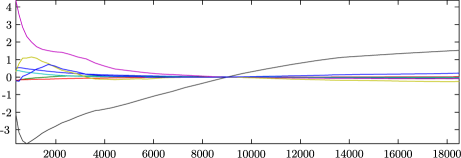
Figure 3: Parameter estimates for the covariance parameters in model F^′ for the ozone data as functions of the number of basis functions in the Hilbert space approximations.

4 Parameter estimation

In this section a parameter estimation procedure for the nested SPDE models is presented. One alternative would be to use a Metropolis–Hastings algorithm, which is easy to implement, but computationally inefficient. A better alternative is to use direct numerical optimization to estimate the parameters.

Let $Y(\mathbf{s})$ be an observation of the latent field, $X(\mathbf{s})$, given by (8) or (2.2), under mean zero Gaussian measurement noise, $\mathcal{E}(\mathbf{s})$, with variance $\sigma^{2}$:

$$Y(\mathbf{s})=X(\mathbf{s})+\mathcal{E}(\mathbf{s}).$$ (16)

Using the approximation procedure from Section 3, and assuming a regression model for the latent field’s mean value function, $\mu(\mathbf{s})$, the measurement equation can then be written as

$$\mathbf{Y}=\mathbf{M}\bolds{\mu}+\bolds{\Phi}\mathbf{w}+\bolds{\varepsilon},$$

where $\mathbf{M}$ is a matrix with the regression basis functions evaluated at the measurement locations, and $\bolds{\mu}$ is a vector containing the regression coefficients that have to be estimated. The matrix $\bolds{\Phi}$ contains the basis functions for the Hilbert space approximation procedure evaluated at the measurement locations, and $\mathbf{w}$ is the vector with the stochastic weights. In Section 3 it was shown that the vector $\mathbf{w}$ is Gaussian with mean zero and covariance matrix $\mathbf{H}\mathbf{Q}_{X_{0}}^{-1}\mathbf{H}^{\top}$. Both $\mathbf{Q}_{X_{0}}$ and $\mathbf{H}$ are sparse matrices, but neither the covariance matrix nor the precision matrix for $\mathbf{w}$ is sparse. Thus, it would seem as if one had to work with a dense covariance matrix, which would make maximum likelihood parameter estimation computationally infeasible for large data sets. However, because of the product form of the covariance matrix, one has that $\mathbf{w}=\mathbf{H}\mathbf{w}_{0}$, where $\mathbf{w}_{0}\sim\mathsf{N}_{C}(\mathbf{0},\mathbf{Q}_{X_{0}})$. Hence, the observation equation can be rewritten as

$$\mathbf{Y}=\mathbf{M}\bolds{\mu}+\bolds{\Phi}\mathbf{H}\mathbf{w}_{0}+\bolds{\varepsilon}.$$ (17)

Interpreting $\bolds{\Lambda}=\bolds{\Phi}\mathbf{H}$ as an observation matrix that depends on some of the parameters in the model, $\mathbf{Y}-\mathbf{M}\bolds{\mu}$ can now be seen as noisy observations of $\mathbf{w}_{0}$, which has a sparse precision matrix. The advantage with using (17) is that one then is in the setting of having observations of a latent Gaussian Markov random field, which facilitates the usage of sparse matrix techniques in the parameter estimation.

Let $\bolds{\psi}$ denote all parameters in the model except for $\bolds{\mu}$. Assuming that $\bolds{\mu}$ and $\bolds{\psi}$ are a priori independent, the posterior density can be written as

$$\pi(\mathbf{w}_{0},\bolds{\mu},\bolds{\psi}|\mathbf{Y})\propto\pi(\mathbf{Y}|\mathbf{w}_{0},\sigma^{2})\pi(\mathbf{w}_{0}|\bolds{\mu},\bolds{\psi})\pi(\bolds{\mu})\pi(\bolds{\psi}).$$

Using a Gaussian prior distribution with mean $\bolds{\mu}$ and precision $\mathbf{Q}_{\mu}$ for the mean parameters, the posterior distribution can be reformulated as

$$\pi(\mathbf{w}_{0},\bolds{\mu},\bolds{\psi}|\mathbf{Y})\propto\pi(\mathbf{w}_{0}|\bolds{\mu},\bolds{\psi},\mathbf{Y})\pi(\bolds{\mu}|\bolds{\psi},\mathbf{Y})\pi(\bolds{\psi}|\mathbf{Y}),$$ (18)

where $\mathbf{w}_{0}|\bolds{\mu},\bolds{\psi},\mathbf{Y}\sim\mathsf{N}_{C}(\mathbf{b},\hat{\mathbf{Q}})$, $\bolds{\mu}|\bolds{\psi},\mathbf{Y}\sim\mathsf{N}_{C}(\mathbf{b}_{\mu},\hat{\mathbf{Q}}_{\mu})$, and

$$\mathbf{b} = \frac{1}{\sigma^{2}}\bolds{\Lambda}^{\top}(\mathbf{Y}-\mathbf{M}\bolds{\mu}),\qquad\mathbf{b}_{\mu}=\mathbf{Q}_{\mu}\mathbf{m}_{\mu}+\frac{\mathbf{M}^{\top}\mathbf{Y}}{\sigma^{2}}-\frac{\mathbf{M}^{\top}\bolds{\Lambda}\hat{\mathbf{Q}}^{-1}\bolds{\Lambda}^{\top}\mathbf{Y}}{\sigma^{4}},$$

$$\hat{\mathbf{Q}} = \mathbf{Q}_{w_{0}}+\frac{1}{\sigma^{2}}\bolds{\Lambda}^{\top}\bolds{\Lambda},\qquad\hat{\mathbf{Q}}_{\mu}=\mathbf{Q}_{\mu}+\frac{\mathbf{M}^{\top}\mathbf{M}}{\sigma^{2}}-\frac{\mathbf{M}^{\top}\bolds{\Lambda}\hat{\mathbf{Q}}^{-1}\bolds{\Lambda}^{\top}\mathbf{M}}{\sigma^{4}}.$$

The calculations are omitted here since these expressions are calculated similarly to the posterior reformulation in Lindström and Lindgren (2008), which gives more computational details. Finally, the marginal posterior density $\pi(\bolds{\psi}|\mathbf{Y})$ can be shown to be

$$\pi(\bolds{\psi}|\mathbf{Y})\propto\frac{|\mathbf{Q}_{w_{0}}|^{{1/2}}\pi(\bolds{\psi})}{|\hat{\mathbf{Q}}|^{{1/2}}|\hat{\mathbf{Q}}_{\mu}|^{{1/2}}|\sigma\mathbf{I}|}\exp\biggl{(}\frac{1}{2\sigma^{2}}\mathbf{Y}^{\top}\biggl{(}\frac{\bolds{\Lambda}\hat{\mathbf{Q}}^{-1}\bolds{\Lambda}^{\top}}{\sigma^{2}}-\mathbf{I}\biggr{)}\mathbf{Y}+\frac{\mathbf{b}_{\mu}^{\top}\hat{\mathbf{Q}}_{\mu}^{-1}\mathbf{b}_{\mu}}{2}\biggr{)}.$$

By rewriting the posterior as (18), it can be integrated with respect to $\mathbf{w}_{0}$ and $\bolds{\mu}$, and instead of optimizing the full posterior with respect to $\mathbf{w}_{0}$, $\bolds{\mu}$ and $\bolds{\psi}$, only the marginal posterior $\pi(\bolds{\psi}|\mathbf{Y})$ has to be optimized with respect to $\bolds{\psi}$. This is a lower dimensional optimization problem, which substantially decreases the computational complexity. Given the optimum, $\bolds{\psi}_{\mathrm{opt}}=\operatorname{argmax}_{\bolds{\psi}}\pi(\bolds{\psi}|\mathbf{Y})$, $\bolds{\mu}_{\mathrm{opt}}$ is then given by $\bolds{\mu}_{\mathrm{opt}}=\hat{\mathbf{Q}}_{\mu}^{-1}\mathbf{b}_{\mu}$. In practice, the numerical optimization is carried out on $\log\pi(\bolds{\psi}|\mathbf{Y})$.

4.1 Estimating the parameter uncertainty

There are several ways one could estimate the uncertainty in the parameter estimates obtained by the parameter estimation procedure above. The simplest estimate of the uncertainty is obtained by numerically estimating the Hessian of the marginal posterior evaluated at the estimated parameters. The diagonal elements of the inverse of the Hessian can then be seen as estimates of the variance for the parameter estimates.

Another method for obtaining more reliable uncertainty estimates is to use a Metropolis–Hastings based MCMC algorithm with proposal kernel similar to the one used in Lindström and Lindgren (2008). A quite efficient algorithm is obtained by using random walk proposals for the parameters, where the correlation matrix for the proposal distribution is taken as a rescaled version of the inverse of the Hessian matrix [Gelman, Roberts and Gilks (1996)].

Finally, a third method for estimating the uncertainties is to use the INLA framework [Rue, Martino and Chopin (2009)], available as an R package (http://www.r-inla.org/). In settings with latent Gaussian Markov random fields, integrated nested Laplace approximations (INLA) provide close approximations to posterior densities for a fraction of the cost of MCMC. For models with Gaussian data, the calculated densities are for practical purposes exact. In the current implementation of the INLA package, handling the full nested SPDE structure is cumbersome, so further enhancements are needed before one can take full advantage of the INLA method for these models.

4.2 Computational complexity

In this section some details on the computational complexity for the parameter estimation and Kriging estimation are given.

The most widely used method for spatial prediction is linear Kriging. In the Bayesian setting, the Kriging predictor simply is the posterior expectation of the latent field $X$ given data and the estimated parameters. This expectation can be written as

$$\mathsf{E}(X|\bolds{\psi},\bolds{\mu},\mathbf{Y})=\mathbf{M}\bolds{\mu}+\bolds{\Phi}\mathbf{H}\mathsf{E}(\mathbf{w}_{0})=\mathbf{M}\bolds{\mu}+\bolds{\Phi}\mathbf{H}\hat{\mathbf{Q}}^{-1}\mathbf{b}.$$

The computationally demanding part of this expression is to calculate $\hat{\mathbf{Q}}^{-1}\mathbf{b}$. Since the $n\times n$ matrix $\mathbf{Q}$ is positive definite, this is most efficiently done using Cholesky factorization, forward substitution and back substitution: Calculate the Cholesky triangle $\mathbf{L}$ such that $\hat{\mathbf{Q}}=\mathbf{L}\mathbf{L}^{\top}$, and given $\mathbf{L}$, solve the linear system $\mathbf{L}\mathbf{x}=\mathbf{b}$. Finally, given $\mathbf{x}$, solve $\mathbf{L}^{\top}\mathbf{y}=\mathbf{x}$, where now $\mathbf{y}$ satisfies $\mathbf{y}=\hat{\mathbf{Q}}^{-1}\mathbf{b}$. Solving the forward substitution and back substitution are much less computationally demanding than calculating the Cholesky triangle. Hence, the computational cost for calculating the Kriging prediction is determined by the cost for calculating $\mathbf{L}$.

The computational complexity for the parameter estimation is determined by the optimization method that is used and the computational complexity for evaluating the marginal log-posterior $\log\pi(\bolds{\psi}|\mathbf{Y})$. The most computationally demanding terms in $\log\pi(\bolds{\psi}|\mathbf{Y})$ are the two log-determinants $\log|\mathbf{Q}_{w_{0}}|$ and $\log|\hat{\mathbf{Q}}|$ and the quadratic form $\mathbf{Y}^{\top}\bolds{\Lambda}\hat{\mathbf{Q}}^{-1}\bolds{\Lambda}\mathbf{Y}$, which are also most efficiently calculated using Cholesky factorization. Given the Cholesky triangle $\mathbf{L}$, the quadratic form can be obtained as $\mathbf{x}^{\top}\mathbf{x}$, where $\mathbf{x}$ is the solution to $\mathbf{L}\mathbf{x}=\bolds{\Lambda}\mathbf{Y}$, and the log-determinant $\log|\hat{\mathbf{Q}}|$ is simply the sum $2\sum_{i=1}^{n}\log\mathbf{L}_{ii}$. Thus, the computational cost for one evaluation of the marginal posterior is also determined by the cost for calculating $\mathbf{L}$. Because of the sparsity structure of $\hat{\mathbf{Q}}$, this computational cost is $\mathcal{O}(n)$, $\mathcal{O}(n^{3/2})$ and $\mathcal{O}(n^{2})$ for problems in one, two and three dimensions respectively [see Rue and Held (2005) for more details].

The computational complexity for the parameter estimation is highly dependent on the optimization method. If a Broyden–Fletcher–Goldfarb-Shanno (BFGS) procedure is used without an analytic expression for the gradients, the marginal posterior has to be evaluated $p$ times for each step in the optimization, where $p$ is the number of covariance parameters in the model. Thus, if $p$ is large and the initial value for the optimization is chosen far from the optimal value, many thousand evaluations of the marginal posterior may be needed in the optimization.

5 Application: Ozone data

On October 24, 1978, NASA launched the near-polar, Sun-synchronous orbiting satellite Nimbus-7. The satellite carried a TOMS instrument with the purpose of obtaining high-resolution global maps of atmospheric ozone [McPeters et al. (1996)]. The instrument measured backscattered solar ultraviolet radiation at 35 sample points along a line perpendicular to the orbital plane at 3-degree intervals from 51 degrees on the right side of spacecraft to 51 degrees on the left. A new scan was started every eight seconds, and as the measurements required sunlight, the measurements were made during the sunlit portions of the orbit as the spacecraft moved from south to north. The data measured by the satellite has been calibrated and preprocessed into a “Level 2” data set of spatially and temporally irregular Total Column Ozone (TCO) measurements following the satellite orbit. There is also a daily “Level 3” data set with values processed into a regular latitude-longitude grid. Both Level 2 and Level 3 data have been analyzed in recent papers in the statistical literature [Cressie and Johannesson (2008), Jun and Stein (2008), Stein (2007)].

In what follows, the nested SPDE models are used to obtain statistical estimates of a daily ozone map using a part of the Level 2 data. In particular, all data available for October 1st, 1988 is used, which is the same data set that was used by Cressie and Johannesson (2008).

5.1 Statistical model

The measurement model (16) is used for the ozone data. That is, the measurements, $Y(\mathbf{s})$, are assumed to be observations of a latent field of TCO ozone, $X(\mathbf{s})$, under Gaussian measurement noise $\mathcal{E}(\mathbf{s})$ with a constant variance $\sigma^{2}$. We let $X(\mathbf{s})$ have some mean value function, $\mu(\mathbf{s})$, and let the covariance structure be determined by a nested SPDE model. Inspired by Jun and Stein (2008), who proposed using differentiated Matérn fields for modeling TCO ozone, we use the simplest nested SPDE model. Thus, $Z(\mathbf{s})=X(\mathbf{s})-\mu(\mathbf{s})$ is generated by the system

$$\bigl{(}\kappa^{2}(\mathbf{s})-\Delta\bigr{)}Z_{0}(\mathbf{s}) = \mathcal{W}(\mathbf{s})$$

$$Z(\mathbf{s}) = \bigl{(}b(\mathbf{s})+\mathbf{B}(\mathbf{s})^{\top}\nabla\bigr{)}Z_{0}(\mathbf{s}),$$

where $\mathcal{W}(\mathbf{s})$ is Gaussian white noise on the sphere. If $\kappa(\mathbf{s})$ is assumed to be constant, the ozone is modeled as a Gaussian field with a covariance structure that is obtained by applying the differential operator $(b(\mathbf{s})+\mathbf{B}(\mathbf{s})^{\top}\nabla)$ to a stationary Matérn field, which is similar to the model by Jun and Stein (2008). If, on the other hand, $\kappa$ is spatially varying, the range of the Matérn-like covariance function can vary with location. As in Stein (2007) and Jun and Stein (2008), the mean can be modeled using a regression basis of spherical harmonics; however, since the data set only contains measurements from one specific day, it is not possible to identify which part of the variation in the data that comes from a varying mean and which part that can be explained by the variance–covariance structure of the latent field. To avoid this identifiability problem, $\mu(\mathbf{s})$ is assumed to be unknown but constant. The parameter $\kappa^{2}(\mathbf{s})$ has to be positive, and for identifiability reasons, we also require $b(\mathbf{s})$ to be positive. We, therefore, let $\log\kappa^{2}(\mathbf{s})=\sum_{k,m}\kappa_{k,m}Y_{k,m}(\mathbf{s})$ and $\log b(\mathbf{s})=\sum_{k,m}b_{k,m}Y_{k,m}(\mathbf{s})$, where $Y_{k,m}$ is the spherical harmonic of order $k$ and mode $m$. Finally, the vector field $\mathbf{B}(\mathbf{s})$ is modeled using the vector spherical harmonics basis functions $\Upsilon_{k,m}^{1}$ and $\Upsilon_{k,m}^{2}$, presented in Appendix:

$$\mathbf{B}(\mathbf{s})=\sum_{k,m}\bigl{(}B_{k,m}^{1}\Upsilon_{k,m}^{1}(\mathbf{s})+B_{k,m}^{2}\Upsilon_{k,m}^{2}(\mathbf{s})\bigr{)}.$$

Table 1: Maximal orders of the spherical harmonics used in the bases for the different parameters and total number of covariance parameters in the different models for $X(\mathbf{s})$

	A	B	C	D	E	F	G	H	I	J	K	L	M
$\kappa^{2}(\mathbf{s})$	0	1	00	01	02	00	03	02	00	04	03	00	04
$b(\mathbf{s})$	0	1	01	01	02	02	03	02	03	04	03	04	04
$\mathbf{B}(\mathbf{s})$	0	0	01	01	00	02	00	02	03	00	03	04	04
Total	2	8	11	14	18	26	32	34	47	50	62	75	98

[]Notes: The actual number of basis functions for $\kappa^{2}(\mathbf{s})$ and $b(\mathbf{s})$ are given by $(\mathit{ord}+1)^{2}$, and for $\mathbf{B}(\mathbf{s})$, the actual number is $2(\mathit{ord}+1)^{2}-2$, where $\mathit{ord}$ is the maximal order indicated in the table.

To choose the number of basis functions for the parameters $\kappa^{2}(\mathbf{s})$, $b(\mathbf{s})$ and $\mathbf{B}(\mathbf{s})$, some model selection technique has to be used. Model selection for this model class is difficult since the models can have both nonstationary mean value functions and nonstationary covariance structures. This makes standard variogram techniques inadequate in general, and we instead base the model selection on Akaike’s Information Criterion (AIC) and the Bayesian Information Criterion (BIC) [Hastie, Tibshirani and Friedman (2001)], which are suitable model selection tools for the nested SPDE models since the likelihood for the data can be evaluated efficiently.

We estimate 13 models with different numbers of covariance parameters, presented in Table 1. The simplest model is a stationary Matérn model, with four parameters to estimate, and the most complicated model has $100$ parameters to estimate, including the mean and the measurement noise variance. There are three different types of models in Table 1: In the first type (models B, E, G and J), $\kappa^{2}$ and $b$ are spatially varying and the vector field $\mathbf{B}$ is assumed to be zero. In the second type (models C, F, I and L), $b$ and $\mathbf{B}$ are spatially varying and $\kappa^{2}$ is assumed to be constant. Finally, in the third type (model D, H, K and M), all parameters are spatially varying.

A basis of 9002 piecewise linear functions induced by a triangulation of the Earth (see Figure 4) is used in the approximation procedure from Section 3 to get efficient representations of each model, and the parameters are estimated using the procedure from Section 4. The computational cost for the parameter estimation only depends on the number of basis functions in the Hilbert space approximation, and not on the number of data points, which makes inference efficient even for this large data set.

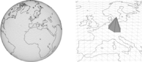
Figure 4: The left part shows the triangulation of the Earth used to define the piecewise linear basis functions in the Hilbert space approximation for ozone data. Each basis function is one at a node in the triangulation, and decreases linearly to zero at the neighboring nodes. The right part of the figure shows one of these functions.

Figure 5: AIC (squares) and BIC (circles) for the models A–M (solid lines) and the axially symmetric models A^′–M^′ (dashed lines), scaled by a factor $10^{-5}$. Note that the major improvement in AIC and BIC occurs when the orders of the basis functions are increased from one to two, and that the model type with spatially varying $b$ and $\mathbf{B}$ seems to be most appropriate for this data. Also note that the axially symmetric model F^′ is surprisingly good considering that it only has $8$ covariance parameters.

AIC and BIC for each of the fitted models can be seen in Figure 5. The figure contains one panel for each of the three model types and one panel where AIC and BIC are shown for all models at once. The major improvement in AIC and BIC occurs when the orders of the basis functions are increased from one to two. For the first model type, with spatially varying $\kappa^{2}$ and $b$, the figure indicates that the results could be improved by increasing the orders of the basis functions further. However, for a given order of the basis functions, the other two model types have much lower AIC and BIC. Also, by comparing AIC and BIC for the second and third model types, one finds that there is not much gain in letting $\kappa^{2}$ be spatially varying. We therefore conclude that a model with spatially varying $b$ and $\mathbf{B}$ is most appropriate for this data.

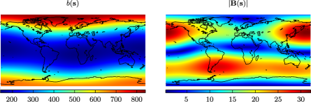
Figure 6: Estimated variance-scaling parameter, $b(\mathbf{s})$, and the the norm of the vectors in the estimated vector field $\mathbf{B}(\mathbf{s})$ for model F. Note that the estimates are fairly constant with respect to longitude, which indicates that the latent field could be axially symmetric.

The estimated parameters $b(\mathbf{s})$ and the length of the vectors $\mathbf{B}(\mathbf{s})$ for model F are shown in Figure 6. One thing to note in this figure is that the two parameters are fairly constant with respect to longitude, which indicates that the latent field could be axially symmetric, an assumption that was made by both Stein (2007) and Jun and Stein (2008). If the latent field indeed was axially symmetric, one would only need the basis functions that are constant with respect to longitude in the parameter bases. Since there is only one axially symmetric spherical harmonic for each order, this assumption drastically reduces the number of parameters for the models in Table 1. Let A^′–M^′ denote the axially symmetric versions of models A–M. For these models, the number of basis functions for both $\kappa^{2}(\mathbf{s})$ and $b(\mathbf{s})$ is $\mathit{ord}+1$, and the number of basis functions for $\mathbf{B}(\mathbf{s})$ is $2(\mathit{ord}+1)-2$, where $\mathit{ord}$ is the maximal order indicated in Table 1. The dashed lines in Figure 5 show AIC and BIC calculated for these models. Among the axially symmetric models, model F^′ is surprisingly good considering that it only has $8$ covariance parameters.

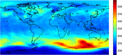
Figure 7: Kriging estimate of TCO ozone in Dobson units using model F^′.

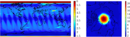
Figure 8: Standard error in Dobson units for the Kriging estimate. The color bar in the left part of the figure has been truncated at 6 Dobson units. The behavior near the north pole can be seen in the right part of the figure.

The Kriging estimate and its standard error for model F^′ are shown in Figures 7 and 8 respectively. The oscillating behavior near the equator for the standard error is explained by the fact that the satellite tracks are furthest apart there, which results in sparser measurements between the different tracks. Because the measurements are collected using backscattered sunlight, the variance close to the north pole is high, as there are no measurements there. As seen in Figure 9, there is not much spatial correlation in the residuals $\hat{\mathbf{X}}-\mathbf{Y}$, which indicates a good model fit. In Figure 10, estimates of the local mean and variance of the residuals are shown. The mean is fairly constant across the globe, but there is a slight tendency for higher variance closer to the poles. This is due to the fact that the data really is space–time data, as the measurements are collected during a 24-hour period. Since the different satellite tracks are closest near the poles, the temporal variation of the data is most prominent here, and especially near the international date line where data is collected both at the first satellite track of the day and at the last track, 24 hours later. The area with high residual variance is one of those places where measurements are taken both at the beginning and the end of the time period, and where the ozone concentration has changed during the time period between the measurements. One could include this effect by allowing the variance of the measurement noise to be spatially varying; however, one should really use a spatio-temporal model for the data to correctly account for the effect, which is outside the scope of this article.

Table 2: Estimates of the covariance parameters in model F^′ using all data but the first track ($Y_{f}$), all data but the last track ($Y_{l}$), and all data ($Y$)

	$\bolds{\kappa}$	$\bolds{\sigma}$	$\bolds{b_{1}}$	$\bolds{b_{2}}$	$\bolds{b_{3}}$	$\bolds{B_{1}}$	$\bolds{B_{2}}$	$\bolds{B_{3}}$	$\bolds{B_{4}}$
$Y_{f}$	$0.74$	$25.60$	$5.85$	$0.045$	$0.34$	$1.05$	$2.59$	$-6.84$	$-0.84$
$Y_{l}$	$0.73$	$25.56$	$5.82$	$0.033$	$0.34$	$0.90$	$2.38$	$-7.01$	$-0.82$
$Y$	$0.67$	$34.09$	$5.75$	$0.054$	$0.36$	$0.70$	$2.48$	$-7.10$	$-0.68$

Figure 9: Estimated covariance function for the Kriging residuals using model F^′.

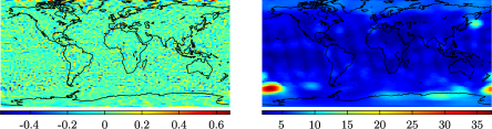
Figure 10: Estimates of the local mean (left) and standard deviation (right) for the Kriging residuals using model F^′. The mean is fairly constant across the globe, whereas the standard deviation is higher close to the poles and at the international date line because of the temporal structure in the data.

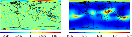
Figure 11: The ratio between the kriging estimates using model F^′ and model M (left), and the ratio between the corresponding kriging standard errors (right). Note that there is not much difference between the Kriging estimates, whereas there is a clear difference between the corresponding standard errors.

To see how much the temporal structure near the international date line influences the model fit, the parameters in model F^′ are re-estimated without using the first satellite track of the day and without using the last track of the day. The estimated parameters can be seen in Table 2 and, as expected, the estimate of the measurement noise variance is much lower when not using all date line data. The estimates of the covariance parameters for the latent field also change somewhat, but the large scale structure of the nonstationarity is preserved.

To study how sensitive the Kriging estimates are to the model choice, the ratio between the Kriging estimates for the simple model F^′ and the large model M, and the ratio between the corresponding Kriging standard errors, are shown in Figure 11. There is not much difference between the two Kriging estimates, whereas there is a clear difference between the corresponding standard errors. Thus, if one only is interested in the Kriging estimate, it does not matter much which model is used, but if one also is interested in the standard error of the estimate, the model choice greatly influences the results.

5.2 Discussion

Before the nested SPDE models were used on the ozone data, several tests were performed on simulated data to verify that the model parameters in fact could be estimated using the estimation procedure in Section 4. These tests showed that the estimation procedure is robust given that the initial values for the parameters are not chosen too far from the true values. However, for nonstationary models with many covariance parameters, it is not easy to choose the initial values. To reduce this problem, the optimization is done in several steps. A stationary Matérn model (model A) is estimated to get initial values for $\kappa_{0,0}$, $b_{0,0}$ and $\sigma^{2}$. To estimate model B, all parameters are set to zero initially, except for the parameters that were estimated in model A. Another layer of spherical harmonics is added to the bases for $\kappa^{2}(\mathbf{s})$ and $b(\mathbf{s})$ for estimating model E using the model B parameters as initial values. This step-wise procedure of adding layers of spherical harmonics to the bases is then repeated to estimate the larger models. Numerical studies showed that this optimization procedure is quite robust even for large models; however, as in most other numerical optimization problems, there are no guarantees that the true optimal values have been found for all models for the ozone data.

The application of the nested SPDE models to ozone data was inspired by Jun and Stein (2008), who proposed using differentiated Matérn fields for modeling TCO ozone, and we conclude this section with some remarks on the similarities and differences between the nested SPDEs and their models. The most general model in Jun and Stein (2008) is on the form

$$X(\mathbf{s}) = P_{1}(l_{2})X_{0}(\mathbf{s})+\biggl{(}P_{2}(l_{2})\frac{\partial}{\partial l_{2}}+P_{3}(l_{2})\frac{\partial}{\partial l_{1}}\biggr{)}X_{1}(\mathbf{s})$$

$${}+P_{4}(l_{2})\frac{\partial}{\partial l_{1}}X_{2}(\mathbf{s}),$$

where $X_{i},i=0,1,2$, are i.i.d. Matérn fields in $\mathbb{R}^{3}$, $P_{i},i=1,2,3,4$, are nonrandom functions depending on latitude, $l_{1}$ denoted longitude and $l_{2}$ denoted latitude. This model is similar to the model used here, but there are some important differences. First of all, (5.2) contains a sum of three independent fields, which we cannot represent since the approximation procedure in Section 3 in this case loses its computational benefits. To get a model more similar to the nested SPDE model, one would have to let $P_{4}(l_{2})\equiv 0$, and $X_{0}(\mathbf{s})=X_{1}(\mathbf{s})$. Using $X_{0}=X_{1}$ or $X_{0}$ and $X_{1}$ as i.i.d. copies of a Matérn field gives different covariance functions, and without testing both cases it is hard to determine what is more appropriate for ozone data.

Another important conceptual difference is how the methods deal with the spherical topology. The Matérn fields in Jun and Stein (2008) are stochastic fields on $\mathbb{R}^{3}$, evaluated on the embedded sphere, which is equivalent to using chordal distance as the metric in a regular Matérn covariance function. One might instead attempt to evaluate the covariance function using the arc-length distance, which is a more natural metric on the sphere. However, Theorem 2 from Gneiting (1998) shows that for Matérn covariances with $\nu\geq 1$, this procedure does not generate positive definite covariance functions. This means that the arc-length method cannot be used for any differentiable Matérn fields. On the other hand, the nested SPDEs are directly defined on the sphere, and therefore inherently use the arc-length distance.

There is, in theory, no difference between writing the directional derivative of $X(\mathbf{s})$ as $(P_{2}(l_{2})\frac{\partial}{\partial l_{2}}+P_{3}(l_{2})\frac{\partial}{\partial l_{1}})X_{1}(\mathbf{s})$ or $\mathbf{B}(\mathbf{s})^{\top}\nabla X(\mathbf{s})$, but the latter is easier to work with in practice. If a vector field basis is used to model $\mathbf{B}(s)$, the process will not have any singularities as long as the basis functions are nonsingular, which is the case for the basis used in this paper. If, on the other hand, $P_{2}(l_{2})$ and $P_{3}(l_{2})$ are modeled separately, the process will be singular at the poles unless certain restrictions on the two functions are met. This fact is indeed noted by Jun and Stein (2008), but the authors do not seem to take the restrictions into account in the parameter estimation, which causes all their estimated models to have singularities at the poles.

Finally, the nested SPDE models are computationally efficient also for spatially irregular data, which allowed us to work with the TOMS Level 2 data instead of the gridded Level 3 data.

6 Concluding remarks

There is a need for computationally efficient stochastic models for environmental data. Lindgren, Rue and Lindström (2010) introduced an efficient procedure for obtaining Markov approximations of, possibly nonstationary, Matérn fields by considering Hilbert space approximations of the SPDE

$$\bigl{(}\kappa(\mathbf{s})^{2}-\Delta\bigr{)}^{{\alpha/2}}X(\mathbf{s})=\phi(\mathbf{s})\mathcal{W}(\mathbf{s}).$$

In this work, the class of nonstationary nested SPDE models generated by (2.2) was introduced, and it was shown how the approximation methods in Lindgren, Rue and Lindström (2010) can be extended to this larger class of models. This model class contains a wider family of covariance models, including both Matérn-like covariance functions and various oscillating covariance functions. Because of the additional differential operator $\mathcal{L}_{2}$, the Hilbert space approximations for the nested SPDE models do not have the Markov structure the model in Lindgren, Rue and Lindström (2010) has, but all computational benefits from the Markov properties are preserved for the nested SPDE models using the procedure in Section 4. This allows us to fit complicated models with over 100 parameters to data sets with several hundred thousand measurements using only a standard personal computer.

By choosing $\mathcal{L}_{2}=b+\mathbf{B}^{\top}\nabla$, one obtains a model similar to what Jun and Stein (2008) used to analyze TOMS Level 3 ozone data, and we used this restricted nested SPDE model to analyze the global spatially irregular TOMS Level 2 data. This application illustrates the ability to use the model class to produce nonstationary covariance models on general smooth manifolds which efficiently can be used to study large spatially irregular data sets.

The most important next step in this work is to make a spatio-temporal extension of the model class. This would allow us to produce not only spatial but also spatio-temporal ozone models and increase the applicability of the model class to other environmental modeling problems where time dependence is a necessary model component.

Appendix: Vector spherical harmonics

When using the nonstationary model (2.2) in practice, we assume that the parameters in the model can be expressed in terms of some basis functions. If working on the sphere, spherical harmonics is a convenient basis for the parameters taking values in $\mathbb{R}$. On real form, the spherical harmonic $Y_{k,m}(\mathbf{s})$ of order $k\in\mathbb{N}_{0}$ and mode $m=-k,\ldots,k$ is defined as

$$\ Y_{k,m}(\mathbf{s})=\sqrt{\frac{2k+1}{4\pi}\cdot\frac{(k-|m|)!}{(k+|m|)!}}\cdot\cases{\sqrt{2}\sin(ml_{1})P_{k,-m}(\sin l_{2}),&\quad$-k\leq m<0,$\cr P_{k,0}(\sin l_{2}),&\quad$m=0,$\cr\sqrt{2}\cos(ml_{1})P_{k,m}(\sin l_{2}),&\quad$0<m\leq k,$}$$

where $l_{2}$ is the latitude, $l_{1}$ is the longitude, and $P_{k,m}(\cdot)$ are associated Legendre functions. We, however, also need a basis for the vector fields $\mathbf{B}_{i}(\mathbf{s})$, determining the direction and magnitude of differentiation. Since the vector fields in each point on the sphere must lie in the tangent space of $\mathbb{S}^{2}$, the basis functions also must satisfy this. A basis with this property is obtained by using a subset of the vector spherical harmonics [Hill (1954)]. For each spherical harmonic $Y_{k,m}(\mathbf{s})$, $k>0$, define the two vector spherical harmonics

$$\Upsilon_{k,m}^{1}(\mathbf{s}) = \nabla_{\mathbb{S}^{2}}Y_{k,m}(\mathbf{s}),$$

$$\Upsilon_{k,m}^{2}(\mathbf{s}) = \nabla_{\mathbb{S}^{2}}Y_{k,m(\mathbf{s})}\times\mathbf{s}.$$

Here $\times$ denotes the cross product in $\mathbb{R}^{3}$ and $\nabla_{\mathbb{S}^{2}}$ is the gradient on $\mathbb{S}^{2}$. By defining the basis in this way, all basis functions in $\Upsilon^{1}=\{\Upsilon_{k,m}^{1}\}$ and $\Upsilon^{2}=\{\Upsilon_{k,m}^{2}\}$ will obviously lie in the tangent space of $\mathbb{S}^{2}$. It is also easy to see that the basis is orthogonal in the sense that for any $k,l>0$, $-k\leq m\leq k$, and $-l\leq n\leq l$, one has

$$\langle{\Upsilon_{k,m}^{1}},{\Upsilon_{l,n}^{2}}\rangle_{\mathbb{S}^{2}} = 0,$$

$$\langle{\Upsilon_{k,m}^{1}},{\Upsilon_{l,n}^{1}}\rangle_{\mathbb{S}^{2}} = k(k+1)\delta_{k-l}\delta_{m-n},$$

$$\langle{\Upsilon_{k,m}^{2}},{\Upsilon_{l,n}^{2}}\rangle_{\mathbb{S}^{2}} = k(k+1)\delta_{k-l}\delta_{m-n}.$$

These are indeed desirable properties for a vector field basis, but for the basis to be of any use in practice, a method for calculating the basis functions explicitly is needed. Such explicit expressions are given in the following proposition.

Proposition .1

With $\mathbf{s}=(x,y,z)^{\top}$, $\Upsilon_{k,m}^{1}(\mathbf{s})$ and $\Upsilon_{k,m}^{2}(\mathbf{s})$ can be written as

$$\Upsilon_{k,m}^{1}(\mathbf{s}) = \frac{1}{1-z^{2}}\left[\matrix{-myY_{k,-m}(\mathbf{s})-c_{k,m}xzY_{k-1,m}(\mathbf{s})+kxz^{2}Y_{k,m}(\mathbf{s})\cr mxY_{k,-m}(\mathbf{s})-c_{k,m}yzY_{k-1,m}(\mathbf{s})+kyz^{2}Y_{k,m}(\mathbf{s})\cr c_{k,m}(1-z^{2})Y_{k-1,m}(\mathbf{s})-(1-z^{2})kzY_{k,m}(\mathbf{s})}\right],$$

$$\Upsilon_{k,m}^{2}(\mathbf{s}) = \frac{1}{1-z^{2}}\left[\matrix{kzyY_{k,m}(\mathbf{s})-c_{k,m}yY_{k-1,m}(\mathbf{s})+mzxY_{k,-m}(\mathbf{s})\cr-kxzY_{k,m}(\mathbf{s})+c_{k,m}xY_{k-1,m}(\mathbf{s})+myzY_{k,-m}(\mathbf{s})\cr-m(1-z^{2})Y_{k,-m}(\mathbf{s})}\right],$$

where

$$c_{k,m}=\sqrt{\frac{(2k+1)(k^{2}-|m|^{2})}{2k-1}}.$$

One has that $\nabla_{\mathbb{S}^{2}}Y_{k,m}=P_{\mathbb{S}^{2}}(\nabla_{\mathbb{R}^{3}}Y_{k,m})$, that is, the gradient on $\mathbb{S}^{2}$ can be obtained by first calculating the gradient in $\mathbb{R}^{3}$ and then projecting the result onto $\mathbb{S}^{2}$. If $c_{k}^{m}$ denotes the normalization constant for the spherical harmonic $Y_{k,m}(\mathbf{s})$, and the recursive relation

$$(1-z^{2})\frac{\partial}{\partial z}P_{k,m}(z)=kzP_{k,m}(z)-(k+m)P_{k-1,m}(z)$$

is used, one has that

$$\frac{\partial}{\partial z}Y_{k,m}(\mathbf{s})=\frac{1}{1-z^{2}}\biggl{(}kzY_{k,m}(\mathbf{s})-(k+|m|)\frac{c_{k}^{m}}{c_{k-1}^{m}}Y_{k-1,m}(\mathbf{s})\biggr{)}.$$

Now, using that $\tan(l_{1})=x^{-1}y$, one has

$$\frac{\partial l_{1}}{\partial x} = -\cos^{2}(l_{1})\frac{y}{x^{2}}=-\frac{y}{1-z^{2}},$$

$$\frac{\partial l_{1}}{\partial y} = \cos^{2}(l_{1})\frac{1}{x}=\frac{x}{1-z^{2}},$$

where the last equalities hold on $\mathbb{S}^{2}$. Using these relations gives

$$\frac{\partial}{\partial x}Y_{k,m}(\mathbf{s})=-\frac{my}{1-z^{2}}Y_{k,-m}(\mathbf{s}),\qquad\frac{\partial}{\partial y}Y_{k,m}(\mathbf{s})=\frac{mx}{1-z^{2}}Y_{k,-m}(\mathbf{s}).$$

Thus, with

$$c_{k,m}\mathrel{\triangleq}(k+|m|)\frac{c_{k}^{m}}{c_{k-1}^{m}}=\sqrt{\frac{(2k+1)(k^{2}-|m|^{2})}{2k-1}},$$

one has that

$$\nabla_{\mathbb{R}^{3}}Y_{k,m}(\mathbf{s})=\frac{1}{1-z^{2}}\left[\matrix{-myY_{k,-m}(\mathbf{s})\cr mxY_{k,-m}(\mathbf{s})\cr kzY_{k,m}(\mathbf{s})-c_{k,m}Y_{k-1,m}(\mathbf{s})}\right].$$

Finally, the desired result is obtained by calculating

$$\Upsilon_{k,m}^{1} = \nabla_{\mathbb{S}^{2}}Y_{k,m}=\mathbf{P}_{\mathbb{S}^{2}}\nabla_{\mathbb{R}^{3}}Y_{k,m},$$

$$\Upsilon_{k,m}^{2} = \Upsilon_{k,m}^{1}\times\mathbf{s}=\mathbf{S}_{\times}\Upsilon_{k,m}^{1},$$

where

$$\mathbf{P}_{\mathbb{S}^{2}}=(I-\mathbf{s}\mathbf{s}^{\top})=\left[\matrix{1-x^{2}&-xy&-xz\cr-xy&1-y^{2}&-yz\cr-xz&-yz&1-z^{2}}\right],\qquad\mathbf{S}_{\times}=\left[\matrix{0&-z&y\cr z&0&-x\cr-y&x&0}\right].$$

References

- Adler (1981) {bbook}[author] \bauthor\bsnmAdler, \bfnmR. J.\binitsR. J. (\byear1981). \btitleThe Geometry of Random Fields. \bpublisherWiley, New York. \MR0611857 \endbibitem
- Bolin and Lindgren (2009) {barticle}[author] \bauthor\bsnmBolin, \bfnmD.\binitsD. and \bauthor\bsnmLindgren, \bfnmF.\binitsF. (\byear2009). \btitleWavelet Markov approximations as efficient alternatives to tapering and convolution fields (submitted). \bmiscPreprints in \bjournalMath. Sci. \banumber2009:13, \bmiscLund Univ. \endbibitem
- Cressie and Johannesson (2008) {barticle}[author] \bauthor\bsnmCressie, \bfnmNoel\binitsN. and \bauthor\bsnmJohannesson, \bfnmGardar\binitsG. (\byear2008). \btitleFixed rank kriging for very large spatial data sets. \bjournalJ. R. Stat. Soc. Ser. B Stat. Methodol. \bvolume70 \bpages209–226. \MR2412639 \endbibitem
- Gelman, Roberts and Gilks (1996) {barticle}[author] \bauthor\bsnmGelman, \bfnmA.\binitsA., \bauthor\bsnmRoberts, \bfnmG. O.\binitsG. O. and \bauthor\bsnmGilks, \bfnmW. R.\binitsW. R. (\byear1996). \btitleEfficient Metropolis jumping rules. \bjournalBayesian Stat. \bvolume5 \bpages599–607. \MR1425429 \endbibitem
- Gneiting (1998) {barticle}[author] \bauthor\bsnmGneiting, \bfnmT\binitsT. (\byear1998). \btitleSimple tests for the validity of correlation function models on the circle. \bjournalStatist. Probab. Lett. \bvolume39 \bpages119–122. \MR1652540 \endbibitem
- Hastie, Tibshirani and Friedman (2001) {bbook}[author] \bauthor\bsnmHastie, \bfnmT.\binitsT., \bauthor\bsnmTibshirani, \bfnmR.\binitsR. and \bauthor\bsnmFriedman, \bfnmJ. H.\binitsJ. H. (\byear2001). \btitleThe Elements of Statistical Learning. \bpublisherSpringer, \baddressNew York. \MR1851606 \endbibitem
- Hill (1954) {barticle}[author] \bauthor\bsnmHill, \bfnmE. L.\binitsE. L. (\byear1954). \btitleThe theory of vector spherical harmonics. \bjournalAmer. J. Phys. \bvolume22 \bpages211–214. \MR0061226 \endbibitem
- Jun and Stein (2007) {barticle}[author] \bauthor\bsnmJun, \bfnmMikyoung\binitsM. and \bauthor\bsnmStein, \bfnmMichael L.\binitsM. L. (\byear2007). \btitleAn approach to producing space–time covariance functions on spheres. \bjournalTechnometrics \bvolume49 \bpages468–479. \MR2394558 \endbibitem
- Jun and Stein (2008) {barticle}[author] \bauthor\bsnmJun, \bfnmMikyoung\binitsM. and \bauthor\bsnmStein, \bfnmMichael L.\binitsM. L. (\byear2008). \btitleNonstationary covariance models for global data. \bjournalAnn. Appl. Statist. \bvolume2 \bpages1271–1289. \endbibitem
- Lindgren, Rue and Lindström (2010) {barticle}[author] \bauthor\bsnmLindgren, \bfnmFinn\binitsF., \bauthor\bsnmRue, \bfnmHávard\binitsH. and \bauthor\bsnmLindström, \bfnmJohan\binitsJ. (\byear2010). \btitleAn explicit link between Gaussian fields and Gaussian Markov random fields, The SPDE approach (submitted). \bmiscPreprints in \bjournalMath. Sci. \banumber2010:3, \bmiscLund Univ. \endbibitem
- Lindström and Lindgren (2008) {barticle}[author] \bauthor\bsnmLindström, \bfnmJohan\binitsJ. and \bauthor\bsnmLindgren, \bfnmFinn\binitsF. (\byear2008). \btitleA Gaussian Markov random field model for total yearly precipitation over the African Sahel. \bmiscPreprints in \bjournalMath. Sci. \banumber2008:8, \bmiscLund Univ. \endbibitem
- Matérn (1960) {bbook}[author] \bauthor\bsnmMatérn, \bfnmB.\binitsB. (\byear1960). \btitleSpatial Variation. \bpublisherMeddelanden från statens skogsforskningsinstitut, Stockholm. \endbibitem
- McPeters et al. (1996) {barticle}[author] \bauthor\bsnmMcPeters, \bfnmR. D.\binitsR. D., \bauthor\bsnmBhartia, \bfnmP. K.\binitsP. K., \bauthor\bsnmKrueger, \bfnmA. J.\binitsA. J., \bauthor\bsnmHerman, \bfnmJ. R.\binitsJ. R., \bauthor\bsnmSchlesinger, \bfnmB.\binitsB., \bauthor\bsnmWellemeyer, \bfnmC. G.\binitsC. G., \bauthor\bsnmSeftor, \bfnmC. J.\binitsC. J., \bauthor\bsnmJaross, \bfnmG.\binitsG., \bauthor\bsnmTaylor, \bfnmS. L.\binitsS. L., \bauthor\bsnmSwissler, \bfnmT.\binitsT., \bauthor\bsnmTorres, \bfnmO.\binitsO., \bauthor\bsnmLabow, \bfnmG.\binitsG., \bauthor\bsnmByerly, \bfnmW.\binitsW. and \bauthor\bsnmCebula, \bfnmR. P.\binitsR. P. (\byear1996). \btitleNimbus-7 Total Ozone Mapping Spectrometer (TOMS) data products user’s guide. \bmiscNASA Reference Publication 1384. \endbibitem
- Rue and Held (2005) {bbook}[author] \bauthor\bsnmRue, \bfnmH.\binitsH. and \bauthor\bsnmHeld, \bfnmL.\binitsL. (\byear2005). \btitleGaussian Markov Random Fields. \bpublisherChapman & Hall/CRC, \baddressBoca Raton, FL. \MR2130347 \endbibitem
- Rue, Martino and Chopin (2009) {barticle}[author] \bauthor\bsnmRue, \bfnmH\binitsH., \bauthor\bsnmMartino, \bfnmS\binitsS. and \bauthor\bsnmChopin, \bfnmN\binitsN. (\byear2009). \btitleApproximate Bayesian inference for latent Gaussian models using integrated nested laplace approximations (with discussion). \bjournalJ. R. Stat. Soc. Ser. B Stat. Methodol. \bvolume71 \bpages319–392. \endbibitem
- Stein (2007) {barticle}[author] \bauthor\bsnmStein, \bfnmMichael L.\binitsM. L. (\byear2007). \btitleSpatial variation of total column ozone on a global scale. \bjournalAnn. Appl. Statist. \bvolume1 \bpages191–210. \MR2393847 \endbibitem
- Thomas and Finney (1995) {bbook}[author] \bauthor\bsnmThomas, \bfnmG. B.\binitsG. B. and \bauthor\bsnmFinney, \bfnmR. L.\binitsR. L. (\byear1995). \btitleCalculus and Analytic Geometry, \bedition9 ed. \bpublisherAddison Wesley, \baddressNew York. \endbibitem
- Whittle (1963) {barticle}[author] \bauthor\bsnmWhittle, \bfnmP.\binitsP. (\byear1963). \btitleStochastic processes in several dimensions. \bjournalBull. Inst. Internat. Statist. \bvolume40 \bpages974–994. \MR0173287 \endbibitem
- Yaglom (1987) {bbook}[author] \bauthor\bsnmYaglom, \bfnmA. M.\binitsA. M. (\byear1987). \btitleCorrelation Theory of Stationary and Related Random Functions \bvolume1. \bpublisherSpringer, \baddressNew York. \endbibitem