Effective medium theory for superconducting layers: A systematic analysis including space correlation effects

Abstract

We investigate the effects of mesoscopic inhomogeneities on the metal-superconductor transition occurring in several two-dimensional electron systems. Specifically, as a model of systems with mesoscopic inhomogeneities, we consider a random-resistor network, which we solve both with an exact numerical approach and by the effective medium theory. We find that the width of the transition in these two-dimensional superconductors is mainly ruled by disorder rather than by fluctuations. We also find that “tail” features in resistivity curves of interfaces between LaAlO₃ or LaTiO₃ and SrTiO₃ can arise from a bimodal distribution of mesoscopic local $T_{c}$’s and/or substantial space correlations between the mesoscopic domains.

I Introduction

The recent discovery of superconductivity in transition metal oxide interfacesreyren ; triscone ; espci and of pseudogap effects and disordered-induced inhomogeneity in thin conventional superconducting filmssacepe1 ; sacepe2 ; sacepe3 ; mondal has triggered a renewed interest in transport and superconductivity in two-dimensional electronic systems.review_feigelman Owing to their low dimensionality and to unavoidable defects in the growing processes, disorder plays an important role in the physics of these systems. First of all, impurities lead to localization effects, which can degrade the superconducting critical temperaturefinkelstein and can give rise to localized preformed Cooper pairs.leema ; feigelman ; dubi ; randeria As it has become evident in a number of recent numerical works,dubi ; randeria the system manifests a spontaneous tendency towards inhomogeneities even in the presence of a homogenous disorder distribution. In particular disorder can also give rise to patchy electronic systems which are inhomogeneous on a mesoscopic scale, with superconducting regions embedded in, or connected by, normal/insulating regions.ioffe ; feigelman10 ; review_feigelman

Understanding all such issues is a difficult task, particularly close to the superconductor-insulator transition, and it would obviously involve together concepts like percolation, establishment of coherence between superconducting “islands”, role of disorder in the Berezinski-Kosterlitz-Thouless transition, and so on. In this context it would be useful to disentangle the various aspects by understanding whether and which properties of these systems could be explained just in terms of mesoscopic inhomogeneities. Therefore we find it important and timely to investigate systematically the effects of large scale inhomogeneities on the superconducting transition in two dimension, irrespectively of their microscopic origin. The analysis of these effects seems particularly compelling in metal-oxide interfaces, upon inspecting their sheet resistance $R_{\square}(T)$ data around the critical temperature. While homogeneously disordered films of conventional superconductors present rather sharp transitions with high slopes of $R_{\square}(T)$ around $T_{c}$,sacepe1 ; sacepe2 ; sacepe3 ; mondal these superconducting heterostructures commonly display broad transitionstriscone ; espci even for relatively small values of the normal-state resistance. The typical shape of $R_{\square}(T)$ near the transition is sketched schematically in Fig. 1. In general, the downturn of $R_{\square}(T)$ towards zero is characterized by a linear regime with a relatively small slope. By defining the two scales $T_{l}$ and $T_{h}$ as in Fig. 1, one can estimate approximately the width of the transition as $\Delta T/T_{c}\approx(T_{h}-T_{l})/T_{l}$. The typical values for $\Delta T/T_{c}$ for superconducting interfaces are listed in Table I, along with the corresponding values in disordered films of conventional superconductors, as TiN,sacepe1 and NbN.mondal

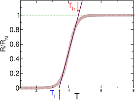
Figure 1: Sketch of the typical resistance curve for a superconducting interface (circles). The width of the transition can be estimated as $\Delta T_{c}/T_{c}\simeq(T_{h}-T_{l})/T_{l}$. Notice the persistance of a pronounced tail also below $T_{l}$. By closer inspection of the data in Ref. triscone, , one can see that for negative applied voltages $\lesssim-80$ V such a tail saturates to a low but finite resistance value.

Inspecting Table I one can easily see that the typical width of the superconducting transition in metal-oxide interfaces is substantially larger than the width of standard disordered films, that attain values comparable to those reported for the interfaces only at extremely large disorder concentration, where also the critical temperature is almost driven to zero. The observed temperature dependence of the sheet resistance in superconducting interfaces shows instead two characteristic features not reported in disordered films: (i) the transition width becomes large for relatively small variations of the critical temperature (compare the case $V=-40$ V and $V=-60$ V in Table I); (ii) an extended tail is observed below $T_{l}$ in a sample with an applied bias $V\lesssim-80V$, with the resistance saturating to a low but still finite value.triscone These two features call for a specific analysis to see whether in heterostructures these large transition widths and persisting tails arise from mesoscopic inhomogeneities.

Ref.	Sample	$T_{h}$ (K)	$T_{l}$ (K)	$\Delta T/T_{c}$
[triscone, ]	V=180 V	0.347	0.263	0.32
	V=100 V	0.338	0.260	0.3
	V=0 V	0.306	0.2	0.53
	V=-40 V	0.26	0.138	0.88
	V=-60 V	0.235	0.100	1.35
[sacepe1, ]	TiN1	1.71	1.34	0.28
	TiN2	1.34	1	0.34
	TiN3	0.83	0.47	0.76
[mondal, ]	$k_{F}\ell=3.27$	8.27	8.50	0.03
	$k_{F}\ell=1.58$	2.36	4	0.69

Table 1: Estimate of the superconducting transition width in superconducting interfaces (Ref. triscone, ) and disordered films of conventional superconductors (Refs. sacepe1, for TiN and mondal, for NbN). The labels used to identify the samples are the same used in the corresponding publications. In the case of Ref. triscone, $V$ is the bias potential applied to the SrTiO₃ substrate to change the charge density at the interface.

It is worth noting that such broad transitions can hardly be ascribed to ordinary superconducting fluctuations. Indeed, considering the Aslamazov-LarkinAL contribution of superconducting fluctuations to the paraconductivity [see Eq. (5) below], one obtains that $\Delta T/T_{c}=R_{N}/R_{c}$, where $R_{N}$ is the normal-state sheet resistance (i.e., approximately the value right above the beginning of the downturn of $R_{\square}(T)$) and $R_{c}=16\hbar/e^{2}=65.6$ k$\Omega$. Since $R_{N}$ values for the interfaces are of order of 1 k$\Omega$ or even smaller, ordinary superconducting fluctuations would give $\Delta T/T_{c}\simeq 0.02$, i.e., at least one order of magnitude smaller than the one reported in Table I. This result has to be contrasted, for example, to other systems like high-temperature superconducting oxydes,vidal where the conclusion was reached instead that fluctuation effects are enough to account for the width and rounding effects around $T_{c}$, while mesoscopic inhomogeneities play a minor role.

The disordered mesoscopic model we have in mind consists of large metallic regions with randomly distributed critical temperatures that we map into a network of random resistors. Upon decreasing $T$ more and more regions (links) become superconducting until a percolation threshold is reached and the superconducting transition occurs. The model can be solved by means of the so-called effective medium theory (EMT),effectivemedium ; kirkpatrick that is often used as a valuable guide to investigate the effects of mesoscopic inhomogeneities. However, to establish the degree of reliability of EMT in the case of different disorder realizations, we will compare the EMT results with exact numerical solutions on finite clusters. In particular, owing to the “mean-field-like” character of EMT, it is important to establish to what extent this approach can reliably be used in cases where space correlations are sizable.

We notice that in our model the superconducting regions are assumed to be large enough to have a fully established local coherence and to make negligible the charging effects. As a consequence, neighboring superconducting resistances immediately establish a mutual phase coherence as soon as both have become superconducting. This clearly distinguishes our framework from the case of granular superconductors, where the grains have usually nanoscopic sizes of the order of the coherence length of the pure system. Moreover, the large size of a mesoscopic domain also allows to consider paraconductivity effects (both á la Aslamazov-LarkinAL and á la Halperin-NelsonHN ) to occur within each domain.

Our paper is structured as follows. In Sec. II we summarize some results of the EMT in the case of mixed normal-superconducting states. In Sec. III we describe our numerical approach, where we find an exact solution to a network of random resistors with different local resistances and/or critical temperatures. Sec. IV is devoted to the analysis of different effects ($T_{c}$ distribution, inclusion of correlation between local $T_{c}$ and local resistance, gaussian or Berezinski-Kosterlitz-Thouless paraconductivity fluctuations) in the absence of space correlations. This last limitation is overcome in Sect. V, where different realizations of space correlations are considered. Our concluding remarks are reported in Sec. VI.

II Effective medium theory

The effective medium resistivity $\rho_{em}$ of a random resistor network, in which the value $\rho_{i}$ of the resistivity of a resistor on a bond of the network occurs with a frequency $w_{i}$, obeys the equationeffectivemedium ; kirkpatrick

$$\mathcal{F}(\rho_{em})\equiv\sum_{i}w_{i}\frac{\rho_{em}-\rho_{i}}{\rho_{em}+\alpha\rho_{i}}=0,$$ (1)

where the sum is carried over all the possible values of $\rho_{i}$, $\sum_{i}w_{i}=1$, and the parameter $\alpha$ is related to the connectivity of the network. For a cubic network in $D$ spatial dimensions, $\alpha=D-1$. Eq. (1) can be recast in the self-consistent form

$$\rho_{em}=\sum_{i}\frac{w_{i}\rho_{i}}{\rho_{em}+\alpha\rho_{i}}\left[\sum_{i}\frac{w_{i}}{\rho_{em}+\alpha\rho_{i}}\right]^{-1}\equiv\Phi(\rho_{em}),$$ (2)

with $\rho_{P}\leq\Phi(\rho_{em})\leq\rho_{S}$, $\rho_{P}\equiv[\sum_{i}w_{i}/\rho_{i}]^{-1}$, $\rho_{S}\equiv\sum_{i}{w_{i}\rho_{i}}$, and $\Phi^{\prime}(\rho_{em})\geq 0$. It is therefore evident that the function $\Phi(\rho_{em})$ interpolates between the parallel $\rho_{P}$ and the series $\rho_{S}$ of the resistors. Since in Eq. (1) $-1/\alpha\leq\mathcal{F}(\rho_{em})\leq 1$, and $\mathcal{F}^{\prime}(\rho_{em})>0$, Eq. (1) has a unique solution, which can be efficiently found, e.g., by bisection, within the interval $[\rho_{min},\rho_{MAX}]$, where $\rho_{min}$ and $\rho_{MAX}$ are, respectively, the smallest and largest possible values of the resistivity. Indeed, from Eq. (2), it is evident that $\rho_{min}\leq\rho_{P}\leq\rho_{em}\leq\rho_{S}\leq\rho_{MAX}$. We specialize the EMT to the case in which the random resistor network undergoes a metal-superconductor transition, by varying some control parameter, e.g., the temperature $T$, on which the resistivities $\rho_{i}$ depend. Lowering the temperature on the metallic side, an increasing number of resistors become superconducting and $\rho_{em}$ decreases. Near the transition $\rho_{em}\to 0^{+}$, and Eq. (1) can be linearized asnotaem

$$\left[\frac{1+\alpha}{\alpha}\sum_{\rho_{i}>0}\frac{w_{i}}{\rho_{i}}\right]\rho_{em}=1-(1+\alpha)\sum_{\rho_{i}=0}w_{i},$$

whence it is evident that the transition occurs when the total weight of the superconducting resistors, $w_{s}\equiv\sum_{\rho_{i}=0}w_{i}$, equals $1/(1+\alpha)$. On a square lattice $\alpha=1$ and we find that the EMT correctly reproduces the percolation threshold $w_{s}=1/2$ in two dimensions.

To gain further insight into the physics of the metal-superconductor transition within the EMT, let us initially assume that the resistivity on a bond of the random resistor network may take only two constant values, $0$ and $\rho_{0}>0$, and that the network is characterized by a distribution of $T_{c}$’s $\mathcal{W}(T_{c})$ of the individual resistors, with $\int_{-\infty}^{+\infty}dT_{c}\,\mathcal{W}(T_{c})=1$. Henceforth, to simplify the notation, we adopt a continuous description of the statistical distributions. Each resistor has a resistivity $\rho_{0}$ at high temperature and its resistivity vanishes as soon as the temperature $T$ is lowered below its critical temperature $T_{c}$, i.e., the resistivity of a bond is taken as $\rho=\rho_{0}\theta(T-T_{c})$, where $\rho_{0}$ is the same for all bonds and $T_{c}$ is a random variable. The distribution of resistivity in the system is therefore $w(\rho)=w_{s}(T)\delta(\rho)+[1-w_{s}(T)]\delta(\rho-\rho_{0})$, where $w_{s}(T)\equiv\int_{T}^{+\infty}dT_{c}\,\mathcal{W}(T_{c})$ is the statistical weight of the superconducting resistors at a temperature $T$, i.e., the frequency of occurrence of resistors with $T_{c}>T$. In such a case, Eq. (1) may be readily solved, to yieldkirkpatrick

$$\rho_{em}(T)=(1+\alpha)\rho_{0}\int_{T_{c}^{\alpha}}^{T}dT_{c}\,\mathcal{W}(T_{c})$$ (3)

for $T\geq T_{c}^{\alpha}$, and $\rho_{em}(T)=0$ for $T<T_{c}^{\alpha}$, where $T_{c}^{\alpha}$ is the critical temperature of the effective medium, which is defined by the equation

$$w_{s}(T_{c}^{\alpha})\equiv\int_{T_{c}^{\alpha}}^{+\infty}dT_{c}\,\mathcal{W}(T_{c})=\frac{1}{1+\alpha}.$$

Thus, for $T\to\infty$, $\rho_{em}\to\rho_{0}$, and $\rho_{em}(T_{c}^{\alpha})=0$. On passing, we note the interesting inversion formula $\mathcal{W}(T_{c})=\rho_{em}^{\prime}(T)|_{T=T_{c}}/[(1+\alpha)\rho_{0}]$, which holds for $T\geq T_{c}^{\alpha}$, and allows one to reconstruct the distribution of $T_{c}$’s for $T_{c}\geq T_{c}^{\alpha}$, from the behavior of the effective medium resistivity as a function of $T$. This relation holds provided that the normal-state resistivity $\rho_{0}$ does not depend on temperature. We apply the analytical solution (3) to a paradigmatic example which shall be used as a benchmark in the forthcoming analysis. Let us assume a distribution of $T_{c}$’s

$$\mathcal{W}(T_{c})=\frac{w_{1}}{\sqrt{2\pi}\sigma_{1}}{\mathrm{e}}^{-(T_{c}-T_{1})^{2}/2\sigma_{1}^{2}}+\frac{w_{2}}{\sqrt{2\pi}\sigma_{2}}{\mathrm{e}}^{-(T_{c}-T_{2})^{2}/2\sigma_{2}^{2}},$$

with $w_{1}+w_{2}=1$. This is a bimodal distribution of $T_{c}$’s, with two characteristic values, $T_{1}$ and $T_{2}$, and widths $\sigma_{1}$ and $\sigma_{2}$. As a limiting case, e.g., for $w_{2}=0$, a single Gaussian distribution is recovered. Specializing Eq. (3) to the present case, we find

$$\rho_{em}(T) = \frac{1+\alpha}{2}\rho_{0}$$ (4)

$$\times \left\{w_{1}\left[\mathrm{erf}\left(\frac{T-T_{1}}{\sqrt{2}\sigma_{1}}\right)-\mathrm{erf}\left(\frac{T_{c}^{\alpha}-T_{1}}{\sqrt{2}\sigma_{1}}\right)\right]\right.$$

$$+ \left.w_{2}\left[\mathrm{erf}\left(\frac{T-T_{2}}{\sqrt{2}\sigma_{2}}\right)-\mathrm{erf}\left(\frac{T_{c}^{\alpha}-T_{2}}{\sqrt{2}\sigma_{2}}\right)\right]\right\},$$

where $\mathrm{erf}(x)=\frac{2}{\sqrt{\pi}}\int_{0}^{x}dz\,\mathrm{e}^{-z^{2}}$. The equation that fixes $T_{c}^{\alpha}$ is

$$w_{1}\,\mathrm{erf}\left(\frac{T_{c}^{\alpha}-T_{1}}{\sqrt{2}\sigma_{1}}\right)+w_{2}\,\mathrm{erf}\left(\frac{T_{c}^{\alpha}-T_{2}}{\sqrt{2}\sigma_{2}}\right)=\frac{\alpha-1}{\alpha+1}.$$

As it will be clear below, such bimodal distribution turns out to reproduce quite well a large tail in the resistivity as $T_{c}^{\alpha}$ is approached, as in Fig. 1. Indeed, while for a single gaussian distribution both the EMT and the random-resistor network solution give a resistivity vanishing almost linearly at $T_{c}^{\alpha}$, when part of the system is not superconducting (i.e., $T_{2}$ vanishes) the transition occurs smoothly with a resistance vanishing with an upward curvature, in close resemblance with the experimental data in superconducting interfaces.triscone ; espci

III Exact solution of the random-resistor network

To have exact results and to test the reliability of the EMT, we solve numerically a system of resistors on a finite square lattice. Each link $(i,j)-(i+1,j)$ along $x$ or $(i,j)-(i,j+1)$ along $y$ of the lattice is characterized by a resistance which can vanish at a local critical superconducting temperature $T_{c}$. A given fixed voltage is applied at two opposite edges of the square $N\times N$ cluster, while the two other edges have open boundary conditions. Given a random distribution of resistivities and/or $T_{c}$’s on the links, the system adjusts the voltage at each node $(i,j)$ and the currents along each link by implementing Ohm’s law on the links and Kirchoff’s law for current conservation on the nodes. These laws provide a set of $3N^{2}-2N$ linear equations to be solved to determine the $N^{2}-2N$ voltages of the nodes (the voltages on two sides of the cluster are fixed) and the currents of the $2N^{2}$ links (the inside $N^{2}-2N$ links plus the $2N$ incoming and outgoing links). Of course the system could be reduced to a smaller number of equations by simply inserting by hand the expressions of the voltages or of the currents obtained by Ohm’s or Kirchoff’s laws. However, in order to get a more transparent mapping of currents and potentials on each link or node, we choose this straightforward representation. We proceed as follows. We extract from a given distribution (which can be spatially uncorrelated or correlated) a critical temperature on each link. Given $T_{c}$ on a link, the normal-state resistivity is determined. It can be taken as independent from $T_{c}$, or it can be larger for less metallic regions (i.e., those having a smaller $T_{c}$). The latter case is aimed to account for the effect of microscopic impurities on the critical temperature, and it will be discussed in Sec. IV-B within the context of the Finkelstein theory.finkelstein The resistors on the links can even display a temperature dependence to describe, e.g., the contribution of superconducting fluctuations to the reduction of $R$ upon approaching the local $T_{c}$. This case will be discussed in Sec. IV-A within the context of both Gaussian (Aslamazov-Larkin) or vortical (Berezinski-Kosterlitz-Thouless) superconducting fluctuations. In any case, at a given temperature a given random realization of $T_{c}$’s gives rise to a realization of normal-state resistivities. Then the set of linear Ohm’s and Kirchoff’s equations is numerically solved for a $N\times N$ clusters with $N$ ranging from 50 to 200. The total current $I$ flowing at one edge of the cluster is evaluated by summing the currents of the $N$ horizontal links (if the overall constant voltage difference $V$ is applied to the two equipotential sides at $x=1$ and $x=N$). The ratio $V/I$ determines the total resistance of the cluster at any given temperature for the specific random realization of $T_{c}$’s and of the related local resistances in each bond $R(T_{c},T)$. This exact numerical solution is then compared with the solution of the EMT.

IV Spatially uncorrelated distributions of critical temperatures

We start considering the case of spatially uncorrelated distributions of critical temperatures. As we mentioned above, we will consider a bimodal distribution as a possible realization of smoothly vanishing resistivity curves. The $T_{c}$ distribution is then formed by two gaussian peaks: the first one with weight $w_{1}$ is centered at a positive $\overline{T}_{c}=T_{1}$ representing metallic regions with finite superconducting temperatures, while the second Gaussian with a weight $w_{2}$ represents regions with non-superconducting character and it is located at negative $T_{c}$’s (the precise location of this second Gaussian is immaterial as long as its tail is negligible on the positive $T_{c}$ side). Typically we chose ${T}_{1}=1$ and $\sigma_{1}\approx 0.14-0.16$. The relative weights $w_{1}$ and $w_{2}=1-w_{1}$ of the two components of the bimodal distribution tunes the ratio between regions which can and cannot become superconducting. Of course the case of a simple Gaussian distribution of superconducting temperatures is recovered by choosing $w_{1}=1$. Fig. 2 reports the case where all the regions (both superconducting and non-superconducting) have the same normal-state resistivity $\rho_{0}=1$. As soon as $T$ decreases below the local $T_{c}$, the local resistor becomes superconducting and the local resistance is switched off. Starting from the purely Gaussian case $w_{1}=1$ (black solid lines) we progressively reduce the weight of the metallic-superconducting regions to $w_{1}=0.75$ (online red lines), $w_{1}=0.5$ (online green lines), and $w_{1}=0.4$ (online blue lines). This has two effects on the $\rho(T)$ curves: (i) the critical temperature decreases, and (ii) the superconducting transition width increases, and the $\rho(T)$ displays a finite tail which eventually saturates to a finite value when $w_{1}<0.5$. By defining the transition width as done in Fig. 1 one obtains the values reported in Table II. When $w_{1}=1$ the transition width can be estimated from Eq. (3), that gives the slope at the transition $\rho_{em}^{\prime}(T_{c})=2\rho_{0}{\mathcal{W}}(T_{c})=\sqrt{2/\pi}\rho_{0}/\sigma_{1}$, so that $\Delta T_{c}/T_{c}=\sqrt{\pi/2}(\sigma_{1}/T_{1})$. Since we are using a distribution having $\sigma_{1}/T_{1}=0.14$ we obtain $\Delta T_{c}/T_{c}\approx 0.18$, as reported in Table II. However, when $w_{1}$ decreases $\Delta T/T_{c}$ increases, and simultaneously $\rho(T)$ displays a positive upward curvature after the regime of linear decrease.

$w_{1}$	$\Delta T/T_{c}$
1	0.18
0.75	0.28
0.5	0.5
0.4	0.71

Table 2: Transition width for the bimodal distribution, according to the results shown in Fig. 2.

As far as the comparison between the EMT (the dashed lines) and the numerical exact results is concerned, as it is apparent in Fig. 2, they coincide at any value of $w_{1}$, except in a very small critical region around the transition. This is quite remarkable since it is commonly believed that EMT works well only for dilute systems or for binary alloys of chemical species with similar resistivity.effectivemedium Here the situation involves, instead, a binary alloy with finite ($=\rho_{0}$) and vanishing resistances at any relative concentration.

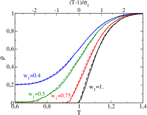
Figure 2: (Color online) Resistance curves for bimodal gaussian distribution of $T_{c}$’s. The solid lines are the exact results, the dashed ones report the EMT calculation. The upper scale is the deviation of $T$ from the average $\overline{T}_{c}$ in units of $\sigma_{1}$. The various colors refer to different weights of the two peaks of the bimodal distribution: black $w_{1}=1$; red $w_{1}=0.75$; green $w_{1}=0.5$; blue $w_{1}=0.4$. The upper peak of the bimodal distribution has an average $\overline{T_{c}}=1$ and variance $\sigma=0.14$.

We next explore the performance of EMT relaxing the assumption of constant normal-state $\rho_{0}$ for two cases of physical interest. In the first case a specific temperature dependence of the local resistances arises from paraconductive superconducting fluctuations inside each grain. In the second case quenched disorder induces a relation between the normal-state resistivities and the local critical temperature.

IV.1 Resistance with paraconductivity fluctuations

IV.1.1 Gaussian superconducting fluctuations

In the case of gaussian superconducting fluctuations the well-known theory by Aslamazov and LarkinAL introduces a power-law correction to the normal-state conductivity arising from Cooper-pair fluctuations. This increase of the conductivity diverges at $T_{c}$ with a prefactor which is universal in two dimensions even in the presence of disorder. Although other corrections to the conductivity become influential in the case of $s$-wave superconducting fluctuations, namely the Maky-Thompson contribution and the density of state corrections,varlamovlarkin in two dimensions the overall importance of the paraconductive corrections is well estimated by the universal Aslamazov-Larkin coefficient. This gives rather precise indications on the strength of the paraconductivity corrections and allows to avoid unrealistic assumptions on the role of paraconductive fluctuations in shaping the resistivity curves. Fig. 3 reports two cases in which the normal-state resistivity is lowered by paraconductivity effects according to the Aslamazov-Larkin theory of superconducting fluctuations. In this case

$$\rho_{0}(T)=\left(1+\frac{aT_{c}}{T-T_{c}}\right)^{-1}$$ (5)

when the local $T_{c}$ is lower than $T$, while it is zero as soon as $T$ becomes lower than $T_{c}$. Here $\rho_{0}(T)$ is the ratio of the resistivity to its normal-state value (so that $\rho_{0}(T)=1$ at high $T$), and within the ordinary AL theory the parameter $a$ is given in terms of the normal-state sheet resistance by $a=R_{N}/R_{c}$. Having in mind the experiments in the superconducting interfaces, where normal-state resistivity ranges bewteen $0.5$ and $2$ k$\Omega$,triscone ; espci ; sacepe1 ; sacepe2 ; sacepe3 ; mondal we use as an indicative value $a=0.05$. In Fig. 3(a) the critical temperatures have a Gaussian distribution, while Fig. 3(b) reports the case of a bimodal distribution with weight $w_{1}=0.5$ of the gaussian peak with finite average $T_{c}$. Again the EMT (dashed lines) reproduces well the exact numerical data (symbols) in both cases. We notice in passing that, although the paraconductivity correction diverges in each grain (i.e., in each resistor approaching its $T_{c}$), the effect on the whole system is vanishingly small around the global $T_{c}$. This can be understood thinking that around the global $T_{c}$ only a minor fraction of the resistors is still normal: for the whole system it makes little difference whether the very last few resistors of the percolating cluster have their resistance constant or lowered by AL fluctuations.

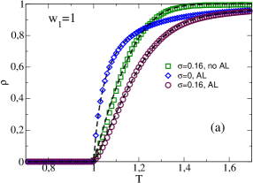
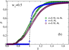
Figure 3: (Color online) Resistance curves in the presence of AL paraconductivity fluctuations and/or disorder. Symbols represent the exact results, the dashed lines report the EMT calculation. (a) Gaussian distribution of disorder. (Squares) Gaussian distribution of $T_{c}$’s with $\sigma=0.16$ and $\overline{T}_{c}=1$ and no AL fluctuations ($a=0$); (diamonds) resistance in the presence of AL fluctuations ($a=0.05$), but no disorder ($\sigma=0$); (circles) resistance in the presence of both AL fluctuations ($a=0.05$) and disorder ($\sigma=0.16$ and $\overline{T}_{c}=1$). (b) Same as in (a), but with a bimodal gaussian distribution of $T_{c}$’s with $w_{1}=0.5$.

In general we notice that the paraconductivity corrections do lower the slope of the resistivity curves thereby increasing the width of the global superconducting transition (compare squares and circles). However, it is also clear that assuming a realistic paraconductivity strength one cannot account for the experimentally observed transition widths without considering also a substantial effect of disorder (see diamonds). Resistivity slopes as small as the observed ones (see Table I) can only occur if the width is ruled by disorder (i.e., by the width of the $T_{c}$ distribution), while AL paraconductivity can at most provide a moderate increase of the width.

IV.1.2 Vortical superconducting fluctuations

Owing to the two-dimensional character of the superconducting films, we also consider the possibility that paraconductivity corrections might arise from vortical fluctuations.HN While the functional form of these corrections in terms of the coherence length $\xi$ is the same as for the Gaussian fluctuations, i.e., $\delta\sigma\propto\xi^{2}$, the prefactor is not universal and the temperature dependence reflects the exponential behavior of the coherence length in the Berezinski-Kosterlitz-Thouless (BKT) transition,HN ; benfatto09 i.e.,

$$\rho_{0}(T)=\left[1+A\sinh\left(\frac{b}{\sqrt{t}}\right)\right]^{-1}$$ (6)

where $t\equiv(T-T_{BKT})/T_{BKT}$ is the distance from the BKT transition temperature $T_{BKT}$, $A$ is a constant of order one, and the parameter $b$ is controlled by the distance bewteen the $T_{BKT}$ and the mean-field temperature $T_{c}^{0}$, above which Gaussian fluctuations are restored. As it has been discussed in detail in Ref. benfatto09, , $b=2\alpha\sqrt{t_{c}}$, where $t_{c}\equiv(T_{c}^{0}-T_{BKT})/T_{BKT}$ and $\alpha$ is a measure of the energy of the vortex core, expressed in units of the value it assumes within the standard $XY$-model approach to the BKT transition. Having in mind these definitions, we first explored the effect of local vortical paraconductivity fluctuations on the global superconducting transition using $t_{c}=0.1$, $\alpha=0.2$ (i.e., $b=0.126$), and $A=2$, which correspond to realistic parameter values, according to the estimates for thin disordered superconducting films in Ref. benfatto10, . The results are shown in Fig. 4 where, similarly to what found above for the Gaussian paraconductivity effects, we find that the most realistic estimate of the parameters produces only rather small corrections to the widths of the transition.

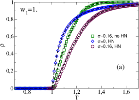
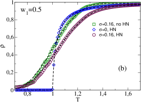
Figure 4: (Color online) Resistance curves in the presence of vortical paraconductivity fluctuations and/or disorder. The symbols represent the exact results, the dashed lines report the EMT calculation. (a) Gaussian distribution of disorder. (Squares) Gaussian distribution of $T_{c}$’s with $\sigma=0.16$ and no vortical fluctuations ($A=0$); (diamonds) resistance in the presence of vortical fluctuations [$t_{c}=0.1$, $\alpha=0.2$ ($b=0.126$), and $A=2$], but no disorder ($\sigma=0$); (circles) resistance in the presence both of vortical fluctuations [$t_{c}=0.1$, $\alpha=0.2$ ($b=0.126$), and $A=2$] and of disorder ($\sigma=0.16$). (b) Same as in (a), but with a bimodal gaussian distribution of $T_{c}$’s with $w_{1}=0.5$.

It is quite apparent from Figs. 3 and 4 that, for a realistic choice of parameters, the effects of AL fluctuations and vortical fluctuations are quite similar in the absence of disorder as well as in the presence of both a gaussian or a bimodal distribution of $T_{c}$’s.

Since in the literature the correct estimate of the parameters within the Halperin-Nelson formula (6) is often debated,benfatto09 we decided to explore further the limit of the BKT theory in reproducing correctly experimental data in superconducting interfaces. In particular, we considered also a set of parameters able to yield a larger transition width, regardless of their microscopic determination. In Fig. 5 we show the results for two set of Halperin-Nelson parameters and the related fit to data from an unbiased sample in Ref. triscone, . In panel (a) we report the results for a set (HN1) with $t_{c}=0.1$, $\alpha=0.4$ ($b=0.25$), and $A=2$, in the presence of a gaussian distribution of $T_{c}$’s ($w_{1}=1$) with $\sigma_{1}=0.035$ K and $\overline{T}_{c}=0.195$ K (black solid line) and for a similar set (HN1’) with $t_{c}=0.1$, $\alpha=0.4$ ($b=0.25$), and $A=1.8$, in the presence of a bimodal distribution of $T_{c}$’s ($w_{1}=0.5$) with $\sigma_{1}=0.025$ K and $\overline{T}_{c}=0.23$ K (blue dashed line). In panel (b), instead, we attempt to fit the same data with vortical fluctuations only (i.e., $\sigma=0$). Of course we need a quite more substantial amount of vortical fluctuations as given by a different (rather unrealisticnotaNbN ) parameter set (HN2), with $t_{c}=0.7$, $\alpha=0.8$ ($b=1.34$), and $A=0.71$.

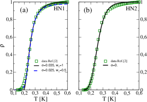
Figure 5: (Color online) (squares) Resistivity data of a LaAlO₃/SrTiO₃ sample at zero bias from Ref. triscone, . (a) (Black) Solid line, fit in the presence of both gaussian disorder ($w_{1}=1,\,\sigma_{1}=0.035$ K, and $\overline{T}_{c}=0.195$ K) and vortical fluctuations (HN1) with $t_{c}=0.1|$, $\alpha=0.4$ ($b=0.25$), and $A=2$. The (blue online) dashed line is for a similar parameter set (HN1’), with $t_{c}=0.1$, $\alpha=0.4$ ($b=0.25$), and $A=1.8$, and a bimodal distribution $w_{1}=0.5$, $\sigma_{1}=0.025$ K, and $\overline{T}_{c}=0.23$ K. (b) Squares, same as in (a); (black) solid line, fit in the presence of vortical fluctuations only (HN2) with $t_{c}=0.7$, $\alpha=0.8$ ($b=1.34$), $A=0.71$, and $T_{c}=0.157$ K.

It is apparent that vortical fluctuations alone can account for broad transitions [and also produce the tail characteristic of the LaAlO₃/SrTiO₃ (LAO/STO) or LaTiO₃/SrTiO₃ (LTO/STO) interfaces]. However, the parameters needed to produce the fit (which, by the way is quite poor in reproducing the high-temperature downward curvature) can hardly be justified on microscopic grounds. On the other hand, a moderate amount of disorder (notice that $T_{c}\approx 0.2$ K is in physical units here and therefore $\sigma_{1}\approx 0.03$ K is comparable with the values $\sigma_{1}/T_{c}\approx 0.15$ of the figures, having normalized $\overline{T}_{c}=1$) allows quite reasonable fits using a far more standard set of Halperin-Nelson parameters [see Fig. 5(a)]. We find also in this case that the overall width of the transition can be captured by the gaussian distribution of $T_{c}$’s (with a moderate contribution of superconducting fluctuations), but to reproduce the low-temperature tail one needs a bimodal distribution.

IV.2 Resistance with quenched disorder (Finkelstein’s theory)

Another physically interesting case occurs when quenched impurities affect the critical temperature of the grains. In Ref. finkelstein, a connection was established between disorder and the critical temperature in two-dimensional samples by deriving a relation between the resistance and the critical temperature in the presence of both disorder and Coulomb repulsion. Here, assuming that each grain is large enough to make the theory of Ref. finkelstein, applicable, we extract randomly (from a Gaussian distribution) the local critical temperatures of the resistors and we consequently assign the local resistivity. In practice we numerically invert the relation

$$\frac{T_{c}}{T_{c}^{0}}=e^{-\frac{1}{\gamma}}\left(\frac{\gamma-t/4+\sqrt{t/2}}{\gamma-t/4-\sqrt{t/2}}\right)^{\frac{1}{\sqrt{2t}}}$$ (7)

where, following the notation of Ref. finkelstein, , $T_{c}^{0}$ is the critical temperature of the clean system, $t\equiv R_{N}/R_{c}^{\prime}$, $\gamma\equiv 1/ln(T_{c}^{0}\tau)$, $\tau$ is the elastic scattering time, and the resistance $R_{c}^{\prime}\equiv 2\pi^{2}\hbar/e^{2}=81.1$ K$\Omega$. For the sake of concreteness, in our calculation we use $\gamma\approx-0.11$, obtained choosing $T_{c}^{0}=230$ mK as the superconducting temperature for the clean system and $\tau=5\times 10^{-7}$ mK^-1 for the value of the elastic scattering time. These values have been chosen to reproduce the correct orders of magnitude of experiments in LTO/STO samples.jerome The resulting $T_{c}$ vs. The $R_{N}$ curve is reported in the inset of Fig. 6. The results reported in Fig. 6 again display a quite good agreement between the exact numerical calculations and the EMT calculations (the barely visible dashed lines).

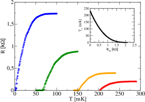
Figure 6: (Color online) Resistance for systems with gaussian distribution of local $T_{c}$’s centered at different average $T_{c}$’s and related local resistances from Eq. (7) with $R_{c}=81.1$ K$\Omega$, $T_{c}^{0}=230$ mK, and $\tau=5\times 10^{-7}$ mK^-1 (the inset reports the $T_{c}$ vs. $\rho$ curve corresponding to Eq. 7). The variance of the gaussian distribution is always $\sigma=30$ mK. Symbols refer to exact calculations while dashed lines report the EMT curves. The gaussian distributions are centered at $\overline{T}_{c}=0$ mK (blue circles and line), $\overline{T}_{c}=70$ mK (green squares and line), $\overline{T}_{c}=150$ mK (orange diamonds and line), and $\overline{T}_{c}=200$ mK, (red triangles and line).

We notice here that the progressive increase of the resistivity upon considering more disordered systems with lower $T_{c}$’s is associated with an increasing slope of the resistivity curves near $T_{c}$. By rescaling all the curves to let them assume the same high-temperature value $\rho_{0}(T\gg T_{c})=1$, the various curves are found to acquire quite similar slopes. This intriguing feature of our data is present in the case of LTO/STO interfaces, where, however, tails at $T\simeq T_{c}$ are also found, which are missing in our calculations of Fig. 6, carried out with a single gaussian distribution of local $T_{c}$’s.

V Spatially correlated distributions of critical temperatures

In all above cases the distribution of $T_{c}$’s and the consequent distribution of the resistances were spatially uncorrelated. This generically allows for a remarkably good performance of the EMT. Here, instead, we challenge EMT in the case of various space correlations.

V.1 Short-range averaged critical temperatures

In order to investigate the effects of short-range space correlations, we implement a short-range averaging procedure of the critical temperatures. As a first step, we extract the local $T_{c}$’s of the bonds on our cluster from a given gaussian distribution. Then, the value of $T_{c}$ on each bond is averaged with the values on the six nearest neighbor bonds. Of course, this yields gaussian distributed $T_{c}$’s with a variance reduced by a factor $\sqrt{7}$ and, at the same time, creates space correlations on distances of the order of two lattice spacings. This short-range correlation can be extended by iterating the averaging procedure: the once-averaged $T_{c}$’s can be averaged again with the six nearest neighbors, leading to space correlations up to four lattice spacings. The results we display below are always obtained with a two-step averaging protocol. Calculations with one- or three-step averaging procedures yield similar results. Fig. 7 reports with the solid black dots a calculation obtained starting from a Gaussian distribution with variance $\sigma=0.33$, centered at $\overline{T_{c}}=1$. The corresponding result for a EMT calculation is given by the black dashed line. Since EMT completely ignores the space correlations, the results are the same as those obtained with the starting uncorrelated set of random $T_{c}$’s, but for a trivial rescaling of the variance. Here, we numerically find that the variance entering the EMT expression [cf. Eq. (4)] with $w_{2}=0$ is $\sigma_{1}=0.09$. Clearly the averaging procedure spatially correlates the high-$T_{c}$ regions, which form short-range clusters. The inset in Fig. 7 displays a $100\times 100$ cluster in which the black regions correspond to regions where the local $T_{c}$ is larger than the average value $\overline{T_{c}}=1$. This lowers the exact resistance curve with respect to the EMT one, since the superconducting cluster is formed by objects with an effectively higher connectivity. Of course, this is true only far from percolation, because on a large scale it is instead immaterial whether the percolating objects are the single bonds or these small short-range clusters. Moreover, it is clear that the averaging procedure does not break the symmetry between high-$T_{c}$ and low-$T_{c}$ bonds (even if the variance is made smaller). Therefore, the percolation threshold stays the same and it is reached in two dimension when half of the bonds are superconducting. As a consequence, the curve of the exact calculation follows at high temperature the behavior of the EMT with a higher connectivity [this is represented by the (red online) dot-dashed line obtained from Eq. (4), with an effective connectivity numerically estimated to be $\alpha\approx 1.6$]. On the other hand, by lowering the temperature, the resistance is dominated by percolation effects, and a change of curvature occurs in $\rho(T)$, which vanishes at $T=1$, corresponding to a concentration 1/2 of superconducting bonds. This effect clearly introduces a “tailish” character in the low-$T$ part of the resistivity, which, however, is not large enough to reproduce quantitatively the data in LAO/STO and LTO/STO interfaces.

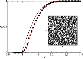
Figure 7: (Color online) Resistance of a short-range correlated random resistor network with $\overline{T}_{c}=1$ and a starting $\sigma=0.33$. The solids dots are the exact results, while the dashed line is obtained from numerical evaluation of the EMT, Eq. 1, with $\alpha=1$. The red dot-dashed line is instead obtained from Eq. 4, with $w_{1}=1$, $w_{2}=0$, $\alpha=1.6$, $T_{1}=0.997$, and $\sigma_{1}=0.09$.

V.2 Patches

Besides averaging the $T_{c}$’s over the first neighbors, we also introduce space correlations by simulating the occurrence of patches, where the $T_{c}$’s are similar in a region of given size. We first select a set of sites randomly distributed in our $N\times N$ cluster. Around each of these “seed” sites we define a patch of a given radius $r$. Then, we extract the critical temperatures inside the patches from a given gaussian distribution centered at a higher value of $\overline{T_{c}}$, while the bonds outside the patches have vanishing ${T}_{c}$. In this way, we aim to simulate a bimodal distribution with spatial correlation over a range $r$ typical of a sample where different extended regions have a more or less marked superconducting character.

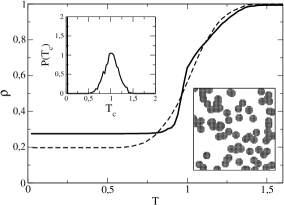
Figure 8: Resistance curves for a $100\times 100$ system with patchy structure (see lower inset). Each of the 80 patches (of radius $r=5$ lattice units) has a uniform local $T_{c}$ extracted from a Gaussian distribution with $\overline{T}_{c}=1$ and $\sigma=0.16$. The underlying matrix has local $T_{c}$’s extracted from a similar Gaussian centered at $\overline{T}_{c}=-100.$ (negative $T_{c}$’s are cumulated in $T_{c}=0$). The solid line is the exact result, while the dashed line is the EMT calculation. Upper inset: Total distribution of $T_{c}$’s.

The lower inset of Fig. 8 represents the case in which 80 patches with $r=5$ are introduced in a $100\times 100$ cluster. The main panel of Fig. 8 reports the related resistances both from exact (solid line) and EMT (dashed line) calculations. In both cases the system displays an initial rapid decrease of $\rho$, which then saturates at finite values upon decreasing $T$. While the EMT and exact data are quite similar at high temperatures, the low-$T$ saturation values are different. In particular the prediction of EMT is smaller than the exact result. Indeed, the exact solution is more resistive because the superconducting bonds are grouped into patches thereby leaving more extended surrounding regions, which are resistive. As a limiting case, one could imagine to form a single patch with weight 1/2 located inside the square cluster. Since one would have 1/2 of the bonds superconducting, EMT would predict the overall system to become superconducting. On the other hand, this single big patch being completely surrounded by a resistive region, the exact calculation would give a finite resistance for the system. This indicates that this realization of patches naturally results in higher resistances in the exact calculation, where the space correlation effects play a role, with respect to the EMT, where only the overall weight of superconducting bonds matters. In the present model, the size of superconducting regions can be increased either by increasing the number of patch centers (the “seeds”) and/or by increasing the radius of the patches $r$. Fig. 9 reproduces a case with 180 patches with $r=5$ in a $100\times 100$ cluster. Clearly (see lower inset), there is a large majority of highly superconducting sites, and the EMT predicts that the whole system becomes superconducting at $T_{c}=0.91$ (black dashed line in the main panel). Remarkably, this prediction reproduces well the exact solution given by the black solid line. However, close inspection of the lower inset shows that the superconducting character of the exact solution is only due to a small overlap of the patches in the central region of the cluster. If this small superconducting region were absent, the whole assembly of patches would not percolate and the system would display the finite resistance due to this small resistive region.

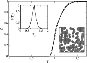
Figure 9: Same as in Fig. 8, but for a system with $180$ patches.

The above patchy structures have a random character, which makes it difficult to unambiguously establish the effective connectivity of the correlated regions. Therefore, we also investigated a toy model where the patches no longer form around random centers, but they form in a rather regular way. Specifically, we simply subdivided our $N\times N$ cluster into smaller $(N/d)\times(N/d)$ squares. This gives rise to a checkerboard support with $d\times d$ squares each having a given $T_{c}$ randomly extracted from a gaussian distribution. As a consequence, the critical temperatures of this coarse-grained system are still gaussian distributed but also display a strong space correlation, since they all coincide within each of the $d\times d$ square subclusters. We also notice in passing that to obtain a reasonably good Gaussian distribution quite large values of $N$ are required, because the statistical distribution of $T_{c}$’s is substantially degraded by extracting just one random $T_{c}$ inside each subcluster. We notice, however, that in this toy model each square subcluster is only connected to four other subclusters (but for a small effect in the corners). The exact calculation (not shown here) in this case agrees remarkably well with the prediction of the EMT. This demonstrates that connectivity plays a much more important role than the simple space correlation. Of course, whenever this latter influences the connectivity (like in the models of Secs. V A and V B), space correlation again becomes a main actor of the game.

V.3 Long-range spatially correlated distributions

To complete the analysis on the reliability of EMT in the presence of spatial correlations, we also investigate the behavior of the exact resistance and EMT when long range correlations are present. We empirically simulate this situation by adjusting the seeds of the random-number generator producing the distribution of random $T_{c}$’s, while visiting the $N\times N$ lattice sites, so that the $T_{c}$’s are highly correlated along lines. In particular, one can easily introduce long-range correlated patterns like the one reported in Fig. 10(a), where high values of $T_{c}$ along diagonals alternate with low values forming a stripe-like texture. In this case, the exact resistance displays rapid drops whenever the temperature reaches a value at which several neighboring bonds become simultaneously superconducting, substantially extending the size of the previously formed superconducting clusters [see the thin solid lines in Fig. 10(b)]. On the other hand, it then becomes difficult to build a fully percolating cluster and more or less sizable tails are generated. Lacking any information about the space structure of the random system, EMT fails in reproducing this situation. This is clearly visible comparing the two blue lines in Fig. 10(b), reporting the exact (solid) and EMT (dashed) results for the same specific random realization of Fig. 10(a).

The sharp drops occurring in the individual disordered realizations can however be smoothed by averaging over various realizations of the long-range correlated patterns (simulating, for instance, a system with differently oriented textures).

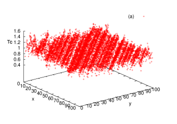
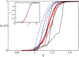
Figure 10: (Color online) (a) Example of a highly spatially correlated realization of random Gaussian distribution of $T_{c}$’s with $\overline{T}_{c}=1$ and $\sigma=0.1$. (b) Resistance curves for various realization of similar random spatially correlated $T_{c}$’s (thin solid black lines) and their average (thick solid red line). One of these specific curves has been drawn with a blue dot-dashed line together with its numerically calculated EMT (dashed line). Inset: The average resistance and a fit from Eq. (4) with $w_{1}=1$, $w_{2}=0$, $\alpha=0$ (corresponding to an effective dimensionality $D=1$), $T_{1}=1.155$, and $\sigma_{1}=0.075$.

The thick solid (red online) line in Fig. 10(b) is indeed obtained by averaging over the thin solid resistance curves obtained from seven different realizations with differently oriented and correlated diagonal stripes like the one reported in Fig. 10(a). As mentioned above, each of these realizations has a resistance quite different from that obtained with EMT. The (blue online) dashed line is the the EMT result obtained with the same gaussian distribution of local $T_{c}$’s used in Fig. 10 ($w_{1}=1$, $w_{2}=0$, $T_{1}=1$, and $\sigma_{1}=0.1$). We also fitted the average curve [see inset in Fig. 10(b)] by the analytic form in Eq. (4). This time the fit indicates an effective reduction of the connectivity, with $\alpha=0$ (i.e., $D=1$), $\overline{T}_{c}=T_{1}=1.15$, $\sigma_{1}=0.075$. While it is rather natural that some generic one-dimensional character arises from spatial correlations like in Fig. 10(a), the fact that the averaging procedure transforms the various quite different resistances of the individual realizations into a single nearly one-dimensional resistance curve is interesting.

VI Conclusions

In this paper we aimed to understand whether mesoscopic inhomogeneities could provide the physical mechanisms producing unusually broad superconducting transitions in various nearly two-dimensional systems, like the quasi-two-dimensional electron gases formed at the interfaces between SrTiO₃ and LaAlO₃ or LsTiO₃. Furthermore we wanted to get insights on the “tails” appearing in the resistance curves of LTO/STO and LAO/STO interfaces. By modeling the inhomogeneous system by a random resistor network, we systematically investigated various realizations of random resistors, which we solved both by an exact numerical approach and by a standard EMT approach. We started with the simple assumption of a random distribution of local $T_{c}$’s with global superconductivity occurring when superconducting regions (links) will eventually percolate by lowering the temperature. We then discussed various physical ingredients to account for the main experimental features of the superconducting transition at the interfaces. First of all, the transitions in these systems are anomalously broad and we clarified that this can hardly be attributed to standard gaussian or vortical (i.e., BKT-like) paraconductivity fluctuations. This is particularly evident for the AL paraconductivity, but it also holds for the Halperin-Nelson formula. Indeed, the set of parameters to be used to fit the experiments without disorder comes out to be rather unphysical. Therefore, superconducting fluctuation effects can contribute to, but cannot completely account for, the substantial width of the transition and for the small slopes of $R(T)$ around $T_{c}$. On the contrary, within our model the width of the transition mainly stems from the width of the distribution of $T_{c}$’s among the various superconducting mesoscopic regions. It turns out that a typical gaussian distribution of local $T_{c}$’s has the right downturn to mimic the experimental resistance curves, which display a moderate rounding above $T_{c}$ followed by a rather broad, nearly linear decrease when $T$ is lowered.

We also found in passing that the degree of reliability of EMT in solving different disorder realizations is high and standard EMT generically reproduces quite well the exact resistance curves, whenever the space correlations between the mesoscopic regions are negligible. This result is general, and is not limited to dilute systems or to mixtures of similar resistances. We rather find that EMT works well for mixtures of metallic (finite $R$) and superconducting (i.e., $R=0$) resistances, for any filling ratio, possibly including the effects of superconducting fluctuations. On the contrary, we find that increasing the space correlations leads to more substantial failures of the EMT.

An additional interesting and specific feature of the two-dimensional electron gas formed at the interface of the SrTiO₃ substrate is a more or less long tail in the low-$T$ part of the $R(T)$ resistance curves. These tails can even flatten to form a finite-$R$ plateau in cases where the system stays non superconducting despite a substantial decrease of $R(T)$ indicating the presence of a sizable superconducting fraction of the two-dimensional gas. We found that this feature is not easily reproduced and we only found few specific cases, where it could be reproduced within our model. In the case of non spatially correlated local $T_{c}$’s we found that a tail is only present when a bimodal distribution of $T_{c}$’s is assumed, with (or very near to) the specific $1/2-1/2$ distribution of the relative weight of the two distribution peaks. Since in the real systems the tails are observed over a broad range of fillings, magnetic fields, bias, it is hard to understand how these different conditions can all correspond to such specific $1/2-1/2$ constraint on the distribution of the mesoscopic local $T_{c}$’s. The $1/2-1/2$ condition can be rephrased by saying that at percolation, the whole set of superconducting domains randomly distributed in the two-dimensional system has to be exhausted.nota1D One possibility which deserves to be explored is that some microscopic mechanism acts to create some low-dimensional skeleton on which superconductivity takes place. Localization effects have already been proposed as a possible mechanism to generate a fractal substrate for superconductivityfeigelman and a glassy superconducting phase.ioffe ; feigelman10 If superconductivity occurred on this low-dimensional substrate, most if not all the bonds of the substrate have to be superconducting before the whole “skeleton” acts as a whole superconducting path.

A further mechanism to explore in order to reproduce tails in the resistance of the quasi-two-dimensional electron gas is provided by space correlations (indeed, the above scenario of fractal or glassy superconducting phase is a form of space correlation). When space correlations are short-ranged (see Sec. V A), we detect the presence of a short tail (see Fig. 7). One can expect that extending the strength and the range of these correlation could result into a strengthening of the tail feature. This expectation is confirmed by investigating space structures where more metallic domains cluster forming patchy textures embedded into less metallic matrices with very low or zero superconducting temperatures (see Figs. 8 and 9). In these cases again bimodal $T_{c}$ distributions are formed and again “tailish” resistances are obtained whenever the weight of the high-$T_{c}$ distribution peak approaches one half (or less when a plateau is obtained).

Finally, to reproduce tailish resistance curves, we explored the case of textured domains (forming, e.g., stripe-like paths) with long-range space correlations. If the real system is formed by a patchwork of randomly oriented stripe domains, one would obtain resistance curves with substantial tails (see Fig. 10). Indications of a spatially structured system hosting the two-dimensional electron gas have indeed been obtained from scanning tunneling microscopy experiments on LAO/STO samples,salluzzo suggesting that also this possibility is worth being further explored.

Acknowledgments. We are indebted with N. Bergeal, C. Di Castro, J. Lesueur, and J. Lorenzana, for interesting discussions and useful comments. We acknowledge financial support from MIUR Cofin 2007, Prot. 2007FW3MJX_003.

References

- (1) N. Reyren, S. Thiel, A. D. Caviglia, L. Fitting Kourkoutis, G. Hammerl, C. Richter, C. W. Schneider, T. Kopp, A.-S. R etschi, D. Jaccard, M. Gabay, D. A. Muller, J.-M. Triscone, and J. Mannhart, Science 317, 1196 (2007).
- (2) A. D. Caviglia, et al., Nature (London) 456, 624 (2008).
- (3) J. Biscaras, N. Bergeal, A. Kushwaha, T. Wolf, A. Rastogi, R. C. Budhani, and J. Lesueur, Nat. Commun., DOI: 10.1038, and arXiv:1002.3737
- (4) B. Sacépé, C. Chapelier, T. I. Baturina, V. M. Vinokur, M. R. Baklanov, and M. Sanquer, Phys. Rev. Lett. 101, 157006 (2008)
- (5) B. Sacépé, C. Chapelier, T. I. Baturina, V. M. Vinokur, M. R. Baklanov, and M. Sanquer, Nat. Commun. 1, 140 (2010).
- (6) B. Sacépé, T. Dubouchet, C. Chapelier, M. Sanquer, M. Ovadia, D. Shahar, M. Feigel’man, and L. Ioffe, Nat. Phys. 7, 239 (2011).
- (7) M. Mondal, A. Kamlapure, M. Chand, G. Saraswat, S. Kumar, J. Jesudasan, L. Benfatto, V. Tripathi, and P. Raychaudhuri, Phys. Rev. Lett. 106, 047001 (2011).
- (8) M. V. Feigel’man, L. B. Ioffe, V. E. Kravtsov, and E. Cuevas, Ann. Phys. 325, 1390 (2010).
- (9) A.M.Finkelstein, Sov. Phys. JETP Lett. 45, 46 (1987).
- (10) N. Bergeal and J. Lesueur, private communication.
- (11) M. Ma and P. A. Lee, Phys. Rev. B 32, 5658 (1985).
- (12) M. V. Feigel’man, L. B. Ioffe, V. E. Kravtsov, and E. A. Yuzbashyan, Phys. Rev. Lett. 98, 027001 (2007).
- (13) Y. Dubi, Y. Meir, and Y. Avishai, Nature 449, 876 (2007).
- (14) K. Bouadim, Y. L. Loh, M. Randeria, and N. Trivedi, arXiv:1011.3275.
- (15) L. B. Ioffe and M. Mézard, Phys. Rev. Lett. 105, 037001 (2010).
- (16) M. V. Feigel’man, L. B. Ioffe, and M. Mézard, arXiv:1006.5767.
- (17) L. G. Aslamazov and A. I. Larkin, Phys. Lett. A 26, 238 (1968); Sov. Phys. Solid State 10, 875 (1968).
- (18) J. Maza and F.Vidal, Phys. Rev. B43, 10560 (1991).
- (19) R. Landauer, in Electrical Transport and Optical Properties of Inhomogeneous Media, edited by J. C. Garland and D. B. Tanner (American Institute of Physics, New York, 1978), p. 2
- (20) S. Kirkpatrick, Rev. Mod. Phys. 45, 574 (1973).
- (21) This is true for . For , in a one-dimensional network, Eq. (1) has the exact analytical solution , whence it is evident that the network becomes superconducting only if all the resistors become superconducting.
- (22) See, e.g., A. Larkin and A. Varlamov, Theory of fluctuations in superconductors, (Clarendon Press, Oxford, 2005).
- (23) B. I. Halperin and D. R. Nelson, J. Low Temp. Phys. 36, 599 (1979).
- (24) L. Benfatto, C. Castellani, and T. Giamarchi, Phys. Rev. B 80, 214506 (2009).
- (25) A. Kamlapure, M. Mondal, M. Chand, A. Mishra, J. Jesudasan, V. Bagwe, L. Benfatto, V. Tripathi, and P. Raychaudhuri, Appl. Phys. Lett. 96, 072509 (2010).
- (26) For example, in Ref. benfatto10, the largest value obtained in a three-nanometer thick film of NbN is of order of .
- (27) A similar effect would occur in a one-dimensional system, where the superconducting transition takes place only when all the bonds (resistors) have become superconducting.
- (28) M. Salluzzo, private communication.