Thermodynamic and Structural Properties of the High Density Gaussian Core Model

Abstract

We numerically study thermodynamic and structural properties of the one-component Gaussian core model (GCM) at very high densities. The solid-fluid phase boundary is carefully determined. We find that the density dependence of both the freezing and melting temperatures obey the asymptotic relation, $\log T_{f}$, $\log T_{m}\propto-\rho^{2/3}$, where $\rho$ is the number density, which is consistent with Stillinger’s conjecture. Thermodynamic quantities such as the energy and pressure and the structural functions such as the static structure factor are also investigated in the fluid phase for a wide range of temperature above the phase boundary. We compare the numerical results with the prediction of the liquid theory with the random phase approximation (RPA). At high temperatures, the results are in almost perfect agreement with RPA for a wide range of density, as it has been already shown in the previous studies. In the low temperature regime close to the phase boundary line, although RPA fails to describe the structure factors and the radial distribution functions at the length scales of the interparticle distance, it successfully predicts their behaviors at shorter length scales. RPA also predicts thermodynamic quantities such as the energy, pressure, and the temperature at which the thermal expansion coefficient becomes negative, almost perfectly. Striking ability of RPA to predict thermodynamic quantities even at high densities and low temperatures is understood in terms of the decoupling of the length scales which dictate thermodynamic quantities from the interparticle distance which dominates the peak structures of the static structure factor due to the softness of the Gaussian core potential.

I Introduction

Complex fluids such as colloidal suspensions and emulsions are often regarded as macroscopic models of atomic or molecular systems. They are ideal benches to test liquid theories developed to describe thermodynamic, dynamic, and structural properties of atomic and molecular liquids Hansen and McDonald ((2006). It is not only because the size of constituent unit of complex fluids are much larger than atomic counterpart but also because their interparticle interactions can be tailor-made and tuned relatively easily. While the pair interactions of atomic systems are exclusively characterized by short-ranged and strong repulsions with weak and longer-ranged attractions, leading to the typical phase diagram demarcating gas, liquid, and crystalline phases Hansen and McDonald ((2006), those for the complex fluids are far more diverse. This diversity leads to very rich and often counter-intuitive macroscopic behaviors Likos ((2001). Amongst those interactions, the ultra-soft potential have attracted particular attention recently in the soft-condensed matter community Likos ((2006); Stillinger et al. ((1979, (1997); Lang et al. ((2000); Louis ((2000); Prestipino et al. ((2005); Mladek et al. ((2006); Mausbach et al. ((2006); Zachary et al. ((2008); Krekelberg et al. ((2009); Pond et al. ((2009); Krekelberg et al. ((2009); Shall and Egorov ((2010); Pond et al. ((2011); Marquest et al. ((1989); Likos et al. ((1998, (2001); Mladek et al. ((2006); Zhang et al. ((2010); Watzlawek et al. ((1999); Foffi et al. ((2003); Zaccarelli, Mayer, Asteriadi, Likos, Sciortino, Roovers, Iatrou, Hadjichristidis, Tartaglia, Lowen, and Vlassopoulos ((2005); Mayer, Zaccarelli, Stiakakis, Likos, Sciortino, Munam, Gauthier, Hadjichristidis, Iatrou, Tartaglia, Lowen, and Vlassopoulos ((2008); Pàmies et al. ((2009); Berthier and Witten ((2009); Berthier et al. ((2010). The ultra-soft potentials are isotropic repulsive potential characterized by weak and bounded repulsion at short distance and the mild repulsive tails whose steepness is much smaller than the typical atomic potential. These potentials are realized in many complex fluids such as star-polymers Watzlawek et al. ((1999); Foffi et al. ((2003); Zaccarelli, Mayer, Asteriadi, Likos, Sciortino, Roovers, Iatrou, Hadjichristidis, Tartaglia, Lowen, and Vlassopoulos ((2005); Mayer, Zaccarelli, Stiakakis, Likos, Sciortino, Munam, Gauthier, Hadjichristidis, Iatrou, Tartaglia, Lowen, and Vlassopoulos ((2008), dendrimers Likos ((2006); Gotze et al. ((2005); Mladek et al. ((2008), and the polymers in good solvent Louis ((2000); Krüger et al. ((1989); Dautenhahn et al. ((1994); Louis ((2000); Bolhuis ((2001). Thermodynamic phase diagrams of the ultra-soft particle systems have very distinct and exotic properties such as the re-melting from solid to fluid phase at high densities, the re-entrant peak at the intermediate densities Stillinger et al. ((1979); Lang et al. ((2000); Prestipino et al. ((2005); Zachary et al. ((2008); Zhang et al. ((2010); Watzlawek et al. ((1999); Pàmies et al. ((2009), negative thermal expansion coefficient Stillinger et al. ((1997); Mausbach et al. ((2006), and the cascades of the various crystalline phases at very high densities Watzlawek et al. ((1999); Pàmies et al. ((2009). The Gaussian core model (GCM) is one of the simplest examples of the ultra-soft potential systems. GCM consists of the point particles interacting with a Gaussian shaped repulsive potential;

$$v(r)=\epsilon\exp[-(r/\sigma)^{2}],$$ (1)

where $r$ is the interparticle separation, $\epsilon$ and $\sigma$ are the parameters which characterize the energy and length scales, respectively. GCM was first introduced by Stillinger Stillinger et al. ((1979) and has been studied by many groups Stillinger et al. ((1997); Lang et al. ((2000); Louis ((2000); Prestipino et al. ((2005); Mladek et al. ((2006); Mausbach et al. ((2006); Zachary et al. ((2008); Krekelberg et al. ((2009); Pond et al. ((2009); Krekelberg et al. ((2009); Shall and Egorov ((2010); Pond et al. ((2011). Despite of its simple form of the pair potential, GCM exhibits many typical thermodynamic behaviors of the ultra-soft particles. According to thermodynamic phase diagram obtained by numerical simulations Stillinger et al. ((1979); Prestipino et al. ((2005), GCM basically behaves like hard spheres at very low densities and temperatures; the crystalline structure in the solid phase is fcc and the freezing/melting temperatures sharply increase with density. However, as the density increases further, the freezing temperature reaches a maximal value and beyond this point it changes to a decreasing function of the density. This re-entrance takes place at $\rho\sigma^{3}\approx 0.25$, where $\rho$ is the number density. Concomitantly, the crystalline structure changes from fcc to bcc. Recently, thermodynamic and transport anomalies of the fluid phase in the vicinity of the reentrant peaks are investigated  Mausbach et al. ((2006); Krekelberg et al. ((2009); Pond et al. ((2009); Krekelberg et al. ((2009); Shall and Egorov ((2010); Pond et al. ((2011). Microscopic and structural properties such as the static structure factor in the fluid phase are also reported and documented Lang et al. ((2000); Louis ((2000); Mladek et al. ((2006); Zachary et al. ((2008). These studies revealed that, as the density increases beyond the reentrant peak but at a fixed temperature, thermodynamic and structural properties of GCM becomes more ideal-gas-like, signaled by the lowering of the peak of the structure factors and the better agreement with simple approximations such as the random phase approximation (RPA). Most of studies in the past, however, have focused on the densities not far from the reentrant peak or the relatively high temperatures. Less attention has been paid for the high density and low temperature regimes, especially in the vicinity of the solid-fluid phase boundary. Near the phase boundary line, the thermodynamic and structural properties are expected to be highly non-trivial even at the high density limit. Based on the duality argument of the ground state of GCM in the reciprocal space, Stillinger has conjectured that the freezing and melting temperatures, $T_{f}$ and $T_{m}$, are given by an asymptotic form;

$$\log T_{f},~{}\log T_{m}\propto-\rho^{2/3}$$ (2)

in the high density limit Stillinger et al. ((1979). However, this conjecture has not been confirmed numerically. Recently, we studied the nucleation and glassy dynamics of the one-component GCM in the supercooled state at the unprecedentedly high densities, $0.5\leq\rho\sigma^{3}\leq 2$ Ikeda and Miyazaki ((2011). It was found that the crystal nucleation rate decreases drastically as the density increases and concomitantly dynamics of the constituent particles becomes very sluggish. The density time correlation function exhibits typical behavior of the supercooled liquids near the glass transition point, such as the two-step and non-exponential structural relaxation. The relaxation time steeply increases as the temperature is lowered at a fixed density. Surprisingly, these are well described by the mode-coupling theory, implying that the high density and one-component GCM is more amenable to the mean-field picture of the glass transition than other typical glass formers. These observations call for more detailed analysis of the high density GCM at the low temperature regime. Especially, it is tempting to consider GCM in the high density limit as the ideal and clean model system to study the glass transition. Thermodynamic and structural characterization are prerequisites for dynamical study Ikeda and Miyazaki ((2011, unpublished) but the detailed study is lacking.

In this work, we numerically investigate thermodynamic and structural properties of the one-component GCM up to the density $\rho\sigma^{3}=2.4$. We determine the solid-fluid phase boundary and show that the Stillinger’s scaling, Eq. (2), holds at $\rho\sigma^{3}\gtrsim 1.2$. Thermodynamic and microscopic structural properties of GCM are also analyzed carefully over a wide range of temperature and density. The potential energy, pressure, thermal expansion coefficient, and the static structure factors are evaluated and compared with the prediction of the liquid state theory. Surprisingly good agreement with the random phase approximation (RPA) is found for thermodynamic quantities for a wide range of temperature, including the low temperature regimes where the same approximation poorly describes the static structure factor and radial distribution function. This counterintuitive observation can be attributed to the ultra-soft nature of GCM for which the microscopic structure near the first shell of the system decouples with the macroscopic properties.

This paper is organized as follows. In Section II, technical details of simulations and the method to compute the phase boundary are discussed. In Section III, we present simulation results for the phase diagram, thermodynamic quantities, and structural functions. We compare the simulation results in the fluid phase with RPA predictions in Section IV. We summarize and discuss the results in Sec. V.

II Simulation Method

II.1 MD and MC simulation

Thermodynamic state of GCM is fully characterized by the density $\rho$ and temperature $T$. In this work, we focus on the density and temperature range of $0.3<\rho^{\ast}<2.4$ and $10^{-6}<T^{\ast}<1$, where $\rho^{\ast}\equiv\rho\sigma^{3}$ and $T^{\ast}\equiv k_{\mbox{\scriptsize B}}T/\epsilon$. In order to analyze thermodynamic properties and determine the solid-fluid phase boundary, molecular dynamics (MD) simulations with Nosé thermostat are carried out under the periodic boundary conditions. To integrate the equations of motion, we use a reversible algorithm similar to the Velocity-Verlet method Frenkel and Smit ((2001) with time steps of $0.1\tau$, which is sufficiently short to preserve the Nosé Hamiltonian. Here $\tau=\sqrt{m\sigma^{2}/\epsilon}$ is the time unit, where $m$ is the mass of a particle. For evaluation of the free energy of the reference state (see below), Monte Carlo (MC) simulation is used. In a trial MC move, the maximum displacement of a particle is adjusted to keep the acceptance ratio about 50 %. In both simulations, the total number of particles is $N=3456$. This is twice the cube of an integer (in this case 12), a natural choice for the bcc crystal in a cubic simulation box. The cutoff length of the potential is taken as $5\sigma$. The pair potential at the cutoff length is $1.4\times 10^{-11}\epsilon$ which is much smaller than the typical kinetic energy at the lowest temperature studied in this work.

II.2 Evaluation of the free energy

The chemical potential as a function of the temperature and pressure, $\mu(T,P)$, is required in order to determine the phase boundary. We evaluate it using the free energy $f(T,\rho)$ and pressure $P(T,\rho)$.

We calculate the free energy using the thermodynamic integration method combined with the particle insertion method Widom ((1963) for the fluid phase and the Frenkel-Ladd method  Frenkel and Ladd ((1984) for the crystalline phase. This procedure is the same as the one employed by Prestipino et al. Prestipino et al. ((2005) for lower densities. The free energy of the system is the sum of the ideal $f_{id}$ and excess part $f_{ex}$. $f_{id}$ is given by $f_{id}(T,\rho)=k_{\mbox{\scriptsize B}}T(\log\Lambda^{3}\rho\sigma^{3}-1)$, where $\Lambda=\sqrt{2\pi\hbar^{2}/mk_{\mbox{\scriptsize B}}T}$ is the de Broglie thermal wave length. According to the thermodynamic integration scheme, $f_{ex}(T,\rho)$ can be evaluated by integrating over the energy and pressure from the reference state point $(T_{0},\rho_{0})$ to the target state point $(T,\rho)$ using the following equations.

$$\frac{f_{ex}(T,\rho_{0})}{T} =\frac{f_{ex}(T_{0},\rho_{0})}{T_{0}}+\int^{T}_{T_{0}}\!\!\!dT^{\prime}\ \frac{u(T^{\prime},\rho_{0})}{T^{\prime 2}},$$ (3)

$$\frac{f_{ex}(T,\rho)}{T} =\frac{f_{ex}(T,\rho_{0})}{T}+\int^{\rho}_{\rho_{0}}\!\!\!d\rho^{\prime}\!\!\ \left\{\frac{P(T,\rho^{\prime})}{\rho^{\prime 2}T}-\frac{1}{\rho^{\prime}}\right\},$$

where $u$ is the potential energy per particle. For the fluid phase, the reference free energy $f_{ex}(T_{0},\rho_{0})$ is calculated by the particle insertion method Frenkel and Smit ((2001); Widom ((1963) and the pressure is evaluated from the virial equation. In this method, the free energy is expressed in terms of the energy cost to insert one particle into the system as

$$\frac{f_{ex}(T_{0},\rho_{0})}{T_{0}}=-k_{\mbox{\scriptsize B}}\mbox{log}\left\langle{\exp\left(-\frac{E_{in}}{k_{\mbox{\scriptsize B}}T_{0}}\right)}\right\rangle-\frac{P_{0}}{\rho_{0}T_{0}}+1,$$ (4)

where $E_{in}$ is the interaction energy of an inserted particle with other particles in the system. The average should be taken over the ensemble of randomly inserted particles. For the crystalline phase, on the other hand, the reference free energy is computed using the Frenkel-Ladd method Frenkel and Smit ((2001); Frenkel and Ladd ((1984) which is a different kind of thermodynamic integration technique. In this method, we consider a hybrid Hamiltonian $\tilde{V}(\lambda)$, which interpolates between the Hamiltonian of the original system $V$ and that of the Einstein crystal $V_{ein}$ as $\tilde{V}(\lambda)=V+(1-\lambda)V_{ein}$, where $\lambda$ is the switching parameter. The free energy of the original system can be computed by the following equation, which is the integral over $\lambda$ of the Hamiltonian of the hybrid system evaluated from the simulation,

$$f_{ex}=f_{ex,ein}+\frac{1}{N}\int^{1}_{0}d\lambda\ \left\langle{V-V_{ein}}\right\rangle_{\lambda},$$ (5)

where $\left\langle{\cdots}\right\rangle_{\lambda}$ is the ensemble average under a hybrid Hamiltonian $\tilde{V}(\lambda)$ and $f_{ex,ein}$ is the excess part of the free energy of the Einstein crystal. We choose $(T_{0}^{\ast},\rho_{0}^{\ast})$ $=$(0.1, 0.01) and ($T_{0}^{\ast}$, $\rho_{0}^{\ast}$) $=$ (0.0794, 0.28) as the reference states for the fluid and crystalline phases, respectively. The ensemble averages in Eqs. (4) and (5) are evaluated using the MC simulations. The integration over $\lambda$ in Eq. (5) is calculated by slicing $\lambda$ to the grids of the width of 0.05 and evaluating the value of the integrand at each grid point from independent MC simulations. Likewise, the integral over the isothermal and isochoric pathways in Eq. (3) is computed by slicing the pathways into many grid points. The energy and pressure at each grid point are computed using the MD simulations. The free energy for both the fluid and crystalline phases are obtained by combining these data points and the reference free energy. In order to determine the solid-fluid phase boundary over the density range of $0.3<\rho^{\ast}<2.4$ with satisfactory accuracies, more than 800 grid points were necessary.

III Simulation results

III.1 Phase diagram

In his pioneering work, Stillinger has conjectured that the solid-fluid phase boundary is asymptotically given by Eq. (2) in the high density limit Stillinger et al. ((1979). This conjecture is based on analysis of the density dependence of the potential energy of various crystalline structures (bcc, fcc, etc) at $T=0$. According to his analysis, the potential energy is expressed as

$$u=-\frac{\epsilon}{2}+\frac{\pi^{3/2}\rho\sigma^{3}\epsilon}{2}\left\{1+A\exp(-K\rho^{2/3})+\cdots\right\},$$ (6)

where $A$ and $K$ are constants which depend on the crystalline structure. Stillinger argued that this density dependence remains qualitatively unchanged at finite temperatures. Since the ordered structure of the crystalline phase is responsible for the term $\exp(-K\rho^{2/3})$ in Eq. (6), the energy difference between the crystalline and fluid phase at the phase boundary should be also proportional to this term. This argument leads us to a conjecture that the melting/freezing temperature is proportional to this factor, which is Eq. (2). Here we verify this argument numerically.

Figure 1: The freezing ($T_{f}^{\ast}$) and melting ($T_{m}^{\ast}$) temperatures of GCM as a function of density (open up/down triangles). The result of Prestipino et al. is also plotted (filled circles with short-dashed line) Prestipino et al. ((2005). The long-dashed line is the threshold temperatures, $T_{th}$, above which RPA gives a reasonable description of the system (see Sec. IV). Open squares and dotted line indicate the temperature below which the thermal expansion coefficient becomes negative, $T_{\alpha}$, obtained from simulation and RPA, respectively. The short-dashed line at $\rho^{\ast}\approx 0.15$ demarcates the fcc (left) and bcc (right) crystalline phases.

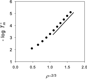
Figure 2: $-\log T^{\ast}_{m}$ versus $\rho^{\ast 2/3}$. The solid straight line is a guide for the eyes.

Figure 1 presents the phase diagram of GCM obtained from our simulation. Both the freezing and melting temperature $T_{f}^{\ast}$ and $T_{m}^{\ast}$ are shown in this figure, but their values are very close to each other and indistinguishable in the scale of the figure. As expected, the melting and freezing temperatures dramatically decrease as the density increases, down to $T^{\ast}\approx 10^{-6}$ at the highest density we studied. The phase boundary for $\rho^{\ast}\lesssim 0.7$ obtained by Prestipino et al. Prestipino et al. ((2005) is also plotted, in order to confirm that the present result perfectly matches with theirs for the density window where both results are available. The crystalline structure at high densities is bcc, as has been verified by the direct MD simulation of the nucleation Ikeda and Miyazaki ((2011, unpublished). In order to verify the scaling relation, Eq. (2), we plot the logarithm of the melting temperature as a function of $\rho^{2/3}$ in Fig. 2. One observes that the result rides on the scaling function at $\rho^{\ast}\gtrsim 1.2$.

III.2 Potential energy and pressure

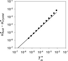
Figure 3: The potential energy difference between the crystalline and fluid phases against the melting temperatures with the fit by a straight line of the slope 1 (solid line).

The first order transition from the crystalline to fluid phase is accompanied with the discontinuous change in the structural order and the potential energy. We show the temperature dependence of the potential energy difference between the two phases $u^{\ast}_{fluid}(T_{f},\rho)-u^{\ast}_{crystal}(T_{f},\rho)$ as a function of $T_{m}$ in Fig. 3, where $u^{\ast}=u/\epsilon$ is the dimensionless potential energy. This figure shows that the energy difference is proportional to the melting temperature at the low temperatures/high densities, verifying the assumption which Stillinger has employed to conjecture Eq. (2). The entropy difference between the two phases can be estimated from this energy difference by $s_{fluid}(T_{f},\rho)-s_{crystal}(T_{f},\rho)=\left\{u_{fluid}(T_{f},\rho)-u_{crystal}(T_{f},\rho)\right\}/T_{f}$. From the result of Fig. 3, the entropy difference at the low temperature/high density limit can be estimated as

$$s_{fluid}(T_{f},\rho)-s_{crystal}(T_{f},\rho)\sim 0.45k_{\mbox{\scriptsize B}}.$$ (7)

This value should be compared with the results at lower densities in the earlier work; $0.81k_{\mbox{\scriptsize B}}$ at $\rho^{\ast}=0.4$ and $0.54k_{\mbox{\scriptsize B}}$ at $\rho^{\ast}=1.0$ Stillinger et al. ((1979).

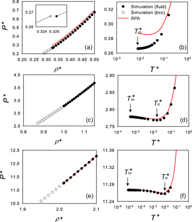
Figure 4: The equation of state of GCM. Filled and open circles are the results for fluid and crystalline (bcc) phases, respectively. Solid lines are the results from RPA (see Sec. IV). Left panels are $P$-$\rho$ plots at $T^{\ast}=$ $7.94\times 10^{-3}$ (a), $5.0\times 10^{-4}$ (c), and $7.9\times 10^{-6}$ (e). The inset in (a) is the closeup around the freezing transition density. Right panels are $P$-$T$ plots at $\rho^{\ast}=$ 0.33 (b), 0.99 (d), and 2.01 (f). $T^{\ast}_{m}$ and $T^{\ast}_{\alpha}$ (see text) are indicated by arrows.

Next we focus on the equation of state (EOS) of the high density GCM, i.e., the pressure as a function of the density and temperature. The dimensionless pressure $P^{\ast}\equiv P\sigma^{3}/\epsilon$ is plotted in Figure 4. In Figures 4 (a), (c), and (e), we plot the isothermal cut of EOS and the isochoric cut in Figures 4 (b), (d), and (f). The parameters $T^{\ast}$ and $\rho^{\ast}$ for each adjacent figures have been chosen so as for them to share the common freezing points; Fig. 4 (a) and (b) share the freezing point ($T_{f}^{\ast},\rho_{f}^{\ast})=(7.94\times 10^{-3},0.33$), (c) and (d) share ($T_{f}^{\ast},\rho_{f}^{\ast})=(5.0\times 10^{-4},1.00$), and (e) and (f) share ($T_{f}^{\ast},\rho_{f}^{\ast})=(7.9\times 10^{-6},2.01$). Figure 4 (a) shows that the melting of the bcc crystalline phase (white circles) to the fluid phase (filled circles) takes place at at $\rho^{\ast}\approx 0.33$. The inset shows the narrow coexistence region around the transition density, at which the pressure becomes constant. Similar behaviors of the first order transition are also observed in Figs. 4 (c) and (e) but at much higher densities.

Figure 4 (b) shows the equation of state at $\rho^{\ast}=0.33$ over the temperature range of $1.0\times 10^{-3}<T^{\ast}<1.0$. At this relatively low density, the pressure is a monotonically increasing function of the temperature, which is usual behavior of ordinary fluids. However, at higher densities, as shown in Fig. 4 (d) and (f), there exists the temperature regime in which the pressure becomes a decreasing function of temperature. In this regime, the thermal expansion coefficient $\alpha=V^{-1}(\partial V/\partial T)_{P}$ becomes negative. We determine the threshold temperature $T_{\alpha}$ at which $\alpha$ changes its sign by fitting the pressure by a smooth polynomial function and plot $T_{\alpha}$ in Fig. 1 (open squares). At low densities, $T_{\alpha}$ is located in the vicinity of the phase boundary. With increasing density, however, the difference between $T_{\alpha}$ and $T_{m}$ increases monotonically. Although the existence of the anomalous negative thermal expansion coefficient of GCM has been reported in the literatures Stillinger et al. ((1979, (1997), its high density behavior has not been explored. We shall discuss this result and its asymptotic behavior of $T_{\alpha}$ at high densities in the following section.

III.3 Static structure factor

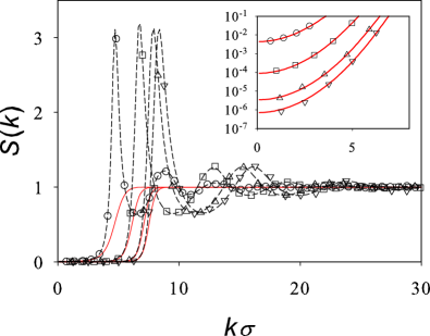
Figure 5: The static structure factors in the fluid phase at the freezing temperatures for $\rho^{\ast}=0.33$ ($\bigcirc$), $1.00$ ($\square$), $1.65$ ($\bigtriangleup$), and $2.01$ ($\bigtriangledown$). The dotted lines are the results obtained by the Fourier transformation of $g(r)$. The solid lines are the results of RPA (see Sec. IV). The inset is the semi-log plot of the main figure for $S(k)\leq 10^{-1}$ at low $k$’s.

In Figure 5, we show the static structure factors $S(k)$ in the fluid phase just above the freezing temperatures. $S(k)$ obtained from the Fourier transformation of the radial distribution function $g(r)$ is also shown. At all densities, $S(k)$’s exhibit sharp peaks similar to those of the ordinary simple fluids, such as the hard sphere and Lennard-Jones fluid, near the freezing temperatures. The peak position $k_{\max}$ shifts to high $k$’s as the density increases, $k_{\max}\propto\rho^{1/3}$, as one should expects at high densities. Note that, however, the height of the first peak is about 3.1 at all densities, which is slightly higher than the universal value 2.85 for the ordinary fluids which is known as Hansen-Verlet criterion Hansen and McDonald ((2006); Hansen and Verlet ((1969).

IV Random phase approximation analysis

IV.1 Random phase approximation

It is known that the thermodynamics and microscopic structure of the GCM fluid in high densities and temperatures are described by the random phase approximation (RPA) remarkably well Lang et al. ((2000); Louis ((2000). RPA is one of the approximation schemes of the liquid theory and a kind of the mean-field theory for the thermodynamics and structure of liquids Hansen and McDonald ((2006). In this section, we discuss how this approximation works at much lower temperatures.

It is convenient to divide thermodynamic quantities into uniform and fluctuation parts as follows. The potential energy can be represented as

$$u = -\frac{\epsilon}{2}+\frac{\pi^{3/2}\rho\sigma^{3}\epsilon}{2}+\Delta u,$$ (8)

where the first two terms are the uniform part and $\Delta u$ is the fluctuation part. $\Delta u$ can be expressed as

$$\Delta u = \frac{1}{4\pi^{2}}\int^{\infty}_{0}k^{2}\tilde{v}(k)S(k)\ dk,$$ (9)

where

$$\tilde{v}(k)=\pi^{3/2}\epsilon\sigma^{3}\exp(-k^{2}\sigma^{2}/4)$$ (10)

is the reciprocal expression of $v(r)$. Likewise, the pressure can be written, using the virial equation, as

$$P = k_{\mbox{\scriptsize B}}T\rho+\frac{\pi^{3/2}\rho^{2}\sigma^{3}\epsilon}{2}+\Delta P,$$ (11)

where the first two terms are the uniform part and the third is the fluctuation part which can be written as

$$\Delta P = \frac{\rho}{4\pi^{2}}\int^{\infty}_{0}\bigl{(}k^{2}-k^{4}\sigma^{2}/6\bigr{)}\tilde{v}(k)S(k)\ dk.$$ (12)

In RPA, the direct correlation function of the system is approximated as $c_{{\mbox{\scriptsize RPA}}}(r)=-\beta v(r)$, where $\beta=1/k_{\mbox{\scriptsize B}}T$. This approximation makes it possible to express various static quantities in simple and analytic forms. The static structure factor can be expressed as

$$S_{{\mbox{\scriptsize RPA}}}(k)=\frac{1}{1+\rho\beta\tilde{v}(k)}.$$ (13)

The fluctuation parts of the potential energy and pressure are expressed as Louis ((2000):

$$\Delta u_{{\mbox{\scriptsize RPA}}} =-\frac{\epsilon}{2\gamma}\mbox{Li}_{3/2}(-\gamma),$$ (14)

$$\Delta P_{{\mbox{\scriptsize RPA}}} =-\frac{\rho\epsilon}{2\gamma}\left\{\mbox{Li}_{3/2}(-\gamma)-\mbox{Li}_{5/2}(-\gamma)\right\},$$

where $\gamma=\pi^{3/2}\rho\sigma^{3}\epsilon/k_{\mbox{\scriptsize B}}T$ is a dimensionless coupling parameter and $\mbox{Li}_{\nu}(x)$ is the $\nu$-th polylogarithm function Louis ((2000); Mladek et al. ((2006). Furthermore, the radial distribution function at $r=0$ can be expressed analytically as

$$g_{{\mbox{\scriptsize RPA}}}(r=0)=1+\frac{1}{\pi^{3/2}\rho\sigma^{3}}\mbox{Li}_{3/2}(-\gamma).$$ (15)

The second term on the right hand side of this expression is negative for arbitrary densities and temperatures. At a very low temperature, the modulus of this term becomes larger than the first, leading to an unphysical negative $g(r=0)$. We refer to this temperature as the threshold temperature $T_{th}$. We plot $T_{th}$ in Fig. 1 (long-dashed line). At high densities, $T_{th}$ can be expressed analytically as

$$\frac{k_{\mbox{\scriptsize B}}T_{th}}{\epsilon}=\pi^{3/2}\rho\sigma^{3}\exp\left[-\Bigl{(}\frac{3\pi^{2}}{4}\rho\sigma^{3}\Bigr{)}^{2/3}\right],$$ (16)

which is obtained by the asymptotic expansion of polylogarithm function of Eq. (15) (see Appendix). Interestingly, the threshold temperature follows the same asymptotic scaling law $\log T_{th}\propto-\rho^{2/3}$ as the melting and freezing temperatures, Eq. (2). Note that this asymptotic expression is very accurate down to moderate densities $\rho^{\ast}\sim 1$.

IV.2 High temperature regime

Table 1: RPA results compared with simulation results for the fluctuation parts of the potential energy and pressure at the threshold temperatures for various densities.

$\rho$	0.10	0.33	1.00	3.00
${T_{th}}$	0.823	0.535	0.159	${0.689\times 10^{-2}}$
$\Delta u_{{\mbox{\scriptsize RPA}}}/\Delta u$	0.97	0.94	0.94	0.98
$\Delta P_{{\mbox{\scriptsize RPA}}}/\Delta P$	1.07	0.96	0.92	0.94

We first assess the validity of RPA at temperatures above $T_{th}$. Table 1 shows the ratio of RPA to simulation results of the fluctuation parts of the potential energy and pressure at $T=T_{th}$. The deviations are smaller than 10% and they monotonically become smaller as the temperature increases, implying the thermodynamic quantities are well-described by RPA even at $T_{th}$.

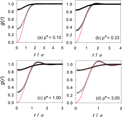
Figure 6: The radial distribution function in the high temperature regime for (a) $\rho^{\ast}=0.10$, (b) $0.33$, (c) $1.00$, and (d) $3.00$. Circles and lines are simulation and RPA results, respectively. Two results in each panel correspond to the results at the threshold temperature ($T^{*}=$ 0.823, 0.535, 0.159, and $0.689\times 10^{-2}$) and higher temperature at which $g_{{\mbox{\scriptsize RPA}}}(r=0)=0.83$ ($T^{*}=$ 5.76, 5.35, 4.30, and 2.29).

We also computed the radial distribution function $g(r)$. Fig. 6 shows $g(r)$ obtained from simulation (open circles) and RPA (solid lines) at $T=T_{th}$ and at much higher temperatures at which $g_{{\mbox{\scriptsize RPA}}}(r=0)=0.83$, for several densities. At high temperatures, agreement of simulation results with RPA is excellent in all densities and for all $r$’s. At $T=T_{th}$, however, RPA works poorly around $r=0$, as expected from Eq. (15). On the other hand, RPA’s results perfectly match with the simulation results at larger $r$’s including the first shell peaks. The reason why thermodynamic quantities are well described by RPA even at $T_{th}$ whereas agreement of $g(r)$ near $r=0$ is poor can be attributed to the fact that the short-range part of $g(r)$ does not contribute to both the potential energy and pressure, as we shall discuss in the following subsection.

IV.3 Low temperature regime

We move to temperatures below $T_{th}$ and discuss the validity of RPA in describing thermodynamic properties of GCM at high densities. In Fig. 5, the static structure factors obtained from RPA, $S_{{\mbox{\scriptsize RPA}}}(k)$, are shown in the solid lines. It is obvious that RPA cannot capture even the qualitative behaviors of $S(k)$; $S_{{\mbox{\scriptsize RPA}}}(k)$ remains flat at higher $k$’s and does not possess any prominent peak. However, as the main panel and inset of Fig. 5 shows, RPA correctly predicts the low $k$’s behavior up to just below the wavevector at which the first peaks are located. It is in stark contrast with ordinary simple atomic fluids for which RPA works poorly for the whole range of wavevectors . The excellent agreement implies that the mean-field character of the dense GCM still survives in the length scales slightly longer than the typical interparticle distance.

Next, we compare RPA with simulation results for thermodynamic quantities. We first look at the equation of state. In Fig. 4, the pressure obtained from RPA are plotted in solid lines. As shown in Fig. 4 (a) and (b), the deviation of the values of RPA from those of simulation is very large at $\rho^{\ast}=0.33$ and the discrepancies increase with decreasing temperature. RPA also predicts a fictitious negative thermal expansion coefficient at this density as shown in Fig. 4 (b). In high densities, however, agreement of RPA with simulation is excellent for all temperatures down to the freezing temperatures as shown in Fig. 4 (c)–(f). This is very surprising because the temperatures in these figures are far below $T_{th}$, where RPA fails to describe overall shapes of $S(k)$ as discussed in the previous subsection.

We also calculated $T_{\alpha,{\mbox{\scriptsize RPA}}}$ by solving $\partial P_{{\mbox{\scriptsize RPA}}}/\partial T=0$ and plotted in Fig. 1 (dotted line). Agreement of $T_{\alpha,{\mbox{\scriptsize RPA}}}$ with the simulation result is perfect except for the vicinity of the re-entrant melting region. The asymptotic expression of $T_{\alpha,{\mbox{\scriptsize RPA}}}$ which is valid at high densities can be written as (see Appendix)

$$\frac{k_{\mbox{\scriptsize B}}T_{\alpha,{\mbox{\scriptsize RPA}}}}{\epsilon}=\pi^{3/2}\rho\sigma^{3}\exp\ \left[-\left(\frac{{15}\pi^{2}}{4}\rho\sigma^{3}\right)^{2/5}-2\right].$$ (17)

This asymptotic expression works well down to $\rho^{\ast}\sim 1$ as in the case of $T_{th}$. Interestingly, the density exponent $2/5$ in this expression is smaller than $2/3$ for $T_{th}$ and $T_{m}$ (see Eqs. (2) and (16)). Due to this difference, $T_{\alpha}$ monotonically deviates from $T_{m}$ as the density increases and it eventually becomes larger than $T_{th}$ in the high density limit (not shown).

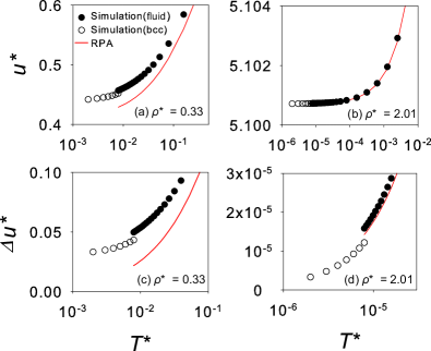
Figure 7: The temperature dependence of $u$ and $\Delta u$ at $\rho^{\ast}=0.33$ ((a) and (c)) and $\rho^{\ast}=2.01$ ((b) and (d)). Filled and open circles represent the simulation results for the fluid and crystalline (bcc) phase, respectively. Solid lines are the RPA results for the fluid phase.

We made similar comparison for the potential energy in Fig. 7. Fig. 7 (a) and (b) show the temperature dependence of the potential energy in the fluid phase (filed circles) and crystalline phase (open circles) at two densities. The uniform part of $u$ is temperature independent (see Eq. (8)), although it dominates the net values of $u$. In order to see the temperature dependence of $u$ more clearly, the fluctuation part $\Delta u$ are shown in Fig. 7 (c) and (d). One observes that agreement of the simulation results with RPA is far better at high densities; At $\rho^{\ast}=0.33$, RPA underestimates $\Delta u$ and discrepancy from the simulation data are larger than the energy gap between the fluid and crystalline phases. At the higher density $\rho^{\ast}=2.01$, the discrepancy is less 10% even at the freezing temperature.

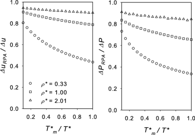
Figure 8: Temperature dependence of the ratio of RPA to simulation values of the fluctuation part of the potential energy (left) and the pressure (right) for $\rho^{\ast}=0.33$ ($\bigcirc$), $1.00$ ($\square$), and $2.01$ ($\bigtriangleup$). The range of temperatures in these figures is much lower than the corresponding $T_{th}$. ($T_{m}^{*}/T_{th}^{*}$ are $1.48\times 10^{-2}$, $3.14\times 10^{-3}$, and $2.55\times 10^{-4}$ for $\rho^{\ast}=0.33$, $1.00$, and $2.01$, respectively.)

In order to quantify the accuracy of RPA for both the potential energy and pressure, we plot the ratios of $\Delta u$ and $\Delta P$ of simulation to those of RPA in Fig. 8 against the inverse temperatures for several densities. The ratios decrease rapidly as the temperature decreases at the low density $\rho^{\ast}=0.33$, whereas, in the high density $\rho^{\ast}=2.01$, the ratios for both the potential energy and pressure remain to be more than 80% for the whole range of temperatures down to the melting temperature.

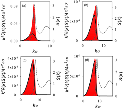
Figure 9: The integrand of Eq. (9) (shaded areas), the integrand where $S(k)$ is replaced with $S_{{\mbox{\scriptsize RPA}}}(k)$ (solid lines) and $S(k)$ (broken lines) for (a) $T^{\ast}=7.9\times 10^{-3}$ and $\rho^{\ast}=0.33$, (b) $T^{\ast}=5.0\times 10^{-4}$ and $\rho^{\ast}=1.00$, (c) $T^{\ast}=3.2\times 10^{-5}$ and $\rho^{\ast}=1.65$ and (d) $T^{\ast}=7.9\times 10^{-6}$ and $\rho^{\ast}=2.01$.

Given that RPA poorly describes even the qualitative behaviors of $S(k)$ and $g(r)$ at the high density and low temperature regimes, it is very surprising and counterintuitive that RPA is excellent at predicting quantitatively thermodynamic quantities $u$ and $P$. In order to rationalize this puzzling facts, we look again the integral expressions of the thermodynamic functions, Eq. (9) and (12). These expressions show that both $\Delta u$ and $\Delta P$ are expressed in terms of the integral of $S(k)$ multiplied with the pair potential over the wavevectors. In order to see which length scales dominate the integrand, we show the integrand of $\Delta u$ in Eq. (9) with simulated $S(k)$ in Fig. 9 (shaded area), along with those obtained using $S_{{\mbox{\scriptsize RPA}}}(k)$ (solid line). At the low density $\rho^{\ast}=0.33$, the integrand with simulated $S(k)$ is peaked at the peak position of $S(k)$ (broken line). This implies that $\Delta u$ at this density is dominated by the contribution at the interparticle distance, just like ordinary atomic fluids. The integrand obtained using RPA fails to account for this peak structure (solid line). However, with increasing density, the peak position of the integrand shifts to smaller wavevectors than the first peak position of $S(k)$. Concomitantly, agreement of the integrand obtained from simulation and RPA becomes better and better. This agreement originates from the fact that RPA can account excellently for the low wavevector behavior of the static structure factor as shown in Fig. 5. At very high densities, the particles start overlapping and the characteristic interparticle distance decouples with the length scales which dominate thermodynamic quantities of GCM. This is the reason why RPA remains the excellent approximation to predict thermodynamic quantities even far below the threshold temperatures.

V Conclusions

In this paper, we have presented a detailed analysis of thermodynamic and structural properties of the high density one-component GCM. Special emphasis has been put for static properties of the fluid phase. First, the solid-fluid phase boundary of the system is carefully evaluated up to the unprecedentedly high density $\rho^{\ast}=2.4$. Our result confirmed the scaling conjectured by Stillinger for the freezing and melting temperatures, $\log T_{f},~{}\log T_{m}\propto-\rho^{2/3}$, at $\rho^{\ast}\gtrsim 1.2$. The potential energy difference between the crystalline and fluid phases was shown to be linear in the freezing temperature and the entropy difference is almost constant at high densities, which verifies the assumption which Stillinger’s argument is based upon. The thermodynamic and structural properties of GCM in the fluid phase are analyzed in detail for a wide range of temperature and density. The potential energy $u$, the equation of state $P$, the static structure factor $S(k)$, and the radial distribution function $g(r)$ were evaluated by simulation. We compare the simulation results with the RPA results. In the high temperature regime, RPA provides almost perfect description for both thermodynamic quantities and the structural factor $S(k)$. RPA is rather poor at predicting $g(r)$ at $r\approx 0$. Threshold temperature $T_{th}$ below which RPA fails to describe $g(r=0)$ is relatively high. In the high density and low temperature regime, RPA fails to capture the peak structure of $S(k)$ even qualitatively, whereas it predicts correctly the low $k$’s behavior up to just below the wavevector at which the first peaks are located. Despite of poor performance of RPA at describing the structural properties, RPA successfully describes thermodynamic quantities such as the potential energy and pressure at high densities. Agreement of RPA with simulation results systematically improves as the density increases even near the phase boundary. The temperature below which the thermal expansion coefficient become negative is also accurately calculated from RPA. By scrutinizing the role of the microscopic structure of particles in the potential energy and pressure, we concluded that the surprising success of RPA is originated from the decoupling of the length scales which dictate the thermodynamic quantities and the interparticle distance. This decoupling is attributed to the mild and long-ranged repulsive tails of the pair potential of GCM. The fact that RPA is an excellent approximation even at the vicinity of the phase boundary, or even at the supercooled regime, at high densities, hints that the mean-field description is valid for the high density GCM and may play a crucial role to understand (glassy) dynamics let alone thermodynamic properties Ikeda and Miyazaki ((2011, unpublished).

Appendix A Derivation of Eqs. (16) and (17)

In this appendix, we derive the asymptotic expressions of $T_{th}$ and $T_{\alpha,{\mbox{\scriptsize RPA}}}$ at high densities by using the asymptotic expansion of the polylogarithm Wood ((1992)

$$\mbox{Li}_{\nu}(-x)=-\frac{(\log x)^{\nu}}{\Gamma(\nu+1)}+\mathcal{O}((-\log x)^{\nu-2}),$$ (18)

where $\Gamma(x)$ is the gamma function.

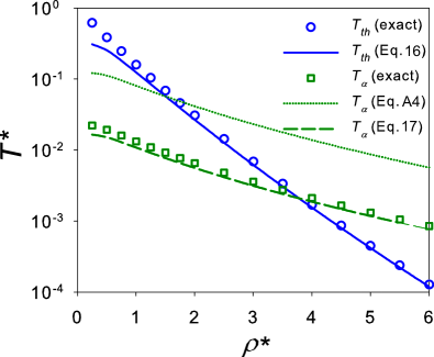
Figure 10: The validity of the asymptotic expressions for $T_{th}$ and $T_{\alpha,{\mbox{\scriptsize RPA}}}$. Open circles and solid line are RPA values and its asymptotic expression, Eq. (16), of $T_{th}$, respectively. Open squares, dotted line, and dashed line are RPA values and its two asymptotic expressions, Eqs. (21) and (17), of $T_{\alpha,{\mbox{\scriptsize RPA}}}$, respectively.

At $T=T_{th}$, Eqs. (15) and (18) lead to

$$\rho^{\ast}-\frac{4}{3\pi^{2}}\left(\log x_{th}\right)^{3/2}+\mathcal{O}\left(\left(\log x_{th}\right)^{-1/2}\right)=0,$$ (19)

where $x_{th}=\pi^{3/2}\rho^{\ast}/T_{th}^{\ast}$. When $\rho^{\ast}$ is sufficiently large, we can neglect the third term on the left hand side, leading to the asymptotic expression of $T_{th}$ of Eq. (16). Fig. 10 shows that this asymptotic expression is very accurate down to $\rho^{\ast}\sim 1$. Likewise, at $T=T_{\alpha,{\mbox{\scriptsize RPA}}}$, Eqs. (14) and (18) lead to

$$\rho^{\ast}-\frac{4}{15\pi^{2}}\left(\log x_{{\mbox{\scriptsize RPA}}}\right)^{5/2}+\frac{4}{3\pi^{2}}\left(\log x_{{\mbox{\scriptsize RPA}}}\right)^{3/2}$$ (20)

$$+\mathcal{O}\left(\left(\log x_{{\mbox{\scriptsize RPA}}}\right)^{1/2}\right)=0,$$

where $x_{{\mbox{\scriptsize RPA}}}=\pi^{3/2}\rho^{\ast}/T_{\alpha,{\mbox{\scriptsize RPA}}}^{\ast}$. If we neglect the third and fourth terms on the left hand side, we obtain

$$T_{\alpha,{\mbox{\scriptsize RPA}}}^{\ast}=\pi^{3/2}\rho^{\ast}\exp\left[-\left(\frac{15\pi^{2}\rho^{\ast}}{4}\right)^{2/5}\right].$$ (21)

However, Fig. 10 shows that this expression is not accurate even at very high densities. For sufficient accuracy, we have to keep the third term on the left hand side of Eq. (20). If we neglect only the forth term on the left hand side, Eq. (20) becomes

$$\frac{4}{15\pi^{2}}s^{5/2}-\rho^{\ast-2/5}\frac{4}{3\pi^{2}}s^{3/2}-1=0,$$ (22)

where $s=\rho^{\ast-2/5}\log(\pi^{3/2}\rho^{\ast}/T_{\alpha}^{\ast})$. Since the second term on the left hand side of this equation is small due to the factor $\rho^{\ast-2/5}$, we can expand the solution as $s=s_{0}+\rho^{\ast-2/5}s_{1}+\cdots$ and can solve the equation in each order of density. The first order solution including $s_{0}$ and $s_{1}$ is

$$s=\Bigl{(}\frac{15\pi^{2}}{4}\Bigr{)}^{2/5}+2\rho^{\ast-2/5},$$ (23)

which leads to the asymptotic expression of $T_{\alpha,{\mbox{\scriptsize RPA}}}$ of Eq. (17). Fig. 10 shows that this expression is very accurate down to $\rho^{\ast}\sim 1$.

References

- Hansen and McDonald ((2006) J. P. Hansen and I. R. McDonald, ”Theory of simple liquids” (Academic Press, 2006).
- Likos ((2001) C. N. Likos, Phys. Rep. 348, 267 (2001).
- Likos ((2006) C. N. Likos, Soft Matter 2, 478 (2006).
- Stillinger et al. ((1979) F. H. Stillinger, J. Chem. Phys. 65, 3968 (1976); F. H. Stillinger and T. A. Weber, ibid. 70, 4879 (1979); F. H. Stillinger, Phys. Rev. B 20, 299 (1979).
- Stillinger et al. ((1997) F. H. Stillinger and D. K. Stillinger, Physica A 244, 358 (1997).
- Lang et al. ((2000) A. Lang, C. N. Likos, M. Watzlawek, and H. Löwen, J. Phys.: Condens. Matter 12, 5087 (2000).
- Louis ((2000) A. A. Louis, P. G. Bolhuis, and J. P. Hansen, Phys. Rev. E 62, 7961 (2000).
- Prestipino et al. ((2005) S. Prestipino, F. Saija, and P. V. Giaquinta, Phys. Rev. E 71, 050102(R) (2005); S. Prestipino, F. Saija, and P. V. Giaquinta, J. Chem. Phys. 123, 144110 (2005).
- Mladek et al. ((2006) B. M. Mladek, G. Kahl and M. Neumann, J. Chem. Phys. 124, 064503 (2006).
- Mausbach et al. ((2006) P. Mausbach, and H. O. May, Fluid Phase Equilib. 249, 17 (2006).
- Zachary et al. ((2008) C. E. Zachary, F. H. Stillinger and S. Torquato, J. Chem. Phys. 128, 224505 (2008).
- Krekelberg et al. ((2009) W. P. Krekelberg, T. Kumar, J. Mittal, J. R. Errington, and T. M. Truskett, Phys. Rev. E 79, 031203 (2009).
- Pond et al. ((2009) M. J. Pond, W. P. Krekelberg, V. K. Shen, J. R. Errington, and T. M. Truskett, J. Chem. Phys. 131, 161101 (2009).
- Krekelberg et al. ((2009) W. P. Krekelberg, M. J. Pond, G. Goel, V. K. Shen, J. R. Errington, and T. M. Truskett, Phys. Rev. E 80, 061205 (2009).
- Shall and Egorov ((2010) L. A. Shall and S. A. Egorov, J. Chem. Phys. 132, 184504 (2010).
- Pond et al. ((2011) M. J. Pond, J. R. Errington, and T. M. Truskett, arXiv:1101.1982.
- Marquest et al. ((1989) C. Marquest and T. A. Witten, J. Phys. (Paris) 50, 1267 (1989).
- Likos et al. ((1998) C. N. Likos, M. Watzlawek, and H. Löwen, Phys. Rev. E 58, 3135 (1998).
- Likos et al. ((2001) C. N. Likos, A. Lang, M. Watzlawek and H. Löwen, Phys. Rev. E 63, 031206 (2001).
- Mladek et al. ((2006) B. Mladek, D. Gottwald, G. Kahl, N. Martin and C. N. Likos, Phys. Rev. Lett. 96, 045701 (2006).
- Zhang et al. ((2010) K. Zhang, P. Charbonneau, and B. M. Mladek, Phys. Rev. Lett. 105, 245701 (2010).
- Watzlawek et al. ((1999) M. Watzlawek, C. N. Likos, and H. Löwen, Phys. Rev. Lett. 82, 5289 (1999).
- Foffi et al. ((2003) G. Foffi, F. Sciortino, P. Tartaglia, E. Zaccarelli, F. Lo Verso, L. Reatto, K. A. Dawson, and C. N. Likos, Phys. Rev. Lett. 90, 238301 (2003).
- Zaccarelli, Mayer, Asteriadi, Likos, Sciortino, Roovers, Iatrou, Hadjichristidis, Tartaglia, Lowen, and Vlassopoulos ((2005) E. Zaccarelli, C. Mayer, A. Asteriadi, C. N. Likos, F. Sciortino, J. Roovers, H. Iatrou, N. Hadjichristidis, P. Tartaglia, H. Löwen, and D. Vlassopoulos, Phys. Rev. Lett. 95, 268301 (2005).
- Mayer, Zaccarelli, Stiakakis, Likos, Sciortino, Munam, Gauthier, Hadjichristidis, Iatrou, Tartaglia, Lowen, and Vlassopoulos ((2008) C. Mayer, E. Zaccarelli, E. Stiakakis, C. N. Likos, F. Sciortino, A. Munam, M. Gauthier, N. Hadjichristidis, H. Iatrou, P. Tartaglia, H. Löwen, and D. Vlassopoulos, Nat. Mater. 7, 780 (2008).
- Pàmies et al. ((2009) J. C. Pàmies, A. Cacciuto, and D. Frenkel, J. Chem. Phys. 131, 044514 (2009).
- Berthier and Witten ((2009) L. Berthier and T. A. Witten, Phys. Rev. E 80, 021502 (2009).
- Berthier et al. ((2010) L. Berthier, A. J. Moreno, and G. Szamel, Phys. Rev. E 82, 060501(R) (2010).
- Gotze et al. ((2005) I. O. Götze and C. N. Likos, J. Phys.: Cond. Matt. 17, S1777 (2005).
- Mladek et al. ((2008) B. M. Mladek, G. Kahl and C. N. Likos, Phys. Rev. Lett. 100, 028301 (2008).
- Krüger et al. ((1989) B. Krüger, L. Schäfer and A. Baumgärtner, J. Phys. (France) 50, 3191 (1989).
- Dautenhahn et al. ((1994) J. Dautenhahn and C. K. Hall, Macromolecules 27, 5399 (1994).
- Louis ((2000) A. A. Louis, P. G. Bolhuis, J. P. Hansen and E. J. Meijer, Phys. Rev. Lett. 85, 2522 (2000).
- Bolhuis ((2001) P. G. Bolhuis, A. A. Louis, J. P. Hansen and E. J. Meijer, J. Chem. Phys. 114, 4296 (2001).
- Ikeda and Miyazaki ((2011) A. Ikeda and K. Miyazaki, Phys. Rev. Lett. 106, 015701 (2011).
- Ikeda and Miyazaki (unpublished) A. Ikeda and K. Miyazaki, unpublished.
- Frenkel and Smit ((2001) D. Frenkel and B. Smit, ”Understanding Molecular Simulation, Second Edition: From Algorithms to Applications” (Academic Press, 2001).
- Widom ((1963) B. Widom, J. Chem. Phys. 39, 2808 (1963).
- Frenkel and Ladd ((1984) D. Frenkel and A. J. C. Ladd, J. Chem. Phys. 81, 3188 (1984).
- Hansen and Verlet ((1969) J. P. Hansen and L. Verlet, Phys. Rev. 184, 151 (1969).
- Ichimaru ((1982) S. Ichimaru, Rev. Mod. Phys. 54, 1017 (1982).
- Wood ((1992) D. Wood, ”University of Kent, Computing Laboratory, Report No. 15-92” (unpublished).