Correlations and thermalization in driven cavity arrays

Abstract

Abstract. We show that long-distance steady-state quantum correlations (entanglement) between pairs of cavity-atom systems in an array of lossy and driven coupled resonators can be established and controlled. The maximal of entanglement for any pair is achieved when their corresponding direct coupling is much smaller than their individual couplings to the third party. This effect is reminiscent of the coherent trapping of the $\Lambda-$type three-level atoms using two classical coherent fields. Different geometries for coherent control are considered. For finite temperature, the steady state of the coupled lossy atom-cavity arrays with driving fields is in general not a thermal state. Using an appropriate distance measure for quantum states, we find that the change rate of the degree of thermalization with respect to the driving strength is consistent with the entanglement of the system.

I introduction

Coupled cavity arrays have recently been proposed as a novel system for realizing quantum computation angelakis-ekert04 and for simulations of quantum many-body systems simulation of many body system . More recently, the steady-state polaritonic two-state and membrane entanglement ple-hue-har of driven cavity arrays were studied under realistic dissipation environment. Also, there has been an attempt to relate coupled cavity arrays with Josephson oscillations coherent control of photon emission .

At finite temperature, it is expected that the steady state of the coupled-cavity system is a thermal state, since standard statistical mechanics tells us that if a system interacts with a large reservoir at a fixed temperature, it will relax eventually to an equilibrium state characterized by the Boltzmann distribution with a well-defined temperature, i.e. that of the reservoir. However, such thermal relaxation is true only for some simple systems such as a single empty cavity coupled to a thermal bath Carmichael . For many other systems e.g. coupled cavities with external pumping lasers, the steady state does not need to be a thermal state, and its deviation from a thermal state depends on various factors: inter-cavity couplings, presence of the pump, detuning and so forth.

The purpose of this article is twofold: firstly we wish to demonstrate the possibility of achieving coherent control of the steady-state entanglement between mixed light-matter excitations generated in macroscopically separated atom-cavity systems, and secondly, we hope to elucidate the conditions under which the steady state differs from a thermal state, especially the relation between the thermalization of the system and the correlations of the subsystems, using the coupled atom-cavity system as an example. This paper is organized as follows. In Sec. II, we introduce the setup and the Hamiltonian for coherent control of the steady-state entanglement. In Sec. III, we derive an effective equation for the dynamics of the system. In Sec. IV, we discuss the coherent control of the steady-state entanglement. In Sec. V, we discuss an alternative setup: two coupled cavities with three driving fields. In Sec. VI, we discuss the thermalization of two defect cavities coupled to one driven wave guide in between. In Sec. VII, we summarize our result.

II The setup and the Hamiltonian

The setup we study is shown in Fig. 1. It contains three interacting atom-cavity systems ($S_{1}$, $S_{2}$, $S_{3}$) connected by three waveguides/fibres. Each waveguide/fibre is pumped by a classical field with a phase $\phi_{i}$, ($i=1,2,3$). The setup could be realized in a variety of cavity-quantum-electrodynamics (cavity-QED) technologies including photonic crystals, circuit QED, toroidal cavities connected through fibers, Fabry-Perot cavities and coupled defect cavities interacting with quantum dots pbgs ; rest . Light from the connecting waveguides/fibers can directly couple to the photonic modes of the atom-cavity systems through tunneling or evanescent coupling. In each atom-cavity site we assume the interaction and the corresponding nonlinearity to be strong enough with at most one excited polaritontwo-state .

Figure 1: (color online). Schematic representation of three interacting cavity-atom systems ($S_{1}$, $S_{2}$, $S_{3}$) based on a possible implementation using photonic crystals (for illustration purposes only): the connecting wave guides carrying the driving classical fields with phases $\phi_{1}$, $\phi_{2}$, $\phi_{3}$ are replaced by fibers or stripline microresonators for different implementations pbgs ; rest . The three wave guides and three driving fields are labeled with the same indices to the phases $\phi_{1}$, $\phi_{2}$, $\phi_{3}$.

The Hamiltonian describing the system is

$$H_{0}= H_{a,0}+H_{p,0}+H_{J,0},$$ (1)

$$H_{a,0}= \sum_{i=1}^{3}\omega_{c,i}a_{i}^{\dagger}a_{i},\,\,\,H_{p,0}=\sum_{i=1}^{3}\omega_{p,i}P_{i}^{\dagger}P_{i},$$ (2)

$$H_{J,0}=\sum_{i=1}^{3}J_{i}(a_{i}^{\dagger}(P_{i}+P_{i+1})+a_{i}(P_{i}^{\dagger}+P_{i+1}^{\dagger}))+\sum_{i=1}^{3}(\alpha_{i}e^{i(\phi_{i}-\omega_{d}t)}a_{i}^{\dagger}+\alpha_{i}e^{-i(\phi_{i}-\omega_{d}t)}a_{i}),$$ (3)

where $H_{a,0}$ and $H_{p,0}$ are the free Hamiltonians of the wave guides and cavities, with $a_{i}^{\dagger}$, $a_{i}$ the field operators of the single-mode wave guides and $\omega_{c,i}$ ($\omega_{p,i}$) the frequencies of $i$th waveguide mode (the polariton in $i$th cavity). $P_{i}^{\dagger}$ ($P_{i}$) the operators describing the creation (annihilation) of a mixed atom-photon excitation (polariton) at the $i$th cavity-atom system ($P_{4}\equiv P_{1}$). The first summation in $H_{J,0}$ describes couplings between cavities and wave guides, with $J_{i}$ the coupling strength between the photon mode in the $i$th waveguide and the adjacent two polaritons. The second summation in $H_{J,0}$ describes the classical driving of the wave guides, where $\alpha_{i}$ is proportional to the amplitude of the $i$th driving field with $\phi_{i}$ its phase and $\omega_{d}$ the frequency of the driving fields.

It can be seen that the Hamiltonian $H_{0}$ in Eq. (1) is explicitly time-dependant. To remove the time dependence, we make the following transformation rotating-frame .

$$H=U_{1}^{\dagger}H_{0}U_{1}-iU_{1}^{\dagger}\frac{\partial U_{1}}{\partial t},$$ (4)

where $U_{1}=e^{-it\omega_{d}(\sum_{i=1}^{3}(a_{i}^{\dagger}a_{i}+P_{i}^{\dagger}P_{i})}$. After a straightforward calculation, we obtain

$$H =H_{a}+H_{p}+H_{J},$$ (5)

$$H_{a} =\sum_{i=1}^{3}(\omega_{c,i}-\omega_{d})a_{i}^{\dagger}a_{i},\,\,\,H_{p}=\sum_{i=1}^{3}(\omega_{p,i}-\omega_{d})P_{i}^{\dagger}P_{i},$$ (6)

$$H_{J} =\sum_{i=1}^{3}J_{i}(a_{i}^{\dagger}(P_{i}+P_{i+1})+a_{i}(P_{i}^{\dagger}+P_{i+1}^{\dagger}))+\sum_{i=1}^{3}(\alpha_{i}e^{i\phi_{i}}a_{i}^{\dagger}+\alpha_{i}e^{-i\phi_{i}}a_{i}).$$ (7)

The density matrix $\rho(t)$ of the system associated with $H$ is related, in the following way, to the density matrix $\rho_{0}(t)$ of the system associated with $H_{0}$.

$$\rho(t)=U_{1}^{\dagger}\rho_{0}(t)U_{1}.$$ (8)

We say that the new Hamiltonian $H$ is written in the rotating frame of the driving lasers.

III The dynamics of the system

In this section, we will derive the dynamical equation for the system.

The polaritons and waveguide modes in our system described in the last section are assumed to decay with rates $\gamma$ and $\kappa$ respectively. The master equation for the whole system density operator $R$ is:

$$\frac{dR}{dt}=L_{a}R+L_{p}R+L_{J}R,$$ (9)

$$L_{a}R =-i[H_{a}\,,R]+L_{a}^{\prime}R,$$ (10)

$$L_{p}R =-i[H_{p}\,,R]+L_{p}^{\prime}R,$$ (11)

$$L_{J}R =-i[H_{J}\,,R],$$ (12)

where $H_{a}$, $H_{p}$ and $H_{J}$ are given by Eqs. (6), and (7) respectively, and

$$L_{a}^{\prime}R=\frac{\kappa}{2}\sum_{i=1}^{3}(2a_{i}Ra_{i}^{\dagger}-a_{i}^{\dagger}a_{i}R-Ra_{i}^{\dagger}a_{i}),\,\,\,L_{p}^{\prime}R=\frac{\gamma}{2}\sum_{i=1}^{2}(2\sigma_{i}R\sigma_{i}^{\dagger}-\sigma_{i}^{\dagger}\sigma_{i}R-R\sigma_{i}^{\dagger}\sigma_{i}).$$ (13)

We use the projection operator method in Ref. two-state . To this end, we define the projector $PR=r_{ss}\otimes\textrm{tr}_{a_{1},a_{2},a_{3}}R$, where $r_{ss}$ satisfying $L_{a}r_{ss}=0$ is the equilibrium state of the three wave guides, which is close to the vacuum state $|000\rangle$$\langle 000|$ when weak driving for the wave guides is assumed i.e. $\alpha_{i}\leq J_{i}\ll\kappa$ ($i=1,2,3$). The orthogonal complement of $P$ is $Q=1-P$. The operators $P$ and $Q$ have the properties that projection-operator-method

$$PL_{p} = L_{p}P\,,$$ (14)

$$PL_{a} = L_{a}P=0,$$ (15)

$$PL_{J}P = 0.$$ (16)

Applying $P$ and $Q$ respectively to Eq. (9) and using the properties (14), (15) and (16), we get

$$P\frac{dR}{dt} = PL_{p}PR(t)+PL_{J}QR(t),$$ (17)

$$Q\frac{dR}{dt} = Q(L_{a}+L_{p}+L_{J})QR(t)+QL_{J}PR(t).$$ (18)

Formally integrate (18) to get

$$QR(t)=\int_{-\infty}^{t}Qe^{(L_{a}+L_{p}+L_{J})(t-t^{\prime})}L_{J}PR(t^{\prime})dt^{\prime},$$ (19)

which is then replaced into Eq. (18). For the case $J_{i}\ll\kappa$, ($I=1,2,3$) we only keep the second order in $J_{i}$ . By tracing out $a_{1}$, $a_{2}$ and $a_{3}$, we obtain

$$\frac{d\rho}{dt} = -i[H_{p}\,,\rho(t)]+L_{p}^{\prime}\rho(t)$$ (20)

$$+ \int_{0}^{\infty}dt^{\prime}\textrm{tr}_{a_{1},a_{2},a_{3}}[{L_{J}e^{(L_{a}+L_{p})t^{\prime}}}L_{J}e^{-L_{p}t^{\prime}}(r_{ss}\otimes\rho)]$$

Substituting $L_{a}$, $L_{p}$ and $L_{J}$ with expressions (10), (11) and (12), we get

$$\frac{d\rho}{dt}= - i[H_{\mbox{\rm eff}}\,,\rho]+\sum_{i=1}^{3}(\Gamma_{i-1}z_{i-1}+\Gamma_{i}z_{i})F_{i,i}^{P}\rho$$ (21)

$$+ \sum_{i=1}^{3}\Gamma_{i}(F_{i,i+1}^{P}\rho+F_{i+1,i}^{P}\rho)\,,$$

with $\displaystyle H_{\mbox{\rm eff}}=\sum_{i=1}^{3}(\omega_{p,i}-\omega_{d})P_{i}^{\dagger}P_{i}+\sum_{i=1}^{3}\Gamma_{i}y_{i}(P_{i}^{\dagger}P_{i+1}+P_{i}^{\dagger}P_{i+1})+\sum_{i=1}^{3}(\Gamma_{i}y_{i}P_{i}^{\dagger}P_{i+1}$ +$\Gamma_{i}x_{i}(P_{i}^{\dagger}+P_{i+1}^{\dagger}))+h.c.\,$, where $h.c.$ denotes the Hermitian conjugation of its previous summation. The first two summations in $\displaystyle H_{\mbox{\rm eff}}$ cancel with each other with a proper choice of $\omega_{p,i}$ . $F_{i,j}^{P}(\rho)=2P_{i}\rho P_{j}^{\dagger}-P_{i}^{\dagger}P_{j}\rho-\rho P_{i}^{\dagger}P_{j}\,$, $\displaystyle\Gamma_{i}=2J_{i}^{2}\kappa/(\kappa^{2}+4\Delta_{i}^{2})$, $x_{i}=-\alpha_{i}e^{i\phi_{i}}(2\Delta_{i}+i\kappa)/(J_{i}\kappa)$, $y_{i}=-2\Delta_{i}/\kappa$, $\Delta_{i}=\omega_{c,i}-(\omega_{p,i}+\omega_{p,i+1})/2$, $\omega_{p,4}\equiv\omega_{p,1}$, $z_{i}=1+\gamma/(4\Gamma_{i})$, $\Gamma_{0}\equiv\Gamma_{3}$ and $z_{0}\equiv z_{3}$. It can be seen from Eq. (21) that the couplings and detunings between the wave guide and its adjacent two polaritons induce an effective interaction between them given by $\Gamma_{i}y_{i}$ (see $H_{\textrm{eff}}$). The driving on the wave guides is equivalently transferred to the driving on the polaritons ($\Gamma_{i}x_{i}$ in $H_{\textrm{eff}}$), which decay with rates $\Gamma_{i-1}z_{i-1}+\Gamma_{i}z_{i}=\Gamma_{i-1}+\Gamma_{i}+\gamma$. Since $\Gamma_{i}$ is related to $\kappa$, the polaritons effectively have two different channels for the decay. They can either decay directly to the surrounding with $\gamma$ and they can also dissipate energy via the coupling $J_{i-1}$ or $J_{i}$ ($J_{0}\triangleq J_{3}$) to the adjacent two leaky wave guides (who also decay by $\kappa$). We notice that the second channel also mixes the polaritons’ operators, as seen in the second line of Eq. (21). This mixing is actually one of the main reasons for entanglement creation among the polaritons. Note that the other two contributing factors are the interactions among polaritons and the driving on them.

IV Coherent control of the steady-state entanglement

We now derive the steady state $\rho_{ss}$ by requiring that $\displaystyle\frac{d\rho_{ss}}{dt}=0$ in Eq. (21). This is done numerically due to the large number of coupled equations involved. For a three-polariton density matrix, we trace out the polaritonic degree of freedom of cavity 1 and calculate the polaritonic entanglement of formation between cavity 2 and 3 using the concurrence as a measure Woot . The concurrence $C(\rho_{ss})$ is effectively a function of the parameters $x_{i}$ , $y_{i}$ and $z_{i}$. We perform a numerical optimization of $C(\rho_{ss})$ by varying these parameters and find that $C(\rho_{ss})$ is larger when $\Gamma_{2}\ll\Gamma_{1}=\Gamma_{3}$ and $x_{3}=-x_{1}$, i.e. the first and third driving fields have equal intensity but opposite phases. We also note here that the relation $\Gamma_{2}\ll\Gamma_{1}=\Gamma_{3}$ indicates that the coupling between the two cavities in question is much weaker than the coupling between each one of the cavities and the third cavity. Also the state of the polariton in cavity 1 for the maximum entanglement point is found to be almost a pure state at ground energy level and therefore almost uncorrelated to the polaritons in cavity 2 and 3. Thus, the total density matrix $\rho\approx\mbox{$|\textrm{ground}\rangle$}\mbox{$\langle\textrm{ground}|$}\otimes\rho_{2,3}$. Although this result initially looks counter-intuitive, it can be explained as follows: the maximum entanglement between the two parties, i.e. cavities 2 and 3, in a three-party system, is attained when the state of the third party, i.e. cavity 1, nearly factorizes in the combined three-party state. The fact that this is happening for relatively strong couplings of $J_{12}\equiv J_{1}$ and $J_{13}\equiv J_{3}$ compared to $J_{23}\equiv J_{2}$ is reminiscent of the behavior of a coherent process taking place. It is interesting to observe an analogy here with the case of coherently superposing two initially uncoupled ground states in a $\Lambda$-type quantum system through an excited state using two classical fields to mediate the interaction Scully ; EIT-Harris .

In figure 2, we compare our setup for entanglement control of three-coupled-cavity system with the coherent population trapping in a three-level atom. For the latter, if the two driving fields have opposite phases and the atom’s initial state is $(\mbox{$|2\rangle$}+\mbox{$|3\rangle$})/\sqrt{2}$, there will be no population in the excited state $|1\rangle$ and the atom will remain in a superposition of the states $|2\rangle$ and $|3\rangle$. Note that the states $|2\rangle$ and $|3\rangle$ are not coupled in this case. The superposition of them is established by a quantum interference in the state $|1\rangle$ Scully . It appears that the quantum correlation in our setup is somewhat ”trapped” in the cavity 2 and cavity 3 if the driving fields 1 and 3 have opposite phases (The cavity 2 and cavity 3 are almost uncoupled. In this case, it is numerically verified that the driving field between them has almost no influence on their steady-state entanglement).

Figure 2: (color online). The coherent trapping of a $\Lambda$-type three-level atom driven by two classical fields on resonance, where $\omega_{1}$ and $\omega_{2}$ are the frequencies of the two driving fields . If the states $|2\rangle$ and $|3\rangle$ are degenerate, one could use two laser fields with different polarizations to distinguish the two driving paths ($|2\rangle$ to $|1\rangle$, and $|3\rangle$ to $|1\rangle$).

The observation in the above paragraph is further justified by noticing that $C(\rho_{ss})$ is varied with the phases of the first and third driving fields. In Fig. 3 we plot $C(\rho_{ss})$ as a function of the phases of driving fields with $z_{1}=z_{3}=1.01$ and $z_{2}=11$. When the phase difference is $\phi_{1}-\phi_{3}=(2k+1)\pi$ ($k$ is an integer), we get a maximum of 0.417. For general phase relations, an oscillatory behavior characteristic of the expected coherent effect takes place. There is a corresponding oscillatory behavior for the $\Lambda$-type three-level atom: the summation of the modulus square of the amplitudes in the states $|2\rangle$ and $|3\rangle$ is a periodic function of the phase difference between the two driving fields and takes a maximum when their phases are opposite Scully .

Figure 3: (color online). The concurrence between the polaritons in cavity 2 and cavity 3 as a function of $\phi_{1}$ and $\phi_{3}$. $x_{1}=1.67e^{i\phi_{1}}$, $x_{3}=1.67e^{i\phi_{3}}$. When $\phi_{1}-\phi_{3}=(2k+1)\pi$ ($k$ is an integer), the concurrence reaches a maximum of 0.417. The upper left figure is the sectional view at $\phi_{3}=0$.

V An alternative setup: Two coupled cavities with three driving fields

In Section IV, we find that when the entanglement between the two of the three cavities reaches a maximum value, the third cavity nearly decouples from the two cavities. It therefore seems that the third cavity plays absolutely no role in the establishment of the entanglement between the other two cavities. To check if this argument is correct and identify the role of the third cavity in the entanglement generation and control, we remove the third cavity and investigate the entanglement of the remaining two cavities. This new setup is shown in Fig. 4, where there are three wave guides coupled to two cavity-atom systems and these three wave guides are driven by three classical fields respectively. We analyze the polaritonic entanglement between cavity 2 and 3 (relabeled as $S_{1}$ and $S_{2}$ in Fig. 4).

Figure 4: (color online). Schematic diagram of the two coupled defect cavities in which there are three wave guides carrying the three respective classical laser fields. Note that each waveguide carrying classical fields can also be replaced by fibers or stripline microresonators for different implementation technologies pbgs ; rest .

The Hamiltonian and the derivation of the effective master equation are similar to those for the three-cavity setup in Section II and III. We therefore omit the detailed derivation steps and provide only the final effective master equation.

$$\frac{d\rho}{dt}= - i[H_{\mbox{\rm eff}}^{\prime}\,,\rho]$$ (22)

$$+ (\Gamma_{2}z_{2}+\Gamma_{1})F_{1,1}^{P}\rho+(\Gamma_{2}z_{2}+\Gamma_{3})F_{2,2}^{P}\rho$$

$$+ \Gamma_{2}(F_{1,2}^{P}\rho+F_{2,1}^{P}\rho)\,,$$

with $\displaystyle H_{\mbox{\rm eff}}^{\prime}=(\Gamma_{2}y_{2}P_{1}^{\dagger}P_{2}$ +$\sum_{i=1}^{2}(\Gamma_{i}x_{i}+\Gamma_{i+1}x_{i+1})P_{i}^{\dagger})+h.c.\,$, where $h.c.$ denotes the Hermitian conjugation of its previous summation. $F_{i,j}^{P}(\rho)$ is defined in Section III as $2P_{i}\rho P_{j}^{\dagger}-P_{i}^{\dagger}P_{j}\rho-\rho P_{i}^{\dagger}P_{j}\,$, $\displaystyle\Gamma_{i}=2J_{i}^{2}\kappa/(\kappa^{2}+4\Delta_{i}^{2})$, $x_{i}=-\alpha_{i}e^{i\phi_{i}}(2\Delta_{i}+i\kappa)/(J_{i}\kappa)$, $y_{2}=-2\Delta_{2}/\kappa$, $\Delta_{1}=\omega_{c,1}-\omega_{p,1}$, $\Delta_{2}=\omega_{c,1}-(\omega_{p,1}+\omega_{p,3})/2$, $\Delta_{3}=\omega_{c,1}-\omega_{p,3}$, $z_{i}=1+\gamma/(4\Gamma_{i})$.

The optimization of this entanglement gives similar values of the parameters like the ones used above except that the values for $\Gamma_{i}$ are reversed, i.e. $\Gamma_{2}\gg\Gamma_{1}=\Gamma_{3}$; however, the concurrence reaches a maximum of 0.47. Again the dependence $\phi_{1}-\phi_{3}=(2k+1)\pi$ ($k$ is an integer) is apparent (see Fig. 5). However, if we compare the insets in Fig. 3 and Fig. 5 for the cross-sectional plots of the concurrence for $\phi_{3}=0$, we see that the plot in Fig. 3 has a narrower peak whereas the plot in Fig. 5 is broader. This implies that the maximum concurrence for configuration in Fig. 4 is substantially more stable against variation in the phases $\phi_{1}$ and $\phi_{3}$ than that in Fig. 1. However, when the dissipation (parametrized by $\gamma$ in $z_{i}$)) increases, the entanglement in the latter configuration decreases more slowly than the former one. This can be numerically verified. Thus we conclude that cavity 1 in Fig. 1 not only mediates coherently between cavities 2 and 3, but it also stabilizes the amount of entanglement between the two cavities.

Figure 5: (color online). The concurrence between two cavities -Fig.4- as a function of $\phi_{1}$ and $\phi_{3}$. $x_{2}=y_{2}=0$, $x_{1}=5e^{i\phi_{1}}$,$x_{3}=5e^{i\phi_{3}}$, $\Gamma_{1}=\Gamma_{3}=1.316\times 10^{8}$ and $\Gamma_{2}=10^{10}$. When $\phi_{1}-\phi_{3}=(2k+1)\pi$ ($k$ is an integer), the concurrence reaches a maximum of 0.470. The upper left figure is the sectional view at $\phi_{3}=0$.

There are many other configurations for the coupled-cavity setup. For instance, one could consider an extension of the setup in Ref. two-state to three defect cavities, as shown in Fig. 6. However, numerical optimization for this extension and many others does not seem to increase the polaritonic entanglement between any two cavities. Therefore, the setups in Fig. 1 and 4 appear to be optimal ones for two-polariton entanglement.

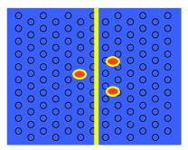
Figure 6: (color online). Three defect cavities coupled to one wave guide.

VI Thermalization of the coupled-cavity system

In this section, we consider the thermalization of the lossy driven atom-cavity system. For simplicity, we consider a simpler system which involves two defect cavities coupled to a driven wave guide, as shown in Fig. 7.

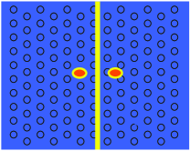
Figure 7: (color online). Two defect cavities coupled to one wave guide.

This system was studied in Ref. two-state , where the reservoir temperature is set to be zero and an analytical solution was obtained (see Eq. (23)-(29) therein). For finite temperature, the master equation needs to be modified, i.e. Eq. (12) and (13) of Ref. two-state are replaced by

$$L_{a}^{\prime}R= \kappa(n_{c}+1)(2aRa^{\dagger}-a^{\dagger}aR-Ra^{\dagger}a)+\kappa n_{c}(2a^{\dagger}Ra-aa^{\dagger}R-Raa^{\dagger}),$$ (23)

$$L_{p}^{\prime}R= \sum_{i=1}^{2}\gamma(n_{p}+1)(2\sigma_{i}R\sigma^{\dagger}_{i}-\sigma^{\dagger}_{i}\sigma_{i}R-\rho\sigma^{\dagger}_{i}\sigma_{i})+\gamma n_{p}(2\sigma^{\dagger}_{i}R\sigma-\sigma\sigma^{\dagger}_{i}R-R\sigma_{i}\sigma^{\dagger}_{i}),$$ (24)

where $n_{c}=\frac{1}{e^{\hbar\omega_{cav}/k_{B}T_{R}}-1}$ is the mean photon number at the reservoir temperature $T_{R}$ and the cavity frequency $\omega_{cav}$. Similarly $n_{p}=\frac{1}{e^{\hbar\omega_{pol}/k_{B}T_{R}}-1}$ is the mean photon number at the reservoir temperature $T_{R}$ and the polaritonic frequency $\omega_{pol}$.

The effective master equation for the two polaritons can be obtained using the same method in Ref. two-state . For $T_{R}\ll\hbar\omega_{pol}/k_{B}$, the temperature terms in Eq. (24) are preserved in the final effective master equation i.e. Eq. (20) of Ref. two-state . The steady state $\rho^{ss}$ is obtained by requiring $\frac{d\rho^{ss}}{dt}=0$. To characterize the degree of thermalization of the steady state, we calculate the distance between the steady state and a thermal state, using the following distance measure trace distance :

$$d(\rho^{ss},\,\,\rho^{th})=\frac{1}{2}\textrm{tr}|\rho^{ss}-\rho^{th}|.$$ (25)

The trace distance $d(\rho^{ss},\,\,\rho^{th})$ provides a useful measure to distinguish the steady state $\rho^{ss}$ from the thermal state $\rho^{th}$ through quantum measurements trace distance2 . Therefore, if $d(\rho^{ss},\,\,\rho^{th})$ increases with system parameters we say that the system is farther away from thermalization. Also, the thermal state $\rho^{th}$ is chosen to be $\rho^{th}=\exp[-\hbar\omega_{pol}(\sigma_{1}^{\dagger}\sigma_{1}+\sigma_{2}^{\dagger}\sigma_{2})/k_{B}T_{R}]$ up to a normalization factor tr$(\rho^{th})$.

Fig. 8 shows the distance $d(\rho^{ss},\,\,\rho^{th})$ as a function of $x$ and $T_{R}$, where $x$ is a parameter defined in Ref. two-state (below Eq. (22)) and it is proportional to the strength of the driving field. The relevant parameters $y=15,z=1.01$ (see Ref. two-state ). The unit of $T_{R}$ is $\hbar\omega_{pol}/k_{B}$. It is seen in Fig. 8 that the steady state is close to the thermal state if there is no driving field, and for stronger driving field the steady state is farther away from thermalization. This is reasonable from a physical perspective as the driving field generally induces coherence (i.e. non-zero off-diagonal elements in the polaritonic density matrix) for the polaritons while the thermal state is diagonal. In addition, it seems that $d(\rho^{ss},\,\,\rho^{th})$ does not depend on the reservoir temperature. This may be because $T_{R}\ll\hbar\omega_{pol}/k_{B}$ so that the effect of the thermal agitation is rather small. The effect should certainly manifest itself for larger $T_{R}$. However this regime is beyond the approximation for the derivation of the effective master equation ($T_{R}\ll\hbar\omega_{pol}/k_{B}$) and it is in general not easily solvable even with numerical calculations.

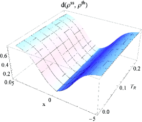
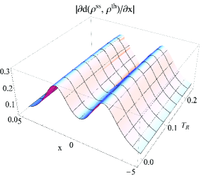
Figure 8: (color online). The distance $d(\rho^{ss},\,\,\rho^{th})$ for (a) and the derivative $|\partial d(\rho^{ss},\,\,\rho^{th})/\partial x|$ for (b) as functions of $x$ (proportional to the driving strength) and $T_{R}$.

Comparing Fig. 8 for a fixed $T_{R}$ with the first plot of Fig. 2 ($y=15$) in Ref. two-state , one finds that they are not consistent, especially for large $x$, for which $d(\rho^{ss},\,\,\rho^{th})$ is very large while the polaritonic entanglement is negligible. However, if one takes the derivative of $d(\rho^{ss},\,\,\rho^{th})$ with respect to $x$, then a relationship appears. Fig. 8 shows $|\partial d(\rho^{ss},\,\,\rho^{th})/\partial x|$ as a function of $x$ and $T_{R}$. It can be seen that there are two peaks for a fixed temperature. This is similar to the first plot of Fig. 2 in Ref. two-state . Also the two plots are consistent for large $x$. Therefore, it may be concluded that the change rate of the thermalization with respect to the driving strength (rather than the thermalization itself) is related to the polaritonic entanglement. Physically, for a increase/decrease of the driving strength i.e. more/less coherent energy is injected into the system, a more rapid change of the thermal property (or the degree of thermalization) of the system indicates that a stronger correlation (entanglement) is established. The coherent energy refers to fact that the driving field induces off-diagonal elements in the polaritonic density matrix as mentioned previously. One could conjecture that a more rapid change of the degree of thermalization of the system may indicate that the interaction between the two polaritons are stronger which leads to a stronger entanglement between them.

VII Conclusion

In this paper, we show that long-distance steady state entanglement in a lossy network of driven light-matter systems can be coherently controlled through the tuning of the phase difference between the driving fields. The role of driving phase field in engineering interaction and entanglement in coupled atom-cavities was also discussed in Ref. driving phase . Here, it is found that in a closed network of three-cavity-atom systems the maximum of entanglement for any pair is achieved even when their corresponding direct coupling is much smaller than their couplings to the third party. This effect is reminiscent of coherent effects found in quantum optics that coherent population transfers between otherwise uncoupled levels through a third level using two classical coherent fields. An alternative geometry: two-coupled cavities with three driving fields is discussed. For finite temperature, we analyze the thermalization of the two defect cavities coupled to one driven wave guide. It is found that the change rate of the thermalization of the system with respect to the driving strength (rather than the thermalization itself) can indicate the degree of the polaritonic correlation (entanglement).

Acknowledgement - This work was supported by National Research Foundation & Ministry of Education, Singapore. Li Dai would like to thank Dr. Jun-Hong An for helpful discussions.

References

- (1) D.G. Angelakis, et al., Phys. Lett. A 362, 377 (2007).
- (2) D.G. Angelakis, M.F. Santos and S. Bose, Phys. Rev. A, 76 (2007) R05709; A. Greentree et al., Nat. Phys., 2 (2006) 856; D. Rossini and R. Fazio, Phys. Rev. Lett., 99 (2007) 186401; M.X. Huo, Y. Li, Z. Song and C.P. Sun, Phys. Rev. A, 77 022103 (2008); Y.C. Neil Na et al., Phys. Rev. A, 77 031803(R)(2008); M. Paternostro, G.S. Agarwal and M.S. Kim, arXiv:0707.0846; E.K. Irish, C.D. Ogden and M.S. Kim, Phys. Rev. A, 77, 033801 (2008).
- (3) D. G. Angelakis, S. Bose and S. Mancini, Europhys. Lett., 85, 20007 (2009).
- (4) M. B. Plenio and S.F. Huelga Phys. Rev. Lett. 88, 197901 (2002); M. J. Hartmann and M.B. Plenio, Phys. Rev. Lett. 101, 200503 (2008).
- (5) Dario Gerace. et al., Nat. Phys., 5, 281 (2009); A. Tomadin et al., arXiv:0904.4437; I. Carusotto, et al., Phys. Rev. Lett., 103, 033601 (2009).
- (6) H.J. Carmichael, Statistical methods in quantum optics. 1, Master equations and Fokker-Planck equations, New York: Springer, 1999.
- (7) J. P. Reithmaier, et al., Nature, 432, 197 (2004); H. Altug and J. Vuckovic, App. Phys. Lett. 84, 161 (2004); T. Yoshie, , et al., Nature, 432, 200 (2004); K. Hennessy, et al., Nature, 445, 896 (2007); E. Peter, et al., Phys. Rev. Lett. 95, 067401 (2005); David Press, et al., Phys. Rev. Lett. 98, 117402 (2007).
- (8) Takao Aoki, et al., Nature, 443, 671 (2006); Trupke M. et al., Phys. Rev. Lett., 99, 063601 (2007); Majer J. et al., Nature, 449, 443 (2007).
- (9) Stephen M. Barnett and Paul M. Radmore, Methods in theoretical quantum optics, New York, Clarendon Press, 1997.
- (10) H.-P. Breuer and F. Petruccione, The theory of open quantum systems, Oxford University Press, 2002.
- (11) W. K. Wootters, Phys. Rev. Lett. 80, 2245 (1998).
- (12) M. O. Scully and M. S. Zubairy, Quantum Optics, Cambridge University Press, 1997.
- (13) K. -J. Boller, A. Imamoglu, and S. E. Harris, Phys. Rev. Lett., 66 2593 (1991).
- (14) M. A. Nielsen and I. C. Chuang, Quantum Computation and Quantum Information, Cambridge University Press, 2000.
- (15) Sandu Popescu, Anthony J. Short, and Andreas Winter, Nature Physics 2, 754 (2006).
- (16) S. Mancini and S. Bose, Phys. Rev. A, 70, 022307 (2004).