Dynamical transition of glasses: from exact to approximate.

Abstract

We introduce a family of glassy models having a parameter, playing the role of an interaction range, that may be varied continuously to go from a system of particles in $\displaystyle d$ dimensions to a mean-field version of it. The mean-field limit is exactly described by equations conceptually close, but different from, the Mode-Coupling equations. We obtain these by a dynamic virial construction. Quite surprisingly we observe that in three dimensions, the mean-field behavior is closely followed for ranges as small as one interparticle distance, and still qualitatively for smaller distances. For the original particle model, we expect the present mean-field theory to become, unlike the Mode-Coupling equations, an increasingly good approximation at higher dimensions.

In the past few years, there has been considerable activity on the application of Mode-Coupling theory to liquid systems. In its original conception, Mode Coupling is an approximation for the dynamics in which an (infinite) subset of corrections coming from non-linearities is taken into account. The theory has become popular not so much for the accuracy of its predictions – numerical confirmation often demands considerably good will to accept – but because it gives a unified and qualitative view of the first steps of the slowing down of dynamics, as the system approaches the glass transition.

Mode-Coupling theory was originally confined to the dynamics in equilibrium liquid phase. However, similar approximations may be applied to the equilibrium statistical mechanics of systems above and below the glass transition, and to the non-equilibrium (”aging”) dynamics below the glass transition. Elaborating on an idea of Kraichnan kraichnan1962stochastic1 , Kirkpatick, Thirumalai and Wolynes PhysRevLett.58.2091 ; PhysRevB.36.5388 ; kirkpatrick1987connections noted that one may view these approximate theories as being the exact description of the properties of an auxiliary model, different from the original one. These turn out to be disordered models having nature that is ‘mean-field’ in the following sense: if a particle (or spin) $\displaystyle\bf A$ interacts strongly with two other particles $\displaystyle\bf B$ and $\displaystyle\bf C$, then $\displaystyle\bf B$ and $\displaystyle\bf C$ do not interact strongly with one another. This may happen either because the network of interactions is tree-like, or because all individual interactions are weak.

There is a large family of such ‘mean-field’ models, going beyond the one that leads to the original mode-coupling equations, and they may all be treated with the tools developed in the context of spin glass theory. When applied to the glass transition, the whole strategy is referred to as ”Random First Order” scenario: a single name for approximation schemes that may be different is justified because the expectation is that the nature of the glass transition, of the equilibrium glass phase, and of the out of equilibrium dynamics, is qualitatively the same in all these mean-field models. The wider question whether this scenario holds strictly at finite dimensions is still very far from established.

Once one recognizes that Mode-Coupling is a form of mean-field theory, the first instinct is to ask under which conditions it becomes exact, in particular if it does so in high dimensions. The answer for the latter question is that it does not PhysRevLett.104.255704 . This lack of control over the approximation is problematic, because there is no unambiguous way of relating features of a realistic system with those of the Mode-Coupling solution – and we often are not sure whether some qualitative crossover in the behavior of an experimental system should be associated with the idealized Mode-Coupling transition, and in what sense.

In this paper we study an approximation of the same general mean-field class than, but different from, the one leading to the mode-coupling equations. In order to bridge the gap between this limit and reality, we build explicit models where an interaction range is tuned by some parameter, thus allowing to go continuously from mean-field to true finite-dimensions by varying this parameter. Work in this direction already exist for spin glasses  frohlich1987some ; franz2004finite ; franz2004kac ; sarlat2009these , where one can consider models with interactions with tunable range, as originally proposed by Kac. As we shall mention below, for particle systems, the usual program à la Kac meets a problem as the interactions are made longer in range and less strong: at low temperatures and large densities particles tend to arrange themselves in clusters grewe1977kirkwood2 ; klein1994repulsive ; mel1995long , themselves arranged in a crystalline or amorphous ‘mesophase’ structure. Thus, it seems that in order to prevent this, one is forced to add a short-range hard-core repulsion, thus spoiling the Kac (mean-field) nature of the model. In this paper we follow a different path, based on a suggestion already made by Kraichnan fifty years ago: we study particles with short-range interactions which are, however, ‘shifted’ by a random amount having a typical range, which is our parameter.

Within this framework we are able to address several issues related to the glass transition, revisiting them via the mean-field model we introduce. As an example, we are able to answer questions such as: ”what is the relation between the point at which the dynamics becomes nonexponential and the dynamic transition”, because we can continuously take the model from finite dimensional to a mean-field limit, a situation where both transition points are well-defined, independently of any fitting procedure.

This paper is divided in two parts, analytic and numeric, which may be read independently. Sections II and III are devoted to the analytic treatment of the statics and the dynamics of the liquid phase, respectively. The main new result is an equation for the dynamics that plays the role of the mode-coupling equation, and is exact in the mean-field limit. Sections IV and V present the numerical tests for statics and dynamics, respectively. We are able to compare the results in the mean-field limit with the ones for finite parameter $\displaystyle\lambda$, all the way down to the ordinary particle model $\displaystyle\lambda=0$. In section VI we discuss an instance where having an approximation with some limit in which it is well controlled is reassuring: there has been some doubt whether the so-called ”onset temperature” (or pressure) sastry1998signatures , at which the equilibrium dynamics becomes nonexponential (and the inherent structures start to have deep energies), should be identified with the mode-coupling transition. Here, by taking continuously the parameter $\displaystyle\lambda$ to infinity, we find that they are in fact two distinct pressures – at least in the limit in which they are both well defined.

I Model

I.1 Kac models, clustering and the Kirkwood instability

One can introduce a mean-field treatment of particle systems in different ways. One may, for example, use explicit infinite range interactions dotsenko2004infinite ; dotsenko2005mean . Glassiness is obtained by choosing a potential imposing a strong frustration, and there is in principle no need for quenched disorder. Next, one may consider long, but finite ranges, in the spirit of Kac interactions. Although quite intuitive, the choice of the potential is in practice difficult, as crystallization gils2007absence or instabilities in the liquid phase (like the Kirkwood instability kirkwood1941statistical ; grewe1977kirkwood2 ; klein1994repulsive ; mel1995long ; likos2007ultrasoft ; fragner2007interparticle ) easily set in as soon as the interaction range is finite.

Consider, for example, the model studied by Dotsenko dotsenko2004infinite ; dotsenko2005mean . Particles are in a confining potential $\displaystyle V_{conf}({\bf x_{a}})$ (which may be harmonic) and interact with a long-range, oscillatory potential:

$$H=\frac{1}{\sqrt{N}}\sum_{a\neq b}\cos(|{\bf x_{a}}-{\bf x_{b}}|)+\sum_{a}V_{conf}({\bf x_{a}})$$ (1)

Dotsenko showed that the system indeed has a mean-field glass phase, induced by the frustration due to the conflict of attraction and repulsion. The next step, in an ordinary Kac program, would be to introduce the model with a finite range $\displaystyle\gamma$:

$$H=\frac{1}{\sqrt{\gamma}}\sum_{a\neq b}\cos(|{\bf x_{a}}-{\bf x_{b}}|)e^{-|{\bf x_{a}}-{\bf x_{b}}|/\gamma}+\sum_{a}V_{conf}({\bf x_{a}})$$ (2)

The result is disappointing: instead of giving a glass, the system arranges as follows: it forms clusters of many particles, themselves disposed in a crystalline arrangement, at the optimal distance so that the interaction between clusters is minimized. The way to avoid the crystal-of-clusters mesophase is, of course, to add a hard-core that hampers the clustering, but then the model is no longer mean field. Another related difficulty with this strategy is that even the liquid phase may have a transition to a ‘liquid’ with spatial modulation, the Kirkwood instability kirkwood1941statistical ; grewe1977kirkwood2 ; klein1994repulsive ; mel1995long . This phase is not without interest of its own (see Fig. 3 for a numerical simulation), but it is not what we are wishing to study here.

Another way to construct a mean-field model is to work with particles on a Bethe lattice PhysRevE.67.057105 ; rivoire2003glass ; PhysRevLett.88.025501 ; tarzia2004glass ; mari2009jamming . This introduces quenched disorder and the mean-field nature at the same time. By increasing the graph connectivity, one can, at least formally, recover the original finite dimensional model by setting the graph connectivity to infinity.

I.2 Kraichnan’s proposal and beyond.

In this paper, we will follow another route. We study family of models which are defined through the Hamiltonian:

$$H(\{\mathbf{x}\},\{\mathbf{A}\})=\sum_{<i,j>}V(\mathbf{x_{i}}-\mathbf{x_{j}}-\mathbf{A_{ij}})$$ (3)

where $\displaystyle V$ is a short-ranged interaction potential. The $\displaystyle\mathbf{x}$’s are the positions of the particles and the $\displaystyle\mathbf{A}$’s are quenched random variables with a probability distribution $\displaystyle P(|\mathbf{A}|)$, which has a variance $\displaystyle\lambda^{2}$. We also impose that $\displaystyle\mathbf{A}_{ij}=\mathbf{A}_{ji}$. The model for $\displaystyle\lambda=\infty$ was first introduced by Kraichnan some fifty years ago kraichnan1962stochastic1 .

When $\displaystyle\lambda=0$, $\displaystyle P(|\mathbf{A}|)=\delta(|\mathbf{A}|)$, and the model reduces to an usual $\displaystyle d$-dimensional system. On the other hand, when $\displaystyle\lambda\to\infty$, one particle $\displaystyle i$ can interact with particles $\displaystyle j$ which are possibly anywhere in the system, as long as $\displaystyle|\mathbf{x_{i}}-\mathbf{x_{j}}-\mathbf{A_{ij}}|$ is of the order of the range of the potential $\displaystyle V$. Therefore, the system tends to have a mean-field nature in this limit even though one particle effectively interacts with a finite number of other particles, as it does in a conventional finite-dimensional hard sphere system (see Fig. 1). Thus by tuning $\displaystyle\lambda$, the model (3) goes from a finite dimensional system ($\displaystyle\lambda=0$) to a mean-field realization of the same system ($\displaystyle\lambda\to\infty$).

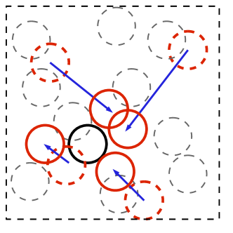
Figure 1: The black particle effectively interacts with a finite number of particles (in red) that have appropriate random shifts (blue arrows), but these particles may be anywhere in the sample.

In the liquid phase, the mean-field limit of the model has an entropy of an ideal gas plus only the first virial correction, just like a van der Waals gas. Physically, this comes from the fact that it is very unlikely that three (or more) spheres effectively interact simultaneously with one another, as is sketched in Fig. 2. For instance, in the hard-sphere case, one would need to have, for particles $\displaystyle i$, $\displaystyle j$, and $\displaystyle k$ (having a diameter $\displaystyle D$):

$$\begin{array}[]{c}|\mathbf{x_{i}}-\mathbf{x_{j}}-\mathbf{A_{ij}}|\sim D\\ |\mathbf{x_{j}}-\mathbf{x_{k}}-\mathbf{A_{jk}}|\sim D\\ |\mathbf{x_{k}}-\mathbf{x_{i}}-\mathbf{A_{ki}}|\sim D\end{array}$$ (4)

which requires that the random shifts satisfy $\displaystyle|\mathbf{A_{ij}}+\mathbf{A_{jk}}+\mathbf{A_{ki}}|\sim D$. This of course is very unlikely for shifts $\displaystyle|\mathbf{A}|\sim L$, where $\displaystyle L$ is the linear size of the system.

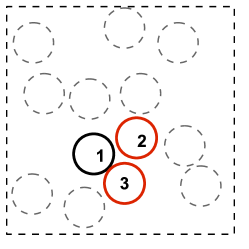
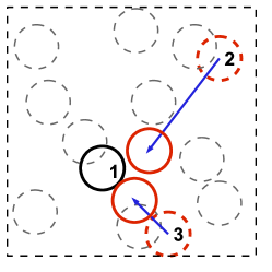
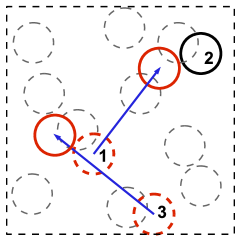
Figure 2: Left : Effective three-body correlation in a finite-dimensional hard-sphere system (with no random shifts), leading to corrections beyond the first virial term. Center : Same situation in the random shift model, from the point of view of particle 1. Particle 1 sees particles 2 and 3 nearby. Right : From the point of view of particle 2, there is no effective three-body interaction, as the random shifts displaces particle 3 very far from particle 2.

In this work, we will concentrate mostly on the hard-sphere potential, but the procedure is a very generic way to obtain a mean-field limit, and can even be generalized to objects with rotational degrees of freedom, where one can introduce a rotational disorder. We studied both a monodisperse system, for conceptual simplicity; and a bidisperse one, to be able to work with arbitrary small $\displaystyle\lambda$ without having to deal with crystallisation.

From now on, we set the diameter $\displaystyle D$ of a sphere (in the monodisperse case) to $\displaystyle D=1$, which will be used as length scale. The temperature $\displaystyle T$ is set to $\displaystyle 1$ almost everywhere, as it is irrelevant for hard spheres. The only part where we keep it explicit is in the section dealing with the dynamics of the model. For simplicity we introduce the following notations: a sphere with diameter $\displaystyle 1$ in dimension $\displaystyle d$ has a volume $\displaystyle 2^{-d}v_{d}$, and a surface $\displaystyle s_{d}$.

II Statics of the liquid phase

II.1 Grand-canonical formalism and Mayer expansion

In this section, we work with a monodisperse system. We note $\displaystyle V(u)$ the interaction potential:

$$\begin{array}[]{r|l}\hbox{\multirowsetup V(u)=}&\infty\quad\text{if}\quad u>1\\ &0\quad\text{otherwise}\end{array}$$ (5)

The canonical partition function of the system reads:

$$Z_{\{\mathbf{A}\}}=\int\prod_{k}d\mathbf{x_{k}}\exp\left(-\sum_{ij}V(\mathbf{x_{i}}-\mathbf{x_{j}}-\mathbf{A_{ij}})\right)$$ (6)

One would like to study the entropy of the system averaged over disorder:

$$S=-\overline{\ln Z_{\{\mathbf{A}\}}}$$ (7)

In the liquid phase, we can treat this average as an annealed average over the disorder:

$$S=S_{an}=-\ln\overline{Z_{\{\mathbf{A}\}}}$$ (8)

So the problem reduces to the study of:

$$\overline{Z_{\{\mathbf{A}\}}}=\frac{1}{N!}\int\prod_{lm}P(\mathbf{A}_{lm})d\mathbf{A}_{lm}\int\prod_{k}d\mathbf{x_{k}}\exp\left(-\sum_{ij}V(\mathbf{x_{i}}-\mathbf{x_{j}}-\mathbf{A_{ij}})\right)$$ (9)

We introduced a $\displaystyle 1/N!$ prefactor to be able to perform the next step, a Mayer expansion. We just have to remember to compensate this factor at the end of the computation. To do the Mayer expansion, we have to translate our problem in a grand-canonical formalism. We introduce the grand-canonical partition function:

$$\overline{\Theta}=\sum_{N}z^{N}\overline{Z_{\{\mathbf{A}\}}}$$ (10)

where $\displaystyle z$ is the activity, related to the chemical potential $\displaystyle\mu$ by $\displaystyle z=e^{\mu}$, and we rewrite Eq. (9) as:

$$\overline{Z_{\{\mathbf{A}\}}}=\int\prod_{k}d\mathbf{x_{k}}\prod_{ij}\left[\overline{f}(\mathbf{x_{i}}-\mathbf{x_{j}})+1\right]$$ (11)

where $\displaystyle\overline{f}$ is an annealed Mayer function:

$$\overline{f}(\mathbf{x}-\mathbf{y})=\int d\mathbf{A}P(\mathbf{A})\left[\exp\left(-V(\mathbf{x}-\mathbf{y}-\mathbf{A})\right)-1\right]=-\int d\mathbf{A}P(\mathbf{A})\chi(|\mathbf{x}-\mathbf{y}-\mathbf{A}|)$$ (12)

with $\displaystyle\chi(r)$ the step function such that $\displaystyle\chi(r)=1$ if $\displaystyle r<1$ and $\displaystyle\chi(r)=0$ otherwise. We can then introduce a diagrammatic representation to express the grand-canonical potential $\displaystyle G=\ln\overline{\Theta}$ as usualhansen2006theory :

$$\begin{array}[b]{lllll}G=\ln\overline{\Theta}=\{\text{ connected diagrams }\}=\lx@xy@svg{\hbox{\raise 0.0pt\hbox{\kern 5.5pt\hbox{\ignorespaces\ignorespaces\ignorespaces\hbox{\vtop{\kern 0.0pt\offinterlineskip\halign{\entry@#!@&&\entry@@#!@\cr\crcr}}}\ignorespaces{\hbox{\kern-5.5pt\raise 0.0pt\hbox{\hbox{\kern 0.0pt\raise 0.0pt\hbox{\hbox{\kern 3.0pt\raise 0.0pt\hbox{$\displaystyle\textstyle{\bullet}$}}}}}}}\ignorespaces}}}}\ignorespaces+&\hskip 2.27626pt\pbox[c]{2cm}{\lx@xy@svg{\hbox{\raise 0.0pt\hbox{\kern 0.0pt\hbox{\ignorespaces\ignorespaces\ignorespaces\hbox{\vtop{\kern 0.0pt\offinterlineskip\halign{\entry@#!@&&\entry@@#!@\cr&\crcr}}}\ignorespaces{\hbox{\kern 0.0pt\raise 0.0pt\hbox{\hbox{\kern-2.5pt\raise-2.22223pt\hbox{$\displaystyle\textstyle{\bullet}$}}}}}\ignorespaces{\hbox{\kern 15.5pt\raise 0.0pt\hbox{\hbox{\kern 0.0pt\raise-2.22223pt\hbox{$\displaystyle\textstyle{\bullet}$}}}}}\ignorespaces\ignorespaces\ignorespaces{}{\hbox{\lx@xy@droprule}}\ignorespaces{}{\hbox{\lx@xy@droprule}}{\hbox{\lx@xy@droprule}}{\hbox{\kern 15.0pt\raise 0.0pt\hbox{\hbox{\kern 0.0pt\raise 0.0pt\hbox{\hbox{\kern 3.0pt\raise 0.0pt\hbox{$\displaystyle\textstyle{}$}}}}}}}\ignorespaces}}}}\ignorespaces}+&\pbox[c]{2cm}{\lx@xy@svg{\hbox{\raise 0.0pt\hbox{\kern 3.0pt\hbox{\ignorespaces\ignorespaces\ignorespaces\hbox{\vtop{\kern 0.0pt\offinterlineskip\halign{\entry@#!@&&\entry@@#!@\cr&\\&&\crcr}}}\ignorespaces{\hbox{\kern-3.0pt\raise 0.0pt\hbox{\hbox{\kern 0.0pt\raise 0.0pt\hbox{\hbox{\kern 3.0pt\raise 0.0pt\hbox{$\displaystyle\textstyle{}$}}}}}}}{\hbox{\kern 9.0pt\raise 0.0pt\hbox{\hbox{\kern-2.5pt\raise-2.22223pt\hbox{$\displaystyle\textstyle{\bullet}$}}}}}\ignorespaces{\hbox{\kern 15.0pt\raise-12.0pt\hbox{\hbox{\kern 0.0pt\raise-2.22223pt\hbox{$\displaystyle\textstyle{\bullet}$}}}}}\ignorespaces\ignorespaces{}\ignorespaces\ignorespaces{\hbox{\lx@xy@drawline@}}\ignorespaces{}\ignorespaces\ignorespaces{\hbox{\lx@xy@drawline@}}\ignorespaces{\hbox{\lx@xy@drawline@}}\ignorespaces{\hbox{\kern-2.5pt\raise-12.0pt\hbox{\hbox{\kern 0.0pt\raise-2.22223pt\hbox{$\displaystyle\textstyle{\bullet}$}}}}}\ignorespaces\ignorespaces{}\ignorespaces\ignorespaces{\hbox{\lx@xy@drawline@}}\ignorespaces{}\ignorespaces\ignorespaces{\hbox{\lx@xy@drawline@}}\ignorespaces{\hbox{\lx@xy@drawline@}}{\hbox{\kern 0.0pt\raise-12.0pt\hbox{\hbox{\kern-2.5pt\raise-2.22223pt\hbox{$\displaystyle\textstyle{\bullet}$}}}}}{\hbox{\kern 6.0pt\raise-12.0pt\hbox{\hbox{\kern 0.0pt\raise 0.0pt\hbox{\hbox{\kern 3.0pt\raise 0.0pt\hbox{$\displaystyle\textstyle{}$}}}}}}}{\hbox{\kern 15.0pt\raise-12.0pt\hbox{\hbox{\kern 0.0pt\raise-2.22223pt\hbox{$\displaystyle\textstyle{\bullet}$}}}}}\ignorespaces}}}}\ignorespaces}+&\pbox[c]{2cm}{\lx@xy@svg{\hbox{\raise 0.0pt\hbox{\kern 3.0pt\hbox{\ignorespaces\ignorespaces\ignorespaces\hbox{\vtop{\kern 0.0pt\offinterlineskip\halign{\entry@#!@&&\entry@@#!@\cr&\\&&\crcr}}}\ignorespaces{\hbox{\kern-3.0pt\raise 0.0pt\hbox{\hbox{\kern 0.0pt\raise 0.0pt\hbox{\hbox{\kern 3.0pt\raise 0.0pt\hbox{$\displaystyle\textstyle{}$}}}}}}}{\hbox{\kern 9.0pt\raise 0.0pt\hbox{\hbox{\kern-2.5pt\raise-2.22223pt\hbox{$\displaystyle\textstyle{\bullet}$}}}}}\ignorespaces{\hbox{\kern 15.5pt\raise-12.0pt\hbox{\hbox{\kern 0.0pt\raise-2.22223pt\hbox{$\displaystyle\textstyle{\bullet}$}}}}}\ignorespaces\ignorespaces{}\ignorespaces\ignorespaces{\hbox{\lx@xy@drawline@}}\ignorespaces{}\ignorespaces\ignorespaces{\hbox{\lx@xy@drawline@}}\ignorespaces{\hbox{\lx@xy@drawline@}}\ignorespaces{\hbox{\kern-2.5pt\raise-12.0pt\hbox{\hbox{\kern 0.0pt\raise-2.22223pt\hbox{$\displaystyle\textstyle{\bullet}$}}}}}\ignorespaces\ignorespaces{}\ignorespaces\ignorespaces{\hbox{\lx@xy@drawline@}}\ignorespaces{}\ignorespaces\ignorespaces{\hbox{\lx@xy@drawline@}}\ignorespaces{\hbox{\lx@xy@drawline@}}{\hbox{\kern 0.0pt\raise-12.0pt\hbox{\hbox{\kern-2.5pt\raise-2.22223pt\hbox{$\displaystyle\textstyle{\bullet}$}}}}}\ignorespaces{\hbox{\kern 15.5pt\raise-12.0pt\hbox{\hbox{\kern 0.0pt\raise-2.22223pt\hbox{$\displaystyle\textstyle{\bullet}$}}}}}\ignorespaces\ignorespaces\ignorespaces{}{\hbox{\lx@xy@droprule}}\ignorespaces{}{\hbox{\lx@xy@droprule}}{\hbox{\lx@xy@droprule}}{\hbox{\kern 6.0pt\raise-12.0pt\hbox{\hbox{\kern 0.0pt\raise 0.0pt\hbox{\hbox{\kern 3.0pt\raise 0.0pt\hbox{$\displaystyle\textstyle{}$}}}}}}}{\hbox{\kern 15.0pt\raise-12.0pt\hbox{\hbox{\kern 0.0pt\raise 0.0pt\hbox{\hbox{\kern 3.0pt\raise 0.0pt\hbox{$\displaystyle\textstyle{}$}}}}}}}\ignorespaces}}}}\ignorespaces}+&\dots\end{array} \textstyle{\bullet} \textstyle{\bullet} \textstyle{\bullet} \textstyle{\bullet} \textstyle{\bullet} \textstyle{\bullet} \textstyle{\bullet} \textstyle{\bullet} \textstyle{\bullet} \textstyle{\bullet} \textstyle{\bullet} \textstyle{\bullet} \textstyle{\bullet} \textstyle{\bullet} \textstyle{\bullet} \textstyle{\bullet} \textstyle{\bullet} \textstyle{\bullet} \textstyle{\bullet} \textstyle{\bullet} \textstyle{\bullet} \textstyle{\bullet} \textstyle{\bullet} \textstyle{\bullet} \textstyle{\bullet} \textstyle{\bullet}$$ (13)

where the diagram vertices represent a factor $\displaystyle z$ while the bonds represent the Mayer function $\displaystyle\overline{f}$.

II.2 Mean-field equation of state

As already noted by Kraichnan kraichnan1962stochastic1 , only the first virial correction survives in the mean-field limit. The entropy can then be expressed in term of the density field $\displaystyle\rho(\mathbf{x})$:

$$S_{an}[\rho(\mathbf{x})]=-\int\text{d}\mathbf{x}\rho(\mathbf{x})\left[\ln\rho(\mathbf{x})-1\right]+\frac{1}{2}\int\text{d}\mathbf{x}\text{d}\mathbf{y}\rho(\mathbf{x})\rho(\mathbf{y})\overline{f}(\mathbf{x}-\mathbf{y})+N\ln N$$ (14)

The $\displaystyle\ln N$ contribution to the entropy density reflects the fact that particles are not, in this model, truly indistinguishable – just as they are not in a system particles of polydisperse sizes.

The fact that the first terms contribute can be understood by noticing that:

$$\overline{f}(\mathbf{x}-\mathbf{y})=-v_{d}/V$$ (15)

Thus, in the Mayer expansion Eq (13), a diagram with $\displaystyle n$ vertices and $\displaystyle m$ bonds reads $\displaystyle V^{n-m}z^{n}(-v_{d})^{m}$. If $\displaystyle m\geq n$, the diagram vanishes in the thermodynamic limit, because this requires that several random shifts add to zero. Only the diagrams having $\displaystyle m<n$ contribute, and they are the tree ones (having $\displaystyle m=n-1$):

$$\ln\overline{\Theta}=\lx@xy@svg{\hbox{\raise 0.0pt\hbox{\kern 5.5pt\hbox{\ignorespaces\ignorespaces\ignorespaces\hbox{\vtop{\kern 0.0pt\offinterlineskip\halign{\entry@#!@&&\entry@@#!@\cr\crcr}}}\ignorespaces{\hbox{\kern-5.5pt\raise 0.0pt\hbox{\hbox{\kern 0.0pt\raise 0.0pt\hbox{\hbox{\kern 3.0pt\raise 0.0pt\hbox{$\displaystyle\textstyle{\bullet}$}}}}}}}\ignorespaces}}}}\ignorespaces+\hskip 2.27626pt\pbox[c]{2cm}{\lx@xy@svg{\hbox{\raise 0.0pt\hbox{\kern 0.0pt\hbox{\ignorespaces\ignorespaces\ignorespaces\hbox{\vtop{\kern 0.0pt\offinterlineskip\halign{\entry@#!@&&\entry@@#!@\cr&\crcr}}}\ignorespaces{\hbox{\kern 0.0pt\raise 0.0pt\hbox{\hbox{\kern-2.5pt\raise-2.22223pt\hbox{$\displaystyle\textstyle{\bullet}$}}}}}\ignorespaces{\hbox{\kern 15.5pt\raise 0.0pt\hbox{\hbox{\kern 0.0pt\raise-2.22223pt\hbox{$\displaystyle\textstyle{\bullet}$}}}}}\ignorespaces\ignorespaces\ignorespaces{}{\hbox{\lx@xy@droprule}}\ignorespaces{}{\hbox{\lx@xy@droprule}}{\hbox{\lx@xy@droprule}}{\hbox{\kern 15.0pt\raise 0.0pt\hbox{\hbox{\kern 0.0pt\raise 0.0pt\hbox{\hbox{\kern 3.0pt\raise 0.0pt\hbox{$\displaystyle\textstyle{}$}}}}}}}\ignorespaces}}}}\ignorespaces}+\pbox[c]{2cm}{\lx@xy@svg{\hbox{\raise 0.0pt\hbox{\kern 3.0pt\hbox{\ignorespaces\ignorespaces\ignorespaces\hbox{\vtop{\kern 0.0pt\offinterlineskip\halign{\entry@#!@&&\entry@@#!@\cr&\\&&\crcr}}}\ignorespaces{\hbox{\kern-3.0pt\raise 0.0pt\hbox{\hbox{\kern 0.0pt\raise 0.0pt\hbox{\hbox{\kern 3.0pt\raise 0.0pt\hbox{$\displaystyle\textstyle{}$}}}}}}}{\hbox{\kern 9.0pt\raise 0.0pt\hbox{\hbox{\kern-2.5pt\raise-2.22223pt\hbox{$\displaystyle\textstyle{\bullet}$}}}}}\ignorespaces{\hbox{\kern 15.0pt\raise-12.0pt\hbox{\hbox{\kern 0.0pt\raise-2.22223pt\hbox{$\displaystyle\textstyle{\bullet}$}}}}}\ignorespaces\ignorespaces{}\ignorespaces\ignorespaces{\hbox{\lx@xy@drawline@}}\ignorespaces{}\ignorespaces\ignorespaces{\hbox{\lx@xy@drawline@}}\ignorespaces{\hbox{\lx@xy@drawline@}}\ignorespaces{\hbox{\kern-2.5pt\raise-12.0pt\hbox{\hbox{\kern 0.0pt\raise-2.22223pt\hbox{$\displaystyle\textstyle{\bullet}$}}}}}\ignorespaces\ignorespaces{}\ignorespaces\ignorespaces{\hbox{\lx@xy@drawline@}}\ignorespaces{}\ignorespaces\ignorespaces{\hbox{\lx@xy@drawline@}}\ignorespaces{\hbox{\lx@xy@drawline@}}{\hbox{\kern 0.0pt\raise-12.0pt\hbox{\hbox{\kern-2.5pt\raise-2.22223pt\hbox{$\displaystyle\textstyle{\bullet}$}}}}}{\hbox{\kern 6.0pt\raise-12.0pt\hbox{\hbox{\kern 0.0pt\raise 0.0pt\hbox{\hbox{\kern 3.0pt\raise 0.0pt\hbox{$\displaystyle\textstyle{}$}}}}}}}{\hbox{\kern 15.0pt\raise-12.0pt\hbox{\hbox{\kern 0.0pt\raise-2.22223pt\hbox{$\displaystyle\textstyle{\bullet}$}}}}}\ignorespaces}}}}\ignorespaces}+\pbox[c]{2cm}{\lx@xy@svg{\hbox{\raise 0.0pt\hbox{\kern 2.5pt\hbox{\ignorespaces\ignorespaces\ignorespaces\hbox{\vtop{\kern 0.0pt\offinterlineskip\halign{\entry@#!@&&\entry@@#!@\cr&\\&\crcr}}}\ignorespaces{\hbox{\kern 0.0pt\raise 0.0pt\hbox{\hbox{\kern-2.5pt\raise-2.22223pt\hbox{$\displaystyle\textstyle{\bullet}$}}}}}\ignorespaces{\hbox{\kern-2.5pt\raise-18.0pt\hbox{\hbox{\kern 0.0pt\raise-2.22223pt\hbox{$\displaystyle\textstyle{\bullet}$}}}}}\ignorespaces\ignorespaces\ignorespaces{}{\hbox{\lx@xy@droprule}}\ignorespaces{}{\hbox{\lx@xy@droprule}}{\hbox{\lx@xy@droprule}}\ignorespaces{\hbox{\kern 15.5pt\raise 0.0pt\hbox{\hbox{\kern 0.0pt\raise-2.22223pt\hbox{$\displaystyle\textstyle{\bullet}$}}}}}\ignorespaces\ignorespaces\ignorespaces{}{\hbox{\lx@xy@droprule}}\ignorespaces{}{\hbox{\lx@xy@droprule}}{\hbox{\lx@xy@droprule}}{\hbox{\kern 18.0pt\raise 0.0pt\hbox{\hbox{\kern-2.5pt\raise-2.22223pt\hbox{$\displaystyle\textstyle{\bullet}$}}}}}\ignorespaces{\hbox{\kern 15.5pt\raise-18.0pt\hbox{\hbox{\kern 0.0pt\raise-2.22223pt\hbox{$\displaystyle\textstyle{\bullet}$}}}}}\ignorespaces\ignorespaces\ignorespaces{}{\hbox{\lx@xy@droprule}}\ignorespaces{}{\hbox{\lx@xy@droprule}}{\hbox{\lx@xy@droprule}}{\hbox{\kern-2.5pt\raise-18.0pt\hbox{\hbox{\kern 0.0pt\raise-2.22223pt\hbox{$\displaystyle\textstyle{\bullet}$}}}}}{\hbox{\kern 15.5pt\raise-18.0pt\hbox{\hbox{\kern 0.0pt\raise-2.22223pt\hbox{$\displaystyle\textstyle{\bullet}$}}}}}\ignorespaces}}}}\ignorespaces}+\pbox[c]{2cm}{\lx@xy@svg{\hbox{\raise 0.0pt\hbox{\kern 3.0pt\hbox{\ignorespaces\ignorespaces\ignorespaces\hbox{\vtop{\kern 0.0pt\offinterlineskip\halign{\entry@#!@&&\entry@@#!@\cr&\\&&\crcr}}}\ignorespaces{\hbox{\kern-3.0pt\raise 0.0pt\hbox{\hbox{\kern 0.0pt\raise 0.0pt\hbox{\hbox{\kern 3.0pt\raise 0.0pt\hbox{$\displaystyle\textstyle{}$}}}}}}}{\hbox{\kern 8.5pt\raise 0.0pt\hbox{\hbox{\kern-2.5pt\raise-2.22223pt\hbox{$\displaystyle\textstyle{\bullet}$}}}}}\ignorespaces{\hbox{\kern 14.0pt\raise-11.22221pt\hbox{\hbox{\kern 0.0pt\raise-2.22223pt\hbox{$\displaystyle\textstyle{\bullet}$}}}}}\ignorespaces\ignorespaces{}\ignorespaces\ignorespaces{\hbox{\lx@xy@drawline@}}\ignorespaces{}\ignorespaces\ignorespaces{\hbox{\lx@xy@drawline@}}\ignorespaces{\hbox{\lx@xy@drawline@}}\ignorespaces{\hbox{\kern 6.0pt\raise-11.22221pt\hbox{\hbox{\kern 0.0pt\raise-2.22223pt\hbox{$\displaystyle\textstyle{\bullet}$}}}}}\ignorespaces\ignorespaces\ignorespaces{}{\hbox{\lx@xy@droprule}}\ignorespaces{}{\hbox{\lx@xy@droprule}}{\hbox{\lx@xy@droprule}}\ignorespaces{\hbox{\kern-2.5pt\raise-11.22221pt\hbox{\hbox{\kern 0.0pt\raise-2.22223pt\hbox{$\displaystyle\textstyle{\bullet}$}}}}}\ignorespaces\ignorespaces{}\ignorespaces\ignorespaces{\hbox{\lx@xy@drawline@}}\ignorespaces{}\ignorespaces\ignorespaces{\hbox{\lx@xy@drawline@}}\ignorespaces{\hbox{\lx@xy@drawline@}}{\hbox{\kern 0.0pt\raise-11.22221pt\hbox{\hbox{\kern-2.5pt\raise-2.22223pt\hbox{$\displaystyle\textstyle{\bullet}$}}}}}{\hbox{\kern 6.0pt\raise-11.22221pt\hbox{\hbox{\kern 0.0pt\raise-2.22223pt\hbox{$\displaystyle\textstyle{\bullet}$}}}}}{\hbox{\kern 14.0pt\raise-11.22221pt\hbox{\hbox{\kern 0.0pt\raise-2.22223pt\hbox{$\displaystyle\textstyle{\bullet}$}}}}}\ignorespaces}}}}\ignorespaces}+\dots \textstyle{\bullet} \textstyle{\bullet} \textstyle{\bullet} \textstyle{\bullet} \textstyle{\bullet} \textstyle{\bullet} \textstyle{\bullet} \textstyle{\bullet} \textstyle{\bullet} \textstyle{\bullet} \textstyle{\bullet} \textstyle{\bullet} \textstyle{\bullet} \textstyle{\bullet} \textstyle{\bullet} \textstyle{\bullet} \textstyle{\bullet} \textstyle{\bullet} \textstyle{\bullet} \textstyle{\bullet} \textstyle{\bullet} \textstyle{\bullet} \textstyle{\bullet} \textstyle{\bullet} \textstyle{\bullet} \textstyle{\bullet} \textstyle{\bullet} \textstyle{\bullet} \textstyle{\bullet} \textstyle{\bullet} \textstyle{\bullet} \textstyle{\bullet} \textstyle{\bullet} \textstyle{\bullet} \textstyle{\bullet} \textstyle{\bullet} \textstyle{\bullet} \textstyle{\bullet} \textstyle{\bullet} \textstyle{\bullet} \textstyle{\bullet} \textstyle{\bullet} \textstyle{\bullet} \textstyle{\bullet}$$ (16)

The next step is to do the Legendre transform hansen2006theory $\displaystyle z\to\rho$, which leads to:

$$\ln\rho(\mathbf{x})=\ln z+\lx@xy@svg{\hbox{\raise 0.0pt\hbox{\kern 2.5pt\hbox{\ignorespaces\ignorespaces\ignorespaces\hbox{\vtop{\kern 0.0pt\offinterlineskip\halign{\entry@#!@&&\entry@@#!@\cr&\crcr}}}\ignorespaces{\hbox{\kern-2.5pt\raise 0.0pt\hbox{\hbox{\kern 0.0pt\raise-2.22223pt\hbox{$\displaystyle\textstyle{\circ}$}}}}}\ignorespaces{\hbox{\kern 25.6111pt\raise 0.0pt\hbox{\hbox{\kern 0.0pt\raise-2.5pt\hbox{$\displaystyle\textstyle{\otimes}$}}}}}\ignorespaces\ignorespaces\ignorespaces{}{\hbox{\lx@xy@droprule}}\ignorespaces{}{\hbox{\lx@xy@droprule}}{\hbox{\lx@xy@droprule}}{\hbox{\kern 26.5pt\raise 0.0pt\hbox{\hbox{\kern 0.0pt\raise 0.0pt\hbox{\hbox{\kern 3.0pt\raise 0.0pt\hbox{$\displaystyle\textstyle{}$}}}}}}}\ignorespaces}}}}\ignorespaces \textstyle{\circ} \textstyle{\otimes} \textstyle{\circ} \textstyle{\otimes}$$ (17)

where now the $\displaystyle\otimes$ vertex denotes a factor $\displaystyle\rho(\mathbf{x})$, and $\displaystyle{\circ}$ is $\displaystyle 1$. Eq. (17) is the saddle point equation which minimizes the grand-canonical potential functional $\displaystyle G[\rho(\mathbf{x})]$, which can be translated back into the canonical ensemble, leading to the entropy Eq. (14).

In the liquid phase with density $\displaystyle\rho$, the entropy is thus:

$$\frac{S_{an}}{N}=1-\ln\rho-\frac{1}{2}\rho v_{d}+\ln N$$ (18)

and the system has a van der Waals equation of state:

$$P=\rho+\frac{1}{2}v_{d}\rho^{2}$$ (19)

It is remarkable that this equation of state (ideal gas with first virial correction) is the one of hard spheres when $\displaystyle d\to\infty$ (see frisch1985classical ; frisch1999high ; PhysRevE.62.6554 ). This is a first indication that the limit $\displaystyle\lambda\to\infty$ and the limit $\displaystyle d\rightarrow\infty$ are of the same nature, as we shall see below.

II.3 Pair correlation function

As in high-dimensional liquids or in systems with Kac interactions, the very simple form of the Mayer expansion allows to compute exactly the two-point correlation functions in the liquid phase. A ‘naive’ pair correlation function is defined as hansen2006theory :

$$\begin{array}[]{rl}g(\mathbf{x}-\mathbf{y})&=\overline{<\delta(\mathbf{x_{1}}-\mathbf{x})\delta(\mathbf{x_{2}}-\mathbf{y})>}\\ &=\dfrac{N(N-1)}{\rho^{2}N!\overline{Z_{\{\mathbf{A}\}}}}\int\prod_{lm}P(\mathbf{A}_{lm})d\mathbf{A}_{lm}\\ &\qquad\int\prod_{k}d\mathbf{x_{k}}\delta(\mathbf{x_{1}}-\mathbf{x})\delta(\mathbf{x_{2}}-\mathbf{y})\exp\left(-\sum_{ij}V(\mathbf{x_{i}}-\mathbf{x_{j}}-\mathbf{A_{ij}})\right)\\ &=\dfrac{2}{\rho N}\overline{e}(\mathbf{x_{1}}-\mathbf{x_{2}})\dfrac{\delta\ln\overline{Z_{\{\mathbf{A}\}}}}{\delta\overline{e}(\mathbf{x_{1}}-\mathbf{x_{2}})}\end{array}$$ (20)

From Eq. (14) we then get:

$$g(\mathbf{x}-\mathbf{y})=1+\overline{f}(\mathbf{x}-\mathbf{y})\simeq 1-v_{d}P(\mathbf{x}-\mathbf{y})$$ (21)

When $\displaystyle\lambda=\infty$ the pair correlation function is simply:

$$g(\mathbf{x}-\mathbf{y})=1$$ (22)

This expresses the absence of structure in the system due to the quenched disorder, which totally blurs the hard core repulsion when $\displaystyle\lambda\to\infty$. Of course, this does not mean that there are no real pair correlations in the system. Indeed, a more interesting quantity is the pair correlation function ‘seen from one particle’:

$$\begin{array}[]{rl}g_{S}(\mathbf{x}-\mathbf{y})&=\overline{<\delta(\mathbf{x_{1}}-\mathbf{x})\delta(\mathbf{x_{2}}+\mathbf{A}_{12}-\mathbf{y})>}\\ &=\dfrac{N(N-1)}{\rho^{2}N!\overline{Z_{\{\mathbf{A}\}}}}\int\prod_{lm}P(\mathbf{A}_{lm})d\mathbf{A}_{lm}\\ &\qquad\qquad\int\prod_{k}d\mathbf{x_{k}}\delta(\mathbf{x_{1}}-\mathbf{x})\delta(\mathbf{x_{2}}+\mathbf{A}_{12}-\mathbf{y})\exp\left(-\sum_{ij}V(\mathbf{x_{i}}-\mathbf{x_{j}}-\mathbf{A_{ij}})\right)\\ &=\dfrac{2}{\rho N}\exp\left(-V(\mathbf{x}-\mathbf{y})\right)\dfrac{\delta\ln\overline{Z_{\{\mathbf{A}\}}}}{\delta\overline{e}(\mathbf{x}-\mathbf{y})}\end{array}$$ (23)

Inserting Eq. (14), we obtain:

$$g_{S}(\mathbf{x}-\mathbf{y})=\exp\left(-V(\mathbf{x}-\mathbf{y})\right)$$ (24)

This pair correlation function is identical to the one obtained for a hard sphere system in infinite dimensions.

II.4 Relation with a Kac potential in the statics of the liquid phase

The connection between the two ways of approaching a mean-field limit (sending $\displaystyle d\to\infty$ or introducing random shifts with range $\displaystyle\lambda\to\infty$) is to be compared with a similar connection in systems with Kac type potentials klein1986instability . We can push forward this analogy by an explicit mapping of our model onto a system with a Kac potential, valid (only) for static quantities in the low density liquid phase, when $\displaystyle\lambda$ is large but finite.

In this case, the Fourier transform of the Mayer function defined by Eq. (12) is the product of a Bessel function having a range $\displaystyle\sim 1$ with the Fourier transform $\displaystyle\tilde{P}$ of the shifts distribution, having a range $\displaystyle\sim 1/\lambda$:

$$\tilde{f}(k)=-(2\pi)^{d/2}\tilde{P}_{\lambda}(k)\frac{J_{\frac{d}{2}}(k)}{k^{d/2}}$$ (25)

Thus, as long as $\displaystyle\lambda\gg 1$, we have:

$$\overline{f}(r)\simeq-v_{d}P_{\lambda}(r)=-\gamma^{-d}K(\gamma^{-1}r)$$ (26)

with $\displaystyle K$ a short ranged bounded positive function. This function obviously has a range $\displaystyle\gamma\sim\lambda$, as long as $\displaystyle\lambda\gg 1$. Thus, (14) reads:

$$S_{an}[\rho(\mathbf{x})]=-\int\text{d}\mathbf{x}\rho(\mathbf{x})\left[\ln\rho(\mathbf{x})-1\right]-\frac{\gamma^{-d}}{2}\int\text{d}\mathbf{x}\text{d}\mathbf{y}\rho(\mathbf{x})\rho(\mathbf{y})K(\gamma^{-1}|\mathbf{x}-\mathbf{y}|)+N\ln N$$ (27)

This is exactly the functional obtained in the so-called mean-field approximation for a potential $\displaystyle K$ (with temperature $\displaystyle\beta=1$), and it is exact in the Kac limit $\displaystyle\gamma\to\infty$ grewe1977kirkwood1 . Indeed, the naive pair correlation function Eq. (21) is equivalent to the one obtained for a Kac potential zachary2008gaussian .

This mapping concerns the statics of the liquid phase, and does not mean that the dynamics of our model has anything to do with the one of a Kac model, even in the liquid phase. As a matter of fact, in the following sections we present results showing that a dynamical glass transition occurs in our model with a Gaussian distribution for the shifts, whereas the related Kac model, which is the Gaussian Core Model stillinger1976phase becomes in the high density limit an ideal gas stillinger1976phase ; lang2000fluid .

II.5 Avoiding the Kirkwood instability

If $\displaystyle\lambda$ is finite but large, we can take Eq. (14) as a good approximation of the liquid phase, but we have to be careful in our choice of the random shift distribution $\displaystyle P(\mathbf{A})$. It is well known that the mean-field entropy functional for Kac models can be unstable above a given density (the so-called Kirkwood instability grewe1977kirkwood2 ) towards a phase with spatial density modulations. This can be seen via a linear stability analysis of Eq. (14). If we perturb the uniform liquid phase solution $\displaystyle\rho(\mathbf{x})=\rho$ with a small oscillatory term $\displaystyle\rho_{\epsilon}(\mathbf{x})=(1+\epsilon\exp(i\mathbf{k}\mathbf{x}))\rho$, we get:

$$S_{an}[\rho_{\epsilon}(\mathbf{x})]=S_{an}[\rho]+\frac{\epsilon^{2}N\rho}{2}\text{TF}\left[\dfrac{\delta^{2}S_{an}}{\delta\rho(\mathbf{x})\delta\rho(\mathbf{y})}\right](\mathbf{k})$$ (28)

with:

$$\frac{\delta^{2}S_{an}}{\delta\rho(\mathbf{x})\delta\rho(\mathbf{y})}=-\frac{1}{\rho}\delta(\mathbf{x}-\mathbf{y})+\overline{f}(\mathbf{x}-\mathbf{y})$$ (29)

From Eq. (28), it is clear that the uniform liquid phase is stable only if:

$$\text{TF}\left[\dfrac{\delta^{2}S_{an}}{\delta\rho(\mathbf{x})\delta\rho(\mathbf{y})}\right](\mathbf{k})=-\frac{1}{\rho}+\tilde{f}(\mathbf{k})<0\qquad\forall\mathbf{k}$$ (30)

If $\displaystyle\tilde{f}(\mathbf{k})$ takes positive values for some wave vector $\displaystyle k$, there is a value of $\displaystyle\rho$ above which the condition Eq. (30) is not fulfilled: this is the Kirkwood instability. The only way to avoid this transition is to have a Mayer function with a negative Fourier transform:

$$\tilde{f}(\mathbf{k})<0\qquad\qquad\forall\mathbf{k}$$ (31)

Since:

$$\tilde{f}(\mathbf{k})=-(2\pi)^{d/2}\tilde{P}_{\lambda}(k)\frac{J_{\frac{d}{2}}(k)}{k^{d/2}}$$ (32)

we have to tune the distribution of the random shifts to get the desired property. If $\displaystyle\lambda\gg 1$, the range of $\displaystyle\tilde{P}_{\lambda}$ ($\displaystyle\sim\lambda^{-1})$ is much smaller than the range of $\displaystyle J_{\frac{d}{2}}$, therefore $\displaystyle-\tilde{f}(\mathbf{k})=v_{d}\tilde{P}_{\lambda}(\mathbf{k})$ and taking $\displaystyle\tilde{P}_{\lambda}(\mathbf{k})>0$ is enough to ensure condition (31). In this work, we will take a Gaussian distribution for the shifts:

$$P_{\lambda}(\mathbf{A})=\frac{1}{(2\pi\lambda)^{d}}\exp\left(-\frac{|\mathbf{A}|^{2}}{2\lambda^{2}}\right)$$ (33)

As an example of the Kirkwood instability, we show in Fig. 3 a dense configuration of the random shift model with a flat density of shifts.

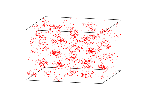
Figure 3: Modulated phase due to a Kirkwood instability. Here the random shift distribution is flat within a sphere with radius $\displaystyle\lambda=2$.

II.6 Corrections beyond Mean-field: the role of high dimensionality.

We can consider corrections to the mean-field equation of state. As we shall see, for finite $\displaystyle\lambda$ they vanish with dimensionality as $\displaystyle\propto\lambda^{-d}$. In the Mayer expansion of the entropy, the dominant correction will come from diagrams with $\displaystyle m=n$, which are the ring diagrams:

$$S_{an,\lambda}=N\ln N-\int\text{d}\mathbf{x}\rho(\mathbf{x})\left[\ln\rho(\mathbf{x})-1\right]+\hskip 2.27626pt\pbox[c]{2cm}{\lx@xy@svg{\hbox{\raise 0.0pt\hbox{\kern 0.0pt\hbox{\ignorespaces\ignorespaces\ignorespaces\hbox{\vtop{\kern 0.0pt\offinterlineskip\halign{\entry@#!@&&\entry@@#!@\cr&\crcr}}}\ignorespaces{\hbox{\kern 0.0pt\raise 0.0pt\hbox{\hbox{\kern-3.8889pt\raise-2.5pt\hbox{$\displaystyle\textstyle{\otimes}$}}}}}\ignorespaces{\hbox{\kern 14.1111pt\raise 0.0pt\hbox{\hbox{\kern 0.0pt\raise-2.5pt\hbox{$\displaystyle\textstyle{\otimes}$}}}}}\ignorespaces\ignorespaces\ignorespaces{}{\hbox{\lx@xy@droprule}}\ignorespaces{}{\hbox{\lx@xy@droprule}}{\hbox{\lx@xy@droprule}}{\hbox{\kern 15.0pt\raise 0.0pt\hbox{\hbox{\kern 0.0pt\raise 0.0pt\hbox{\hbox{\kern 3.0pt\raise 0.0pt\hbox{$\displaystyle\textstyle{}$}}}}}}}\ignorespaces}}}}\ignorespaces}+\pbox[c]{2cm}{\lx@xy@svg{\hbox{\raise 0.0pt\hbox{\kern 3.8889pt\hbox{\ignorespaces\ignorespaces\ignorespaces\hbox{\vtop{\kern 0.0pt\offinterlineskip\halign{\entry@#!@&&\entry@@#!@\cr&\\&&\crcr}}}\ignorespaces{\hbox{\kern-3.0pt\raise 0.0pt\hbox{\hbox{\kern 0.0pt\raise 0.0pt\hbox{\hbox{\kern 3.0pt\raise 0.0pt\hbox{$\displaystyle\textstyle{}$}}}}}}}{\hbox{\kern 9.0pt\raise 0.0pt\hbox{\hbox{\kern-3.8889pt\raise-2.5pt\hbox{$\displaystyle\textstyle{\otimes}$}}}}}\ignorespaces{\hbox{\kern 14.1111pt\raise-12.0pt\hbox{\hbox{\kern 0.0pt\raise-2.5pt\hbox{$\displaystyle\textstyle{\otimes}$}}}}}\ignorespaces\ignorespaces{}\ignorespaces\ignorespaces{\hbox{\lx@xy@drawline@}}\ignorespaces{}\ignorespaces\ignorespaces{\hbox{\lx@xy@drawline@}}\ignorespaces{\hbox{\lx@xy@drawline@}}\ignorespaces{\hbox{\kern-3.8889pt\raise-12.0pt\hbox{\hbox{\kern 0.0pt\raise-2.5pt\hbox{$\displaystyle\textstyle{\otimes}$}}}}}\ignorespaces\ignorespaces{}\ignorespaces\ignorespaces{\hbox{\lx@xy@drawline@}}\ignorespaces{}\ignorespaces\ignorespaces{\hbox{\lx@xy@drawline@}}\ignorespaces{\hbox{\lx@xy@drawline@}}{\hbox{\kern 0.0pt\raise-12.0pt\hbox{\hbox{\kern-3.8889pt\raise-2.5pt\hbox{$\displaystyle\textstyle{\otimes}$}}}}}\ignorespaces{\hbox{\kern 14.1111pt\raise-12.0pt\hbox{\hbox{\kern 0.0pt\raise-2.5pt\hbox{$\displaystyle\textstyle{\otimes}$}}}}}\ignorespaces\ignorespaces\ignorespaces{}{\hbox{\lx@xy@droprule}}\ignorespaces{}{\hbox{\lx@xy@droprule}}{\hbox{\lx@xy@droprule}}{\hbox{\kern 6.0pt\raise-12.0pt\hbox{\hbox{\kern 0.0pt\raise 0.0pt\hbox{\hbox{\kern 3.0pt\raise 0.0pt\hbox{$\displaystyle\textstyle{}$}}}}}}}{\hbox{\kern 15.0pt\raise-12.0pt\hbox{\hbox{\kern 0.0pt\raise 0.0pt\hbox{\hbox{\kern 3.0pt\raise 0.0pt\hbox{$\displaystyle\textstyle{}$}}}}}}}\ignorespaces}}}}\ignorespaces}+\pbox[c]{2cm}{\lx@xy@svg{\hbox{\raise 0.0pt\hbox{\kern 3.8889pt\hbox{\ignorespaces\ignorespaces\ignorespaces\hbox{\vtop{\kern 0.0pt\offinterlineskip\halign{\entry@#!@&&\entry@@#!@\cr&\\&\crcr}}}\ignorespaces{\hbox{\kern 0.0pt\raise 0.0pt\hbox{\hbox{\kern-3.8889pt\raise-2.5pt\hbox{$\displaystyle\textstyle{\otimes}$}}}}}\ignorespaces{\hbox{\kern-3.8889pt\raise-18.0pt\hbox{\hbox{\kern 0.0pt\raise-2.5pt\hbox{$\displaystyle\textstyle{\otimes}$}}}}}\ignorespaces\ignorespaces\ignorespaces{}{\hbox{\lx@xy@droprule}}\ignorespaces{}{\hbox{\lx@xy@droprule}}{\hbox{\lx@xy@droprule}}\ignorespaces{\hbox{\kern 14.1111pt\raise 0.0pt\hbox{\hbox{\kern 0.0pt\raise-2.5pt\hbox{$\displaystyle\textstyle{\otimes}$}}}}}\ignorespaces\ignorespaces\ignorespaces{}{\hbox{\lx@xy@droprule}}\ignorespaces{}{\hbox{\lx@xy@droprule}}{\hbox{\lx@xy@droprule}}{\hbox{\kern 18.0pt\raise 0.0pt\hbox{\hbox{\kern-3.8889pt\raise-2.5pt\hbox{$\displaystyle\textstyle{\otimes}$}}}}}\ignorespaces{\hbox{\kern 14.1111pt\raise-18.0pt\hbox{\hbox{\kern 0.0pt\raise-2.5pt\hbox{$\displaystyle\textstyle{\otimes}$}}}}}\ignorespaces\ignorespaces\ignorespaces{}{\hbox{\lx@xy@droprule}}\ignorespaces{}{\hbox{\lx@xy@droprule}}{\hbox{\lx@xy@droprule}}{\hbox{\kern-3.8889pt\raise-18.0pt\hbox{\hbox{\kern 0.0pt\raise-2.5pt\hbox{$\displaystyle\textstyle{\otimes}$}}}}}\ignorespaces{\hbox{\kern 14.1111pt\raise-18.0pt\hbox{\hbox{\kern 0.0pt\raise-2.5pt\hbox{$\displaystyle\textstyle{\otimes}$}}}}}\ignorespaces\ignorespaces\ignorespaces{}{\hbox{\lx@xy@droprule}}\ignorespaces{}{\hbox{\lx@xy@droprule}}{\hbox{\lx@xy@droprule}}{\hbox{\kern 14.1111pt\raise-18.0pt\hbox{\hbox{\kern 0.0pt\raise-2.5pt\hbox{$\displaystyle\textstyle{\otimes}$}}}}}\ignorespaces}}}}\ignorespaces}+\pbox[c]{2cm}{\lx@xy@svg{\hbox{\raise 0.0pt\hbox{\kern 3.8889pt\hbox{\ignorespaces\ignorespaces\ignorespaces\hbox{\vtop{\kern 0.0pt\offinterlineskip\halign{\entry@#!@&&\entry@@#!@\cr&&&&\\&&&&\\&&&&\crcr}}}\ignorespaces{\hbox{\kern-3.0pt\raise 0.0pt\hbox{\hbox{\kern 0.0pt\raise 0.0pt\hbox{\hbox{\kern 3.0pt\raise 0.0pt\hbox{$\displaystyle\textstyle{}$}}}}}}}{\hbox{\kern 3.28886pt\raise 0.0pt\hbox{\hbox{\kern 0.0pt\raise 0.0pt\hbox{\hbox{\kern 3.0pt\raise 0.0pt\hbox{$\displaystyle\textstyle{}$}}}}}}}{\hbox{\kern 12.57773pt\raise 0.0pt\hbox{\hbox{\kern-3.8889pt\raise-2.5pt\hbox{$\displaystyle\textstyle{\otimes}$}}}}}\ignorespaces{\hbox{\kern-3.8889pt\raise-12.0pt\hbox{\hbox{\kern 0.0pt\raise-2.5pt\hbox{$\displaystyle\textstyle{\otimes}$}}}}}\ignorespaces\ignorespaces{}\ignorespaces\ignorespaces{\hbox{\lx@xy@drawline@}}\ignorespaces{}\ignorespaces\ignorespaces{\hbox{\lx@xy@drawline@}}\ignorespaces{\hbox{\lx@xy@drawline@}}\ignorespaces{\hbox{\kern 21.26656pt\raise-12.0pt\hbox{\hbox{\kern 0.0pt\raise-2.5pt\hbox{$\displaystyle\textstyle{\otimes}$}}}}}\ignorespaces\ignorespaces{}\ignorespaces\ignorespaces{\hbox{\lx@xy@drawline@}}\ignorespaces{}\ignorespaces\ignorespaces{\hbox{\lx@xy@drawline@}}\ignorespaces{\hbox{\lx@xy@drawline@}}{\hbox{\kern 15.8666pt\raise 0.0pt\hbox{\hbox{\kern 0.0pt\raise 0.0pt\hbox{\hbox{\kern 3.0pt\raise 0.0pt\hbox{$\displaystyle\textstyle{}$}}}}}}}{\hbox{\kern 22.15546pt\raise 0.0pt\hbox{\hbox{\kern 0.0pt\raise 0.0pt\hbox{\hbox{\kern 3.0pt\raise 0.0pt\hbox{$\displaystyle\textstyle{}$}}}}}}}{\hbox{\kern 0.0pt\raise-12.0pt\hbox{\hbox{\kern-3.8889pt\raise-2.5pt\hbox{$\displaystyle\textstyle{\otimes}$}}}}}\ignorespaces{\hbox{\kern 2.39996pt\raise-24.33333pt\hbox{\hbox{\kern 0.0pt\raise-2.5pt\hbox{$\displaystyle\textstyle{\otimes}$}}}}}\ignorespaces\ignorespaces{}\ignorespaces\ignorespaces{\hbox{\lx@xy@drawline@}}\ignorespaces{}\ignorespaces\ignorespaces{\hbox{\lx@xy@drawline@}}\ignorespaces{\hbox{\lx@xy@drawline@}}{\hbox{\kern 3.28886pt\raise-12.0pt\hbox{\hbox{\kern 0.0pt\raise 0.0pt\hbox{\hbox{\kern 3.0pt\raise 0.0pt\hbox{$\displaystyle\textstyle{}$}}}}}}}{\hbox{\kern 9.57773pt\raise-12.0pt\hbox{\hbox{\kern 0.0pt\raise 0.0pt\hbox{\hbox{\kern 3.0pt\raise 0.0pt\hbox{$\displaystyle\textstyle{}$}}}}}}}{\hbox{\kern 15.8666pt\raise-12.0pt\hbox{\hbox{\kern 0.0pt\raise 0.0pt\hbox{\hbox{\kern 3.0pt\raise 0.0pt\hbox{$\displaystyle\textstyle{}$}}}}}}}{\hbox{\kern 25.15546pt\raise-12.0pt\hbox{\hbox{\kern-3.8889pt\raise-2.5pt\hbox{$\displaystyle\textstyle{\otimes}$}}}}}\ignorespaces{\hbox{\kern 14.97769pt\raise-24.33333pt\hbox{\hbox{\kern 0.0pt\raise-2.5pt\hbox{$\displaystyle\textstyle{\otimes}$}}}}}\ignorespaces\ignorespaces{}\ignorespaces\ignorespaces{\hbox{\lx@xy@drawline@}}\ignorespaces{}\ignorespaces\ignorespaces{\hbox{\lx@xy@drawline@}}\ignorespaces{\hbox{\lx@xy@drawline@}}{\hbox{\kern-3.0pt\raise-24.33333pt\hbox{\hbox{\kern 0.0pt\raise 0.0pt\hbox{\hbox{\kern 3.0pt\raise 0.0pt\hbox{$\displaystyle\textstyle{}$}}}}}}}{\hbox{\kern 2.39996pt\raise-24.33333pt\hbox{\hbox{\kern 0.0pt\raise-2.5pt\hbox{$\displaystyle\textstyle{\otimes}$}}}}}\ignorespaces{\hbox{\kern 14.97769pt\raise-24.33333pt\hbox{\hbox{\kern 0.0pt\raise-2.5pt\hbox{$\displaystyle\textstyle{\otimes}$}}}}}\ignorespaces\ignorespaces\ignorespaces{}{\hbox{\lx@xy@droprule}}\ignorespaces{}{\hbox{\lx@xy@droprule}}{\hbox{\lx@xy@droprule}}{\hbox{\kern 9.57773pt\raise-24.33333pt\hbox{\hbox{\kern 0.0pt\raise 0.0pt\hbox{\hbox{\kern 3.0pt\raise 0.0pt\hbox{$\displaystyle\textstyle{}$}}}}}}}{\hbox{\kern 14.97769pt\raise-24.33333pt\hbox{\hbox{\kern 0.0pt\raise-2.5pt\hbox{$\displaystyle\textstyle{\otimes}$}}}}}{\hbox{\kern 22.15546pt\raise-24.33333pt\hbox{\hbox{\kern 0.0pt\raise 0.0pt\hbox{\hbox{\kern 3.0pt\raise 0.0pt\hbox{$\displaystyle\textstyle{}$}}}}}}}\ignorespaces}}}}\ignorespaces}+\dots \textstyle{\otimes} \textstyle{\otimes} \textstyle{\otimes} \textstyle{\otimes} \textstyle{\otimes} \textstyle{\otimes} \textstyle{\otimes} \textstyle{\otimes} \textstyle{\otimes} \textstyle{\otimes} \textstyle{\otimes} \textstyle{\otimes} \textstyle{\otimes} \textstyle{\otimes} \textstyle{\otimes} \textstyle{\otimes} \textstyle{\otimes} \textstyle{\otimes} \textstyle{\otimes} \textstyle{\otimes} \textstyle{\otimes} \textstyle{\otimes} \textstyle{\otimes} \textstyle{\otimes} \textstyle{\otimes} \textstyle{\otimes} \textstyle{\otimes} \textstyle{\otimes} \textstyle{\otimes} \textstyle{\otimes} \textstyle{\otimes} \textstyle{\otimes} \textstyle{\otimes} \textstyle{\otimes} \textstyle{\otimes} \textstyle{\otimes} \textstyle{\otimes} \textstyle{\otimes} \textstyle{\otimes} \textstyle{\otimes} \textstyle{\otimes} \textstyle{\otimes} \textstyle{\otimes} \textstyle{\otimes} \textstyle{\otimes} \textstyle{\otimes} \textstyle{\otimes} \textstyle{\otimes} \textstyle{\otimes} \textstyle{\otimes}$$ (34)

The resummation of these diagrams has been done by Montroll and Mayer mayer1941statistical :

$$\frac{S_{an,\lambda}}{N}=1-\ln\rho-\frac{1}{2}\rho v_{d}+\frac{1}{2}\frac{1}{(2\pi)^{d}}\rho^{2}\int\Omega_{d}k^{d-1}\text{d}k\frac{\left[\tilde{f}(k)\right]^{3}}{1-\rho\tilde{f}(k)}+\ln N$$ (35)

and gives, for $\displaystyle\lambda\gg 1$:

$$\begin{array}[]{rl}\frac{S_{an,\lambda}}{N}&=1-\ln\rho-\frac{1}{2}\rho v_{d}-\frac{1}{2}\frac{1}{(2\pi)^{d}}\rho^{2}\int\Omega_{d}k^{d-1}\text{d}k\frac{\left[v_{d}\tilde{P}_{\lambda}(k)\right]^{3}}{1+\rho v_{d}\tilde{P}_{\lambda}(k)}+\ln N\\ &=1-\ln\rho-\frac{1}{2}\rho v_{d}-\frac{1}{2}\frac{1}{(2\pi)^{d}\lambda^{d}}\rho^{2}I_{31}(\rho)+\ln N\end{array}$$ (36)

where we have introduced the $\displaystyle\lambda$-independent factor:

$$I_{ab}(\rho)=\int\Omega_{d}k^{d-1}\text{d}k\frac{\left[v_{d}\tilde{P}_{1}(k)\right]^{a}}{\left[1+\rho v_{d}\tilde{P}_{1}(k)\right]^{b}}$$ (37)

The equation of state is then:

$$P=\rho+\frac{1}{2}\rho^{2}v_{d}+\frac{\rho^{3}}{(2\pi)^{d}\lambda^{d}}\left[I_{31}(\rho)-\frac{\rho}{2}I_{42}(\rho)\right]$$ (38)

This expression gives a quantitative estimation of how the approximation becomes better at higher dimensions, through the factor $\displaystyle\lambda^{d}$. Already in $\displaystyle d=3$, the ring corrections are less than 1% at $\displaystyle\phi=1$ for a range as small f as $\displaystyle\lambda=1$. When $\displaystyle d>3$, one needs to take a very small range of random shifts to feel any finite dimensional effect.

II.7 Estimation of the density as $\displaystyle P\rightarrow\infty$

The model with $\displaystyle\lambda\rightarrow\infty$ has a maximal packing density that diverges in the thermodynamic limit, a rather awkward property from the thermodynamic point of view. When $\displaystyle\lambda\to\infty$ we can derive an estimation of the maximum density of the random shift model. To do this, we consider the following algorithm:

i) Starting a configuration with $\displaystyle N$ spheres in a volume $\displaystyle V$, generate $\displaystyle N$ random shifts,

ii) Locate positions where one can add, without any overlap, a new sphere interacting with other spheres via the $\displaystyle N$ random shifts,

iii) If such a position exists, add this $\displaystyle(N+1)$th sphere, and go back to step $\displaystyle 1$.

Up to which density such an algorithm can work? When $\displaystyle\lambda\to\infty$, the $\displaystyle(N+1)$th sphere will see the other spheres as having completely random positions. Then the probability for a position $\displaystyle\mathbf{x}$ to satisfy the hard sphere constraints imposed by the $\displaystyle N$ other spheres is simply:

$$P_{N}(\mathbf{x})=\left(1-\frac{v_{d}}{V}\right)^{N}\simeq e^{-\frac{Nv_{d}}{V}}=e^{-\phi}$$ (39)

Then the available volume to place the $\displaystyle(N+1)$th sphere will be $\displaystyle Ve^{-\phi}$. The algorithm will not be able to find a solution once the available volume is of the order of $\displaystyle v_{d}$. If we note $\displaystyle\phi_{max}$ the volume fraction for which this happens, we have:

$$e^{-\phi_{max}}\sim\frac{v_{d}}{V}$$ (40)

which gives:

$$\phi_{max}\sim\ln\frac{V}{v_{d}}=\ln N-\ln(\ln N)+\ln(\ln(\ln N))...$$ (41)

We implemented this algorithm for the random shift model in $\displaystyle d=1$. Results are presented in Fig. 4, showing the $\displaystyle\ln N$ dependence of $\displaystyle\phi_{max}$.

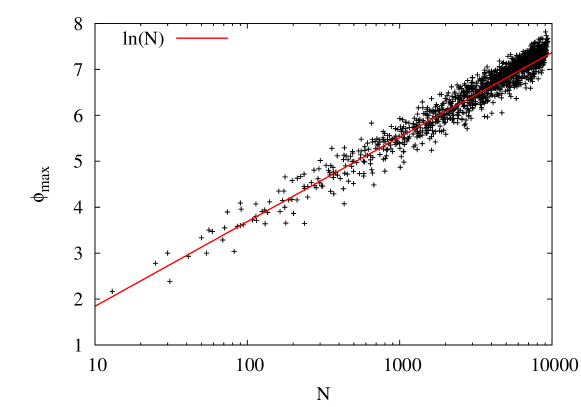
Figure 4: Maximum density $\displaystyle\phi_{max}$ obtained by the algorithm described in the main text, showing the $\displaystyle\ln N$ dependence of Eq. (41).

III Dynamics in the liquid phase

III.1 A warming up exercise: computation of the canonical partition function

The essential steps followed to compute the exact dynamic equation are similar to the ones performed in making an equilibrium computation in the canonical ensemble. It is thus instructive to understand them in this context first. Starting again from Eq. (11), and introducing the density $\displaystyle\rho(\underline{\mathbf{x}})$ by:

$$\rho(\mathbf{x})=\sum_{i}\delta(\mathbf{x}-\mathbf{x_{i}})$$ (42)

with $\displaystyle{\bf x_{i}}$ the coordinate of the $\displaystyle i-th$ particle, we can rewrite $\displaystyle\overline{Z_{\{\mathbf{A}\}}}$ as:

$$\overline{Z_{\{\mathbf{A}\}}}=\int\text{d}\mathbf{x_{i}}\int\mathscr{D}[\rho(\mathbf{x})]\delta\left(\rho(\mathbf{x})-\sum_{i}\delta(\mathbf{x}-\mathbf{x}_{i})\right)\exp\left[\frac{1}{2}\int\text{d}\mathbf{x}\text{d}\mathbf{y}\rho(\mathbf{x})\rho(\mathbf{y})\ln\left[1+\overline{f}(\mathbf{x_{i}}-\mathbf{x_{j}})\right]\right]$$ (43)

Now we can exponentiate the $\displaystyle\delta$ constraint using a second field $\displaystyle\hat{\rho}$, and integrate over the $\displaystyle\underline{\mathbf{x_{i}}}$’s:

$$\begin{array}[]{rl}\overline{Z_{\{\mathbf{A}\}}}=\int&\mathscr{D}[\rho(\mathbf{x})]\mathscr{D}[\hat{\rho}(\mathbf{x})]\\ &\exp\left\{i\int\text{d}\mathbf{x}\hat{\rho}(\mathbf{x})\rho(\mathbf{x})+N\ln\int\text{d}\mathbf{x}e^{-i\hat{\rho}(\mathbf{x})}+\frac{1}{2}\int\text{d}\mathbf{x}\text{d}\mathbf{y}\rho(\mathbf{x})\rho(\mathbf{y})\ln\left[1+\overline{f}(\mathbf{x_{i}}-\mathbf{x_{j}})\right]\right\}\end{array}$$ (44)

Again noticing that:

$$\overline{f}(\mathbf{x}-\mathbf{y})=-\frac{v_{d}}{V}$$ (45)

we can expand the logarithm to get:

$$\begin{array}[]{rl}\overline{Z_{\{\mathbf{A}\}}}=\int&\mathscr{D}[\rho(\mathbf{x})]\mathscr{D}[\hat{\rho}(\mathbf{x})]\\ &\exp\left\{i\int\text{d}\mathbf{x}\hat{\rho}(\mathbf{x})\rho(\mathbf{x})+N\ln\int\text{d}\mathbf{x}e^{-i\hat{\rho}(\mathbf{x})}+\frac{1}{2}\int\text{d}\mathbf{x}\text{d}\mathbf{y}\rho(\mathbf{x})\rho(\mathbf{y})\overline{f}(\mathbf{x}-\mathbf{y})\right\}\end{array}$$ (46)

This integral may be evaluated by saddle point with respect to the fields $\displaystyle\rho$ and $\displaystyle\hat{\rho}$ (note that each term in the exponential is of order $\displaystyle N$, including the last one, due to the value of $\displaystyle\overline{f}$). This gives:

$$\begin{array}[]{rl}\rho(\mathbf{x})&=N\frac{e^{-i\hat{\rho}(\mathbf{x})}}{\int\text{d}\mathbf{x}e^{-i\hat{\rho}(\mathbf{x})}}\\ \hat{\rho}(\mathbf{x})&=i\int\text{d}\mathbf{y}\rho(\mathbf{y})\overline{f}(\mathbf{x}-\mathbf{y})\end{array}$$ (47)

Thus, the logarithm of the partition function can be written in terms of $\displaystyle\rho$ as:

$$\ln\overline{Z_{\{\mathbf{A}\}}}=-\int\text{d}\mathbf{x}\rho(\mathbf{x})\ln\rho(\mathbf{x})+\frac{1}{2}\int\text{d}\mathbf{x}\text{d}\mathbf{y}\rho(\mathbf{x})\rho(\mathbf{y})\overline{f}(\mathbf{x}-\mathbf{y})+N\ln N$$ (48)

Below, we shall follow the same steps, but with trajectories playing the role of particles.

III.2 Derivation of the exact dynamics as a partition function of trajectories

We wish to study the dynamics of the model in the mean-field limit, starting from the Langevin equation:

$$\dot{\mathbf{x}}_{i}(t)=-\sum_{j\neq i}\nabla_{i}V(\mathbf{x}_{i}(t)-\mathbf{x}_{j}(t)-\mathbf{A}_{ij})+\bm{\eta}_{i}(t)+\mathbf{h}_{i}(t),$$ (49)

where we have introduced an external field $\displaystyle\mathbf{h}_{i}(t)$, which acts as a source term, and will later be set to zero. The vector $\displaystyle\bm{\eta}_{i}(t)$ is a Gaussian white noise with variance $\displaystyle 2T$, where $\displaystyle T$ is the temperature, that we will keep explicit for all the derivation of the dynamics equations:

$$<\bm{\eta}_{i}(t)\bm{\eta}_{j}(t^{\prime})>=2Td\;\delta_{ij}\;\delta(t-t^{\prime})$$ (50)

We denote $\displaystyle P(\{\mathbf{x}^{0}\},\{\mathbf{x}^{\tau}\},\tau)$ the probability of having particle $\displaystyle i$ in $\displaystyle\mathbf{x}^{0}_{i}$ at time $\displaystyle t=0$ and in $\displaystyle\mathbf{x}^{\tau}_{1}$ at time $\displaystyle t=\tau$, in the absence of external field $\displaystyle\mathbf{h}$. We may express this as a sum over paths using the Martin-Siggia-Rose/ DeDominicis-Jensen zinn2002quantum formalism. Averaging over the noise, this gives:

$$\displaystyle P(\{\mathbf{x}^{0}\},\{\mathbf{x}^{\tau}\},\tau) \displaystyle= \displaystyle\int\prod_{ij}\text{d}\mathbf{A}_{ij}P(\mathbf{A}_{ij})$$ (51)

$$\displaystyle\quad\int_{\{\mathbf{x}(0)\}=\{\mathbf{x}^{0}\}}^{\{\mathbf{x}(\tau)\}=\{\mathbf{x}^{\tau}\}}\prod_{i}\text{D}[\mathbf{x}_{i}(t),\hat{\mathbf{x}}_{i}(t)]\exp\left[-\mathcal{S}[\{\mathbf{x}_{i}(t)\},\{\hat{\mathbf{x}}_{i}(t)\}]\right],$$

with

$$\begin{array}[]{rl}\mathcal{S}[\{\mathbf{x}_{i}(t)\},\{\hat{\mathbf{x}}_{i}(t)\}]&=\int_{0}^{\tau}\mbox{d}t\left[\sum_{i}\left(\dot{\mathbf{x}}_{i}(t)\hat{\mathbf{x}}_{i}(t)+\hat{\mathbf{x}}_{i}(t)\hat{\mathbf{x}}_{i}(t)\right)\right]\\ &\;\;\;+\int_{0}^{\tau}\mbox{d}t\left[\frac{1}{2}\sum_{<ij>}\left(\hat{\mathbf{x}}_{i}(t)\nabla_{i}V(\mathbf{x}_{i}-\mathbf{x}_{j}-\mathbf{A}_{ij}))+\hat{\mathbf{x}}_{j}(t)\nabla_{j}V(\mathbf{x}_{j}-\mathbf{x}_{i}-\mathbf{A}_{ji})\right)\right]\\ &=\sum_{i}\Phi[\mathbf{x}_{i}(t),\hat{\mathbf{x}}_{i}(t)]+\sum_{ij}W_{ij}[\mathbf{x}_{i}(t),\hat{\mathbf{x}}_{i}(t),\mathbf{x}_{j}(t),\hat{\mathbf{x}}_{j}(t)]\end{array}$$ (52)

where the last two lines define $\displaystyle\Phi$ and $\displaystyle W_{ij}$. Integrations in Eq. (51) of the variables $\displaystyle\hat{\mathbf{x}}_{i}(t)$ are along the imaginary axis. The quantity $\displaystyle P[\{\mathbf{x}_{i}(t)\},\{\hat{\mathbf{x}}_{i}(t)\}]=\exp\left[-\mathcal{S}[\{\mathbf{x}_{i}(t)\},\{\hat{\mathbf{x}}_{i}(t)\}]\right]$ may seem mysterious, because of the variables $\displaystyle\hat{\mathbf{x}}_{i}(t)$, which do not have an immediate physical meaning. In order to understand them, we consider the probability of paths in the presence of external fields $\displaystyle\{\mathbf{h}_{i}(t)\}$:

$$P[\{\mathbf{x}_{i}(t)\},\{\hat{\mathbf{x}}_{i}(t)\},\{\mathbf{h}_{i}(t)\}]=\exp\left\{-\mathcal{S}[\{\mathbf{x}_{i}(t)\},\{\hat{\mathbf{x}}_{i}(t)\}]-\hat{\mathbf{x}}_{i}(t)\mathbf{h}_{i}(t)\right\},$$ (53)

Integrating over the ‘hat’ variables, we find that:

$$\begin{array}[]{rl}P[\{\mathbf{x}_{i}(t)\},\{\mathbf{h}_{i}(t)\}]&=\int\prod_{i}\text{D}[\hat{\mathbf{x}}_{i}(t)]P[\{\mathbf{x}_{i}(t)\},\{\hat{\mathbf{x}}_{i}(t)\},\{\mathbf{h}_{i}(t)\}]\\ &=\int\prod_{i}\text{D}[\hat{\mathbf{x}}_{i}(t)]e^{\hat{\mathbf{x}}_{i}(t)\mathbf{h}_{i}(t)}P[\{\mathbf{x}_{i}(t)\},\{\hat{\mathbf{x}}_{i}(t)\}]\end{array}$$ (54)

In other words, the ‘hat’ variables $\displaystyle\{\hat{\mathbf{x}}_{i}(t)\}$ are the Fourier-transform variables of the fields: the probability of a trajectory $\displaystyle(\{\mathbf{x}_{i}(t)\},\{\hat{\mathbf{x}}_{i}(t)\})$ in the absence of field, is the Fourier transform of the corresponding physical probability $\displaystyle\{\mathbf{x}_{i}(t)\}$ in the presence of an external field $\displaystyle\{\mathbf{h}_{i}(t)\}$.

The functional formalism casts the dynamical problem into a form that resembles a partition function, but with one-dimensional objects (the trajectories) replacing the point particles. We may exploit the analogy to repeat the canonical computation in the preceding subsection. In particular, we may define the ‘dynamical Mayer function’ as:

$$1+\overline{f}_{d}[\mathbf{x}_{i}(t),\hat{\mathbf{x}}_{i}(t),\mathbf{x}_{j}(t),\hat{\mathbf{x}}_{j}(t)]=\int\text{d}\mathbf{A}_{ij}P(\mathbf{A}_{ij})\exp\left\{-W_{ij}[\mathbf{x}_{i}(t),\hat{\mathbf{x}}_{i}(t),\mathbf{x}_{j}(t),\hat{\mathbf{x}}_{j}(t)]\right\}$$ (55)

and introduce the dynamical ‘partition function’:

$$\begin{array}[]{rl}\overline{Z_{N,\tau}}&=\int\prod_{i}\text{d}\mathbf{x}^{0}_{i}\text{d}\mathbf{x}^{\tau}_{i}P_{\{\mathbf{A}\}}(\{\mathbf{x}^{0}\},\{\mathbf{x}^{\tau}\},\tau)\\ &=\int\prod_{i}\left(\text{D}[\mathbf{x}_{i}(t),\hat{\mathbf{x}}_{i}(t)]e^{-\Phi[\mathbf{x}_{i}(t),\hat{\mathbf{x}}_{i}(t)]}\right)\prod_{ij}\left(1+\overline{f}_{d}[\mathbf{x}_{i}(t),\hat{\mathbf{x}}_{i}(t),\mathbf{x}_{j}(t),\hat{\mathbf{x}}_{j}(t)]\right)\end{array}$$ (56)

In the above expression the path integral is now performed over paths with free boundary conditions. The initial conditions are weighted with a flat distribution. With these small reinterpretations, $\displaystyle\overline{Z_{N,\tau}}$ looks like the (static) partition function of $\displaystyle N$ ’polymers’ $\displaystyle(\mathbf{x}(t),\hat{\mathbf{x}}(t))$, in an external field $\displaystyle\Phi$, interacting via a potential $\displaystyle\ln\left[1+\overline{f}_{d}\right]$.

Next we introduce a density field:

$$\rho[\mathbf{x}(t),\hat{\mathbf{x}}(t)]=\sum_{i}\delta[\mathbf{x}(t)-\mathbf{x}_{i}(t)]\delta[\hat{\mathbf{x}}(t)-\hat{\mathbf{x}}_{i}(t)]$$ (57)

Note that $\displaystyle\delta$ is here a Dirac function in the sense of trajectories, i.e. a product of ordinary deltas, one for each time. Inserting this field in the partition function we obtain:

$$\prod_{i}e^{-\Phi[\mathbf{x}_{i}(t),\hat{\mathbf{x}}_{i}(t)]}=\exp\left[-\int\text{D}[\mathbf{x}(t),\hat{\mathbf{x}}(t)]\rho[\mathbf{x}(t),\hat{\mathbf{x}}(t)]\Phi[\mathbf{x}(t),\hat{\mathbf{x}}(t)]\right],$$ (58)

and:

$$\begin{array}[]{rl}\prod_{i\neq j}\left(1+\overline{f}_{d}[\mathbf{x}_{i}(t),\hat{\mathbf{x}}_{i}(t),\mathbf{x}_{j}(t),\hat{\mathbf{x}}_{j}(t)]\right)&=\exp\bigg{[}\frac{1}{2}\int\text{D}[\mathbf{x}(t),\hat{\mathbf{x}}(t)]\text{D}[\mathbf{y}(t),\hat{\mathbf{y}}(t)]\\ &\rho[\mathbf{x}(t),\hat{\mathbf{x}}(t)]\rho[\mathbf{y}(t),\hat{\mathbf{y}}(t)]\ln\left(1+\overline{f}_{d}[\mathbf{x}(t),\hat{\mathbf{x}}(t),\mathbf{y}(t),\hat{\mathbf{y}}(t)]\right)\bigg{]}.\end{array}$$ (59)

Note that the right-hand side contains a self-interaction term that was not present on the left-hand side, but this term is negligible compared to the interparticle interactions.

As in the static case, looking more closely to the function $\displaystyle\overline{f}_{d}$ defined by Eq. (55), we see that in the integral over disorder, the integrand is $\displaystyle 1$ if the two trajectories do not interact. These trajectories do interact if the random shift is able to bring them close to one another. If the trajectories explore a finite volume during between times $\displaystyle 0$ and $\displaystyle\tau$ (ie $\displaystyle\tau$ is not too large, at least much smaller than the ergodic time), this is only possible for a finite volume of integration on the random shift. As the distribution of the shifts is $\displaystyle P(\mathbf{A})=1/V$, this means that the function $\displaystyle\overline{f}_{d}$ is of order $\displaystyle\Gamma/V$, where $\displaystyle\Gamma$ is the typical volume covered by a trajectory during an time interval $\displaystyle\tau$. Then, just as in the static calculation, we may use that $\displaystyle\ln(1+\overline{f}_{d})\simeq\overline{f}_{d}$. Now, imposing the condition Eq. (57) via:

$$\begin{array}[]{rl}&\delta\bigg{[}\rho[\mathbf{x}(t),\hat{\mathbf{x}}(t)]-\sum_{i}\delta[\mathbf{x}(t)-\mathbf{x}_{i}(t)]\delta[\hat{\mathbf{x}}(t)-\hat{\mathbf{x}}_{i}(t)]\bigg{]}=\int D\left[\hat{\rho}[\mathbf{x}(t),\hat{\mathbf{x}}(t)]\right]\\ &\qquad\qquad e^{i\int\text{D}[\mathbf{x}(t),\hat{\mathbf{x}}(t)]\rho[\mathbf{x}(t),\hat{\mathbf{x}}(t)]\hat{\rho}[\mathbf{x}(t),\hat{\mathbf{x}}(t)]-i\hat{\rho}[\mathbf{x}(t),\hat{\mathbf{x}}(t)]\sum_{i}\delta[\mathbf{x}(t)-\mathbf{x}_{i}(t)]\delta[\hat{\mathbf{x}}(t)-\hat{\mathbf{x}}_{i}(t)]}\end{array}$$ (60)

and integrating over $\displaystyle\mathbf{x}_{i}(t)$’s and $\displaystyle\hat{\mathbf{x}}_{i}(t)$’s, we get, for a system at equilibrium at time $\displaystyle 0$ (we dropped the time dependence of the paths to simplify the notation):

$$\begin{array}[]{rl}Z_{N,\tau}&=\int D[\rho]D[\hat{\rho}]\exp\bigg{\{}i\int\text{D}[\mathbf{x},\hat{\mathbf{x}}]\rho[\mathbf{x},\hat{\mathbf{x}}]\hat{\rho}[\mathbf{x},\hat{\mathbf{x}}]+N\ln\int\text{D}[\mathbf{x},\hat{\mathbf{x}}]e^{-i\hat{\rho}[\mathbf{x},\hat{\mathbf{x}}]}\\ &-\int\text{D}[\mathbf{x},\hat{\mathbf{x}}]\rho[\mathbf{x},\hat{\mathbf{x}}]\Phi[\mathbf{x},\hat{\mathbf{x}}]+\frac{1}{2}\int\text{D}[\mathbf{x},\hat{\mathbf{x}}]\text{D}[\mathbf{y},\hat{\mathbf{y}}]\rho[\mathbf{x},\hat{\mathbf{x}}]\rho[\mathbf{y},\hat{\mathbf{y}}]\overline{f}_{d}[\mathbf{x},\hat{\mathbf{x}},\mathbf{y},\hat{\mathbf{x}}]\bigg{\}}\end{array}$$ (61)

For the mean-field dynamics we can take the saddle-point with respect to $\displaystyle\rho$ and $\displaystyle\hat{\rho}$ of the last equation. This reads:

$$\begin{array}[]{rl}\rho[\mathbf{x},\hat{\mathbf{x}}]&=N\frac{e^{-i\hat{\rho}[\mathbf{x},\hat{\mathbf{x}}]}}{\int\text{D}[\mathbf{x},\hat{\mathbf{x}}]e^{-i\hat{\rho}[\mathbf{x},\hat{\mathbf{x}}]}},\\ \hat{\rho}[\mathbf{x},\hat{\mathbf{x}}]&=-i\Phi[\mathbf{x},\hat{\mathbf{x}}]+i\int\text{D}[\mathbf{y},\hat{\mathbf{y}}]\rho[\mathbf{y},\hat{\mathbf{y}}]\overline{f}_{d}[\mathbf{x},\hat{\mathbf{x}},\mathbf{y},\hat{\mathbf{y}}].\end{array}$$ (62)

which gives a closed equation on the density of paths $\displaystyle\rho[\mathbf{x},\hat{\mathbf{x}}]$:

$$\rho[\mathbf{x},\hat{\mathbf{x}}]=\frac{1}{\mathcal{N}}e^{-\Phi[\mathbf{x},\hat{\mathbf{x}}]+\int\text{D}[\mathbf{y},\hat{\mathbf{y}}]\rho[\mathbf{y},\hat{\mathbf{y}}]\overline{f}_{d}[\mathbf{x},\hat{\mathbf{x}},\mathbf{y},\hat{\mathbf{y}}]}$$ (63)

where $\displaystyle\mathcal{N}$ ensures that the density is normalized to $\displaystyle N$.

Reinserting this equation in the partition function, we get the functional $\displaystyle\mathcal{S}=-\ln Z$, which reads:

$$\begin{array}[]{rl}\mathcal{S}[\rho]&=\int\text{D}[\mathbf{x},\hat{\mathbf{x}}]\rho[\mathbf{x},\hat{\mathbf{x}}]\ln\left[\rho[\mathbf{x},\hat{\mathbf{x}}]\right]+\int\text{D}[\mathbf{x},\hat{\mathbf{x}}]\rho[\mathbf{x},\hat{\mathbf{x}}]\Phi[\mathbf{x},\hat{\mathbf{x}}]+\mathcal{S}_{int}[\rho]-N\ln N\\ &\mathcal{S}_{int}[\rho]=-\frac{1}{2}\int\text{D}[\mathbf{x},\hat{\mathbf{x}}]\text{D}[\mathbf{y},\hat{\mathbf{y}}]\rho[\mathbf{x},\hat{\mathbf{x}}]\rho[\mathbf{y},\hat{\mathbf{y}}]\overline{f}_{d}[\mathbf{x},\hat{\mathbf{x}},\mathbf{y},\hat{\mathbf{y}}]\end{array}$$ (64)

Eq. (63) is the counterpart of the saddle point equation (47) obtained in the previous subsection for the average density. As happens often in this kind of problems, even the mean-field equations are hard to solve, in this case because the complexity of an object like $\displaystyle\rho[\mathbf{x},\hat{\mathbf{x}}]$ makes the problem intractable. But, just as in equilibrium calculations, we can try, as a further approximation, to find extrema of the free energy Eq. (63) in a well chosen restricted subspace of all possible $\displaystyle\rho[\mathbf{x},\hat{\mathbf{x}}]$. The next subsection is devoted to the search of such an ansatz.

III.3 An approximation in terms of two-point functions

In terms of physical quantities, the simplest trial form for the probabilities is to propose a Gaussian form:

$$\displaystyle\ln P[\{\mathbf{x}(t)\},\{\mathbf{h}(t)\}]=$$

$$\displaystyle\;\;\;\;\;\;-\frac{1}{2}\int\text{d}t_{a}\;\text{d}t_{b}\;\{A_{1}(t_{a},t_{b}){\bf h}(t_{a}){\bf h}(t_{b})+A_{2}(t_{a},t_{b}){\bf h}(t_{a}){\bf x}(t_{b})+A_{3}(t_{a},t_{b}){\bf x}(t_{a}){\bf x}(t_{b})\}$$ (65)

This leads, equivalently, to proposing an ansatz that is Gaussian in the $\displaystyle\{{\bf x,{\hat{x}}}\}$ variables. This ansatz has to be invariant with respect to a time-independent translation of the trajectory, which may be imposed, in terms of the $\displaystyle{\bf x,{\hat{x}}}$ variables, by the form:

$$\begin{array}[]{rl}&P[\{\mathbf{x}(t)\},\{{\bf{\hat{x}}(t)}\}]=\int\text{d}{\bf\bar{x}}\;\;\exp\bigg{[}-\frac{1}{2}\int\text{d}t_{a}\;\text{d}t_{b}\;\{{\tilde{B}}(t_{a},t_{b}){\bf{\hat{x}}}(t_{a}){\bf{\hat{x}}}(t_{b})\\ &\;\;\;\;\;\;\;+{\tilde{R}}(t_{b},t_{a}){\bf{\hat{x}}}(t_{b})({\bf x}(t_{a})-{\bf\bar{x}})+{\tilde{R}}(t_{a},t_{b}){\bf{\hat{x}}}(t_{a})({\bf x}(t_{b})-{\bf\bar{x}})+{\tilde{D}}(t_{a},t_{b})({\bf x}(t_{a})-{\bf\bar{x}})({\bf x}(t_{b})-{\bf\bar{x})}\}\bigg{]}\end{array}$$ (66)

where the integration over $\displaystyle{\bf\bar{x}}$ is over the whole volume and implements the translational invariance of the ansatz, i.e. that the quadratic form has a zero-mode in the translations. (A similar strategy has been previously used in a static replica ansatz, and it is the same idea as the Hill-Wheeler integral that imposes rotational invariance in nuclear theory). It will turn out that, in equilibrium, the ansatz satisfies the causality and fluctuation-dissipation relations :

$$\begin{array}[]{rl}{\tilde{D}}(t,t^{\prime})&=0\\ {\tilde{R}(t,t^{\prime})}&=-\frac{1}{T}\frac{\partial}{\partial t}{\tilde{B}}(t-t^{\prime})\Theta(t-t^{\prime})\end{array}$$ (67)

The calculation is cumbersome, and we leave it for Appendix B. The result is expressed in terms of the two-time correlation function:

$$B(t-t^{\prime})=\frac{1}{N}\sum_{a}\;\langle({\bf x}_{a}(t)-{\bf x}_{a}(t^{\prime}))^{2}\rangle$$ (68)

where the average is over the Langevin noise and the initial conditions. It may be written in the (superficially) Mode-Coupling-like format:

$$\frac{\partial B(t)}{\partial t_{a}}=\int\text{d}t^{\prime}\Sigma_{R}[B](t-t^{\prime})B(t^{\prime})+2T$$ (69)

with $\displaystyle t>0$. This form is quite general, what defines our equation is the kernel $\displaystyle\Sigma_{R}$, which in Mode-Coupling equations is a simple function of $\displaystyle B$, and here is computed as follows. Define first the response function $\displaystyle R(t)$, which satisfies the Fluctuation-dissipation theorem:

$$R(t)=-\frac{1}{T}\frac{\partial B(t)}{\partial t}\Theta(-t)$$ (70)

Then the kernel is:

$$\Sigma_{R}(t_{a}-t_{b})=\frac{2}{T}\int\text{d}t_{a^{\prime}}\text{d}t_{b^{\prime}}\;{R}^{-1}(t_{a}-t_{a^{\prime}})\;\frac{\partial}{\partial t_{a^{\prime}}}\langle\mathbf{x}(t_{a^{\prime}})\mathbf{x}(t_{b^{\prime}})\rangle_{int}\;{R}^{-1}(t_{b^{\prime}}-t_{b})$$ (71)

where $\displaystyle R^{-1}$ is the inverse through convolution of $\displaystyle R$:

$$\int\text{d}t^{\prime}\;R(t-t^{\prime})R^{-1}(t^{\prime})=\delta(t)$$ (72)

and may be obtained from $\displaystyle R$ easily with Laplace transforms. Self-consistency is imposed by the definition

$$\begin{array}[]{rl}{\tilde{R}}&=R^{-1}\\ {\tilde{B}}(t)&=\int\text{d}t"\text{d}t^{\prime}\;R^{-1}(t-t^{\prime\prime})B(t"-t^{\prime})R^{-1}(t^{\prime})\end{array}$$ (73)

The trajectories that contribute to the averages $\displaystyle\langle\bullet\rangle_{int}$ are those in which two particles enter at any intermediate time within the interaction range, as depicted in figure 5, otherwise their contribution vanishes, as in a static Mayer expansion.

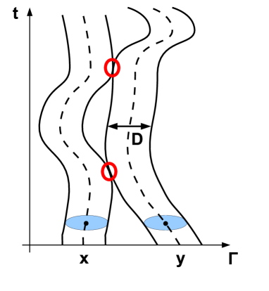
Figure 5: The trajectories contributing to a Mayer diagram are those that come into interaction range at some time.

IV Numerical results from $\displaystyle\lambda=\infty$ to $\displaystyle\lambda=0$

In order to investigate the system beyond mean-field, we studied the finite $\displaystyle\lambda$ case by numerical simulations. We used two different Monte-Carlo algorithms, an isobaric-isothermal one for the study of the equation of state, and an isovolumic-isothermal one for the study of the dynamics close to the glass transition. We worked with systems of $\displaystyle 864$ particles. The system we looked at for the bidisperse case is a 50:50 mixture of particles of diameter $\displaystyle 1$ and $\displaystyle 1.4$, a common choice for a three dimensional bidisperse glass former o2002random ; PhysRevLett.102.085703 .

We equilibrate the system at increasing pressures by annealing simulations. We check carefully that equilibrium is reached at every studied pressure by performing annealings with several compression rates, and ensuring that they give the same values for a given observable, e. g. density. Close to the glass transition, we also check that no aging is visible in the system.

IV.1 Simulations in the mean-field case

In the $\displaystyle\lambda\to\infty$ limit, equilibrating the system can be much easier, thanks to the ‘planting’ technique krzakala2009hiding ; achlioptas2008algorithmic : for mean-field problems with quenched random variables, if the annealed free energy is exact ($\displaystyle\overline{\ln Z}=\ln\overline{Z}$), one can create an instance in thermal equilibrium by taking a random set of variables (here particle positions), and looking for a disorder (here random shifts) compatible with this set, ie leading to $\displaystyle H(\{\mathbf{x}\},\{\mathbf{A}\})=0$. One can show that, within mean-field, this creates no bias in the measure. In our model, this means that we can generate safely an equilibrium instance as long as the annealed entropy Eq. (14) is valid, ie as long as the liquid is the equilibrium phase. Finding an equilibrium instance in this ensemble requires at most a few tens of seconds for a system with $\displaystyle 1000$ particles on a desktop computer. This of course, is very useful as we can get easily equilibrated configurations with densities close and even above the dynamic glass transition density, as long as we do not reach the Kauzmann transition point, if it exists.

IV.2 Equation of state

Already at the level of the equation of state, we can notice that the system behaves in a mean-field way even for random shifts as small as $\displaystyle\lambda=1$. As shown in Fig. 6, all the distance between the mean-field and the $\displaystyle 3d$ hard sphere equation of state is covered by systems with $\displaystyle 0<\lambda<1$. The inclusion of ring diagrams does not show any noticeable difference with the leading order for $\displaystyle\lambda>1$, but it takes the agreement down to $\displaystyle\sim\;\lambda=0.5$, which is far beyond its expected domain of applicability ($\displaystyle\lambda\gg 1$).

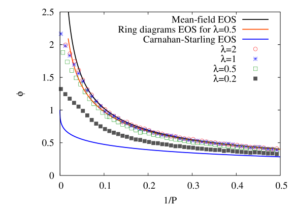
Figure 6: The equation of state of the model for different values of the shift range $\displaystyle\lambda$. Solid lines are the analytical equation of state for the mean-field case (for which it is exact), and for the monodisperse $\displaystyle 3d$ hard-sphere system (the Carnahan-Starling approximation). Points are simulation results. The equation of state sticks to the mean-field value for shifts larger than $\displaystyle\lambda=1$, except at high pressures where a glass transition prevents equilibration.

The monodisperse hard-sphere system without disorder undergoes a first order transition towards a crystal, as does the system with small values of $\displaystyle\lambda$. We have checked that nothing occurs in the equation of state for systems with shifts as small as $\displaystyle\lambda=0.15$. For smaller shifts, a weak first order transition is visible, which increases when we decrease $\displaystyle\lambda$.

IV.3 Pair correlation function

We compare the pair correlation function obtained by MC simulations with analytical results of section II. In Fig. 7 we show that for $\displaystyle g_{S}(\mathbf{x}-\mathbf{y})$ (Eq. (23)), the analytical form derived for large shifts is verified.

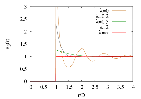
Figure 7: Pair correlation function $\displaystyle g_{S}(\mathbf{x}-\mathbf{y})$ (Eq. (23)) of a system of $\displaystyle N=864$ particles with several values of $\displaystyle\lambda$.

For finite $\displaystyle\lambda$, the usual structure of the $\displaystyle 3d$ hard-sphere model appears gradually as we reduce $\displaystyle\lambda$.

V Dynamic glass transition

In this section, we show that in $\displaystyle d=3$, we observe numerically the presence of a dynamic glass transition at finite pressure, and we study some dynamical properties close to the transition. A numerical simulation cannot exclude that the transition pressure scales with the system size (for example as $\displaystyle P_{c}\sim\ln N$), but we have given arguments in the previous sections that favor the finite-$\displaystyle P_{c}$ scenario. Note that, on the contrary, we expect that the Kauzmann pressure $\displaystyle P_{K}$ might well scale as $\displaystyle\log N$, but we shall not try to prove this in this paper.

Our model allows to study various interesting aspects of the dynamic glass transition. First, we can follow the qualitative evolution of the glass transition from mean-field to finite-dimensions. In particular we ask if we can find in the mean-field limit generic features of the mode-coupling theory, and try to see where these features break down as we move away from mean-field. Secondly, as we can generate equilibrium mean-field configurations at pressures larger than the dynamic glass transition, we can numerically access any desired property in the region between dynamic and equilibrium transitions $\displaystyle P_{c}<P<P_{K}$ (but only at infinite $\displaystyle\lambda$).

V.1 Dynamic glass transition

As is well known, mean field approximations give a dynamic transition (e.g. the mode-coupling transition) which is in fact avoided, thanks to activated processes. Here the situation is conceptually more clear: for $\displaystyle\lambda=\infty$ we expect activated processes to be absent, and for finite $\displaystyle\lambda$ we expect them to destroy any pure dynamic transition. For sufficiently large $\displaystyle\lambda$, one may expect that the trace of the dynamic transition is quite clear. The (avoided) dynamic transition pressure will still have a dependence on the range, since even the non-activated dynamics depends on the $\displaystyle\lambda$.

To specify this glass transition we look at three standard quantities: relaxation time, diffusion coefficient and dynamic susceptibility $\displaystyle\chi_{4}(t)$. First we look at the relaxation time of the system obtained from a two-time correlation function:

$$C(q,t)=\frac{1}{3N}\sum_{i=1}^{N}\sum_{\alpha=1}^{d}\cos\left(q(\mathbf{x}_{i}^{\alpha}(0)-\mathbf{x}_{i}^{\alpha}(t))\right)$$ (74)

The curves shown is this article were obtained with $\displaystyle q=\pi$. The relaxation time is defined by the time rescaling that gives the best time-pressure superposition in the $\displaystyle\alpha$ regime as shown in Fig. 8.

Figure 8: Left Two-time correlation Eq. (74) for the mean-field model for densities between $\displaystyle\phi=0.531$ and $\displaystyle\phi=1.7478$. There is a plateau appearing upon compression, and the time needed to escape this plateau increases strongly with pressure, signaling the existence of a dynamic glass transition. Right: Same data rescaled by the relaxation time $\displaystyle\tau_{\alpha}$. For high densities, time-density superposition holds.

The relaxation time shows a super-Arrhenius dependence with pressure (Fig. 9), and seems to diverge for a finite pressure (or density) value, which is characteristic of a fragile glass former. This is independent of the range of the disorder. Varying $\displaystyle\lambda$ from $\displaystyle\infty$ to $\displaystyle 0.2$ increases the glass transition pressure $\displaystyle P_{d}$ by at most 50%, while the transition density $\displaystyle\phi_{d}$ drops by almost a factor 2. This is to be related to the large shift in the equation of state as we go from a mean-field to a $\displaystyle 3d$ system, as shown in the previous section .

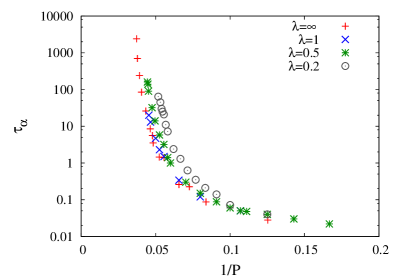
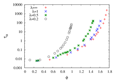
Figure 9: Left: Relaxation time $\displaystyle\tau_{\alpha}$ as a function of the pressure for several values of $\displaystyle\lambda$. The relaxation is clearly super-Arrhenius, and there is a divergence at a finite pressure for $\displaystyle\lambda=\infty$. For finite $\displaystyle\lambda$, the (apparent) dynamic transition pressure (the analogue of the Mode-coupling transition) slowly decreases when $\displaystyle\lambda$ decreases. Right: Relaxation time $\displaystyle\tau_{\alpha}$ as a function of the density. The glass transition density shows a much broader change with the range of the disorder.

The same divergence is found for the diffusion coefficient $\displaystyle D$. In Fig. 10, we plot the relation between $\displaystyle D$ and $\displaystyle\tau_{\alpha}$, showing a weak violation of the Stokes-Einstein relation, which is commonly observed for supercooled liquids. Note that this curve shows no dependence on $\displaystyle\lambda$, and extrapolates smoothly to the mean-field limit, which is quite remarkable, as the violation of Stokes-Einstein relation is often explained by the existence of dynamic heterogeneities, which depend on $\displaystyle\lambda$.

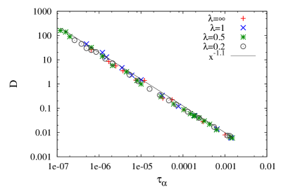
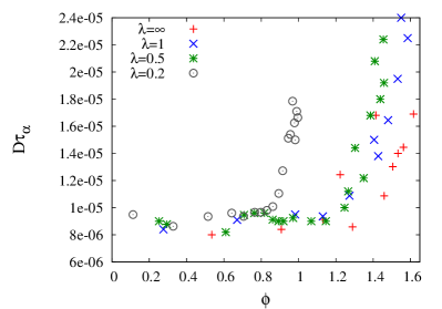
Figure 10: Left Diffusion coefficient as a function of the relaxation time for several values of $\displaystyle\lambda$. The diffusion coefficient indicates a glass transition at the same density than the relaxation time. Right Evolution of the product $\displaystyle D\tau_{\alpha}$ with density. The Stokes-Einstein relation predicts a constant $\displaystyle D\tau_{\alpha}$.

A natural quantity to study in a fragile glass former is the $\displaystyle\chi_{4}(t)$ susceptibility, a measure of dynamic heterogeneities. It is defined as the variance of the correlation $\displaystyle C$:

$$\chi_{4}(t)=N(<C(q,t)^{2}>-<C(q,t)>^{2})$$ (75)

For fragile glass former, this quantity exhibits a peak on a time scale $\displaystyle\sim\tau_{\alpha}$ with a height that sharply increases when approaching the glass transition from the liquid (low pressure) side. For pressures above the dynamic glass transition (if there is one), we expect $\displaystyle\chi_{4}(t)$ to saturate to a plateau for a time $\displaystyle\sim\tau_{\beta}$, the characteristic time of the $\displaystyle\beta$-relaxation, with a height that increases closer to the dynamic transition. When $\displaystyle\lambda$ is finite, we cannot reach the glass region, as it is impossible to equilibrate a system with an infinite relaxation time $\displaystyle\tau_{\alpha}$. However, when $\displaystyle\lambda\to\infty$, we can use the ’planted-configuration’ ensemble mentioned above to generate an equilibrium configuration even at a pressure larger than the dynamic glass transition pressure.

A typical result in the mean-field limit of our model for $\displaystyle\chi_{4}(t)$ is shown in Fig. 11. The two expected behaviors – growth from above and from below – are observed, indicating that we crossed a dynamic glass transition. The location of this qualitative change coincides with the point where the relaxation time seems to diverge, and also to the analytic estimate of the transition pressure we give below.

The dependence of $\displaystyle\chi_{4}(t)$ on $\displaystyle\lambda$ (at a given relaxation time) again shows little difference between the $\displaystyle\lambda=1$ and the mean-field cases (see Fig. 11). Further from mean-field, the height of $\displaystyle\chi_{4}(t)$ depends on $\displaystyle\lambda$, indicating a clear enhancement of the heterogeneities when we get close to the $\displaystyle 3d$ system. This is consistent with the idea that a long ranged disorder correlates large regions and thus inhibits heterogeneities occurring on smaller scales.

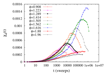
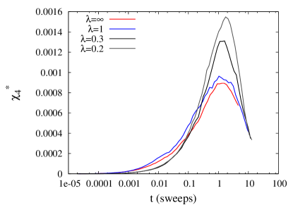
Figure 11: Left: Dynamic susceptibility $\displaystyle\chi_{4}(t)$ (75) for the mean-field model at several densities. The peak position and value grow rapidly on approaching to the glass transition. Right: $\displaystyle\chi_{4}(t)$ with different values of the range of random shifts $\displaystyle\lambda$, for equal relaxation times. Going from $\displaystyle\lambda=\infty$ to $\displaystyle\lambda=1$ does not affect the dynamic heterogeneities, while for smaller values of $\displaystyle\lambda$ (closer to finite a dimensional system), heterogeneities increase strongly.

We can infer the location of the transition by considering the divergence of the peak value $\displaystyle\chi_{4}^{*}$ of the dynamic susceptibility. This leads to the results compatible with those obtained from the relaxation time. We plotted the density dependence of the peak value $\displaystyle\chi_{4}^{*}$ in Fig. 12. Note that in the mean-field case, the divergence can be observed on both sides of the glass transition.

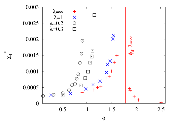
Figure 12: Peak of the dynamic susceptibility $\displaystyle\chi_{4}^{*}$ as a function of the density for several values of $\displaystyle\lambda$. This quantity shows a slight difference between $\displaystyle\lambda=1$ and the mean-field model.

It is striking that, for all these quantities, the mean-field behavior seems to be quite close to the $\displaystyle 3d$ hard-sphere model. There is no dramatic change between $\displaystyle\lambda\to\infty$ and $\displaystyle\lambda=1$. This is also probably true for other choices of the potential $\displaystyle V$, suggesting that one can create very simply a mean-field caricature of any finite-dimensional glass former by adding random shifts with a range of the order of the range of the potential.

V.2 The approach to the dynamic transition

The mode-coupling approximation predicts that the timescale $\displaystyle\tau_{\alpha}$ diverges algebraically with the distance to the glass transition density $\displaystyle\phi_{c}$ with an exponent $\displaystyle-\gamma$.

$$\tau_{\alpha}\sim\left(\frac{\phi-\phi_{c}}{\phi_{c}}\right)^{-\gamma}$$ (76)

In real life, the mode-coupling transition becomes at best a crossover, and the question is to what extent should one believe, and in what temperature-pressure range, extrapolations within mode-coupling functional forms. In our case, we also expect a divergence in the limit $\displaystyle\lambda=\infty$. What is interesting about this model, is that we may make $\displaystyle\lambda$ gradually smaller and follow the transition as it becomes a crossover, and keep track on the interpolations as they become less and less obvious, right down to the original particle model.

In order to test the behavior (76), we have to fit our simulation data with two free parameters $\displaystyle\phi_{c}$ and $\displaystyle\gamma$. In practice, this is a delicate task as one needs to have a relaxation time running over many decades to be able to chose unambiguously the couple $\displaystyle\{\phi_{c},\gamma\}$ (see for example PhysRevLett.105.199605 ). A way to help this procedure is to look at the four-point dynamic susceptibility $\displaystyle\chi_{4}(t)$. Within MCT, the maximum $\displaystyle\chi_{4}^{*}$ should diverge berthier2007spontaneous2 like $\displaystyle\chi_{4}^{*}(\phi)\sim\left(\frac{\phi-\phi_{c}}{\phi_{c}}\right)^{-1}$ . This gives us an independent measure of the $\displaystyle\gamma$ exponent, using the relation $\displaystyle\chi_{4}^{*}\sim\tau_{\alpha}^{1/\gamma}$ if there is a region where mode-coupling scaling holds. We can then look for the pair of parameters $\displaystyle\{\phi_{c},\gamma\}$ giving the best fit for both measures.

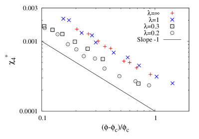
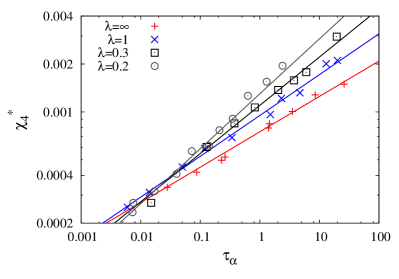
Figure 13: Left: Peak of the dynamic susceptibility $\displaystyle\chi_{4}^{*}$ as a function of the distance to the dynamic glass transition for different values of $\displaystyle\lambda$. The MCT-like scaling $\displaystyle\left(\frac{\phi-\phi_{c}}{\phi_{c}}\right)^{-1}$ is clearly visible. Right: $\displaystyle\chi_{4}^{*}$ as a function of $\displaystyle\tau_{\alpha}$ in the same regime. The power law relation obtained in MCT also seems to hold here for every values of $\displaystyle\lambda$.

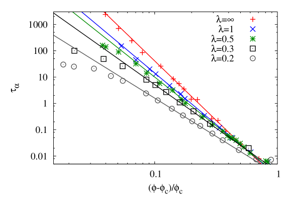
Figure 14: $\displaystyle\tau_{\alpha}$ as a function of $\displaystyle\frac{\phi-\phi_{c}}{\phi_{c}}$ for $\displaystyle\phi_{c}$ giving the broadest range of densities verifying MCT-like behaviour. The agreement is perfect for values of $\displaystyle\lambda$ down to $\displaystyle 0.5$, whereas for $\displaystyle\lambda=0.2$, the dynamic transition seems to be missed.

The results are shown in Fig 13 and Fig. 14. We get an excellent agreement with power law divergence on 6 decades of relaxation time for the mean-field model, as expected. For small values of $\displaystyle\lambda$, however, we observe a deviation to the power law scaling when we get close to the transition, presumably due to activated processes, a fact that is well attested for a $\displaystyle 3d$ binary hard sphere system PhysRevLett.102.085703 . This seems to confirm the idea that mean field theories give correct qualitative features for the relaxation time, but only over a limited range of density not too close to the glass transition. Quite interestingly, intermediate values of $\displaystyle\lambda$ show a good power-law scaling up to $\displaystyle\lambda=1$, and for $\displaystyle\lambda>1$ we were not able to observe any evidence of activation within the range of relaxation times that are reachable with our simulations.

One would like to take these simulations all the way down to $\displaystyle\lambda=0$. Unfortunately, this is not possible with a monodisperse system, but one can use a bidisperse system and follow the same steps. This is what is done in Fig. 15. Here we see that the effect is more clear: in term of relaxation time, the algebraic divergence is followed on two decades when $\displaystyle\lambda=0$, but extends to more than three decades when $\displaystyle\lambda=1$.

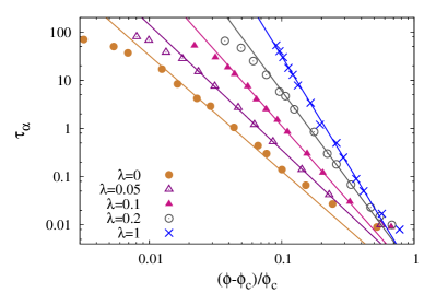
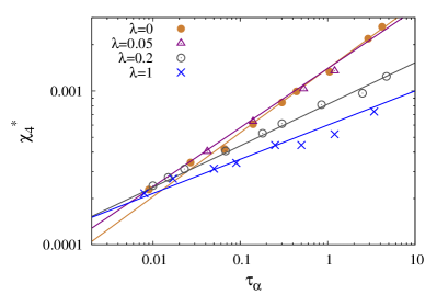
Figure 15: Left: $\displaystyle\tau_{\alpha}$ as a function of $\displaystyle\frac{\phi-\phi_{c}}{\phi_{c}}$ for $\displaystyle\phi_{c}$ giving the broadest range of densities verifying MCT-like behaviour. The agreement is perfect for values of $\displaystyle\lambda$ down to $\displaystyle 0.5$, whereas for $\displaystyle\lambda=0.2$, the dynamic transition seems to be missed.

In figure 16 we show the behavior of the extrapolated dynamical transition density and the $\displaystyle\gamma$ exponent as a function of $\displaystyle\lambda$. We observe that as $\displaystyle\lambda$ is lowered, these values continuously approach the known values for $\displaystyle 3d$ systems, both in the monodiperse van1994glass and in the bidisperse case PhysRevLett.102.085703 .

Figure 16: The values of the parameters of the MCT-like divergence, for different values of $\displaystyle\lambda$, in the monodisperse (left) and bidisperse (right) cases. These quantities show a continuous behavior from the $\displaystyle 3d,\;\lambda=0$ system to the mean field $\displaystyle\lambda=\infty$ one.

The relaxation curves for the correlations contain information beyond that of the timescale $\displaystyle\tau_{\alpha}$. The shape of the relaxation curves does depend on the range of the disorder, as is presented on Fig. 17, with the $\displaystyle\beta$-relaxation part becoming slower when $\displaystyle\lambda$ decreases, both in the case of monodisperse and of bidisperse systems. There is no visible difference between $\displaystyle\lambda=1$ and $\displaystyle\lambda=\infty$, yet another indication that for this range of disorder, the system behaves in a mean-field manner. For small $\displaystyle\lambda$, we do not observe a complete separation between $\displaystyle\alpha$ and $\displaystyle\beta$-relaxations, and the plateau is not well defined. These features however should strongly depend on the microscopic dynamics, and it is known that Monte-Carlo dynamics leads to a longer $\displaystyle\beta$-relaxation than molecular dynamics (see for example kob2002supercooled ).

Remarkably, the $\displaystyle\alpha$-relaxation shape is almost insensitive to the value of $\displaystyle\lambda$ in the monodisperse case. We can just barely notice an increase of the slope when $\displaystyle\lambda$ gets smaller, a feature that appears much more clearly in the binary mixture case, as we can access lower $\displaystyle\lambda$ values.

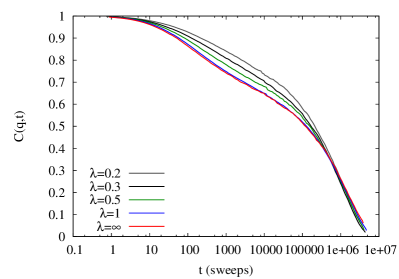
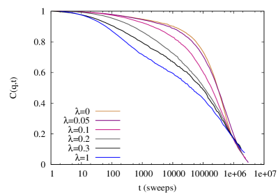
Figure 17: Relaxation curves $\displaystyle C(q,t)$ with different values of the range of random shifts $\displaystyle\lambda$, for equal relaxation times. Left: monodisperse case. The main evolution while tuning $\displaystyle\lambda$ is a lengthening the $\displaystyle\beta$-relaxation. Right: Bidisperse case. The evolution is emphasized here. The shape of the $\displaystyle\alpha$-relaxation depends varies strongly between the mean-field case and small values of $\displaystyle\lambda$.

V.3 Small or large exponent?

We wish to stress again that our goal is this work is to perform a data analysis of the same type as performed with MCT, and in particular we wanted to have an exponent $\displaystyle\gamma$ that fits the divergence of $\displaystyle\tau_{\alpha}$ on the broadest possible range and satisfies the relation between $\displaystyle\chi_{4}^{*}$ and $\displaystyle\tau_{\alpha}$. It is clear that by relaxing the constraint given by $\displaystyle\chi_{4}^{*}$ , we can fit the divergence of $\displaystyle\tau_{\alpha}$ on a broader range, and possibly on the whole available range, just by taking an exponent of the order of four, and a larger density for the divergence point (see for instance PhysRevLett.105.199605 ).

Indeed, if one looks at the relation $\displaystyle\chi_{4}^{*}$ versus $\displaystyle\tau_{\alpha}$ very close to the transition (something we have not done here but can be found in Fig. 3 of Brambilla et al. PhysRevLett.102.085703 ), one can fit the relation with a larger $\displaystyle\gamma$ on a restricted range.

Then, one can legitimately think that the exponent $\displaystyle\gamma\simeq 4.5$ we find in the mean-field limit is also the one of the $\displaystyle 3d$ hard sphere system, as long as one accepts to relax the constraint on the (mode-coupling inspired) relation of $\displaystyle\chi_{4}^{*}$ versus $\displaystyle\tau_{\alpha}$. Therefore, what our work proves is that, provided we restrict ourselves to orthodox MCT fitting, the glass transition is more and more mode-coupling-like when we approach mean-field and the part of mode-coupling divergence which is observed in finite dimension is somehow a shadow of the mean-field one. What is appealing in this point of view is that the analysis gives for the $\displaystyle 3d$ bidisperse case an exponent $\displaystyle\gamma\simeq 2.5$, which is compatible with what has already been found in experiments and simulations of comparable systems PhysRevE.58.6073 ; PhysRevLett.102.085703 ; el2009dynamic , and is reasonably close to the real MCT (not only its phenomenology) for a monodisperse system van1993glass .

V.4 Analytic estimation of the dynamic transition

One quick way to determine dynamic (mode coupling-like) transition points, is to make a static calculation of the equilibrium state, considered as an ensemble of metastable ergodic components; or, equivalently, to look for the lowest pressure at which the effective potential (free-energy at fixed distance between configurations) still has two minima.

In Appendix A we do this, leading to the determination in the figure below:

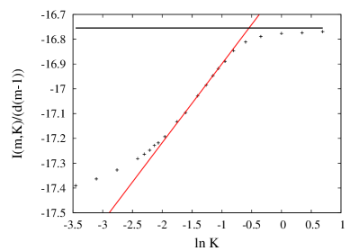
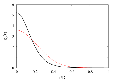
Figure 18: Left: The function defined in Eq.(95), in terms of the ”cage size” parameter $\displaystyle K$, for $\displaystyle m=0.96$. The solution for the transition pressure is obtained by searching for the point with the largest gradient, which is $\displaystyle 1/\rho_{d}$. One also obtains the estimated cage size at this point. Right: Density profiles of a single particle in its cage, defined by Eq. (77), obtained from simulations (in black), and from analytical approach with a Gaussian ansatz (in red).

The estimated transition density is $\displaystyle\phi_{d}=2^{-d}\rho_{d}=1.65$ (see left-hand side of figure 18) to be compared with the value estimated numerically $\displaystyle\phi_{d}=1.82$. Note that the analytic computation is not exact because it relies on a Gaussian approximation.

The estimated cage size is also consistent with the simulated values. In the right-hand side figure 18, we plot the quantity:

$$g_{0}(\mathbf{r})=\frac{1}{N}<\sum_{i}\delta\left[(\mathbf{x}_{i}-<\mathbf{x}_{i}>)-\mathbf{r}\right]>$$ (77)

which is as the density profile of a single particle in its cage, and is the long time limit of the so-called van Hove self-correlation function.

VI Onset Pressure

A decade ago, Sastry et al. introduced a temperature scale $\displaystyle T_{on}>T_{g}$ in supercooled liquids, the so-called onset temperature sastry1998signatures . They noticed that in a Lennard-Jones binary mixture, the energy of the inherent structures (the configurations reached after a quench at $\displaystyle T=0$) associated with equilibrium configurations at a temperature $\displaystyle T$ shows a crossover from a roughly constant value above $\displaystyle T_{on}$ to a regime where it decreases when $\displaystyle T$ decreases. They argued that this temperature is the one at which the dynamics becomes landscape-influenced, with a super-Arrhenius dependence of the relaxation time. It was a few years later argued brumer2004mean that there is a connection between $\displaystyle T_{on}$ and the computed mode-coupling density temperature $\displaystyle T_{c}$, opening the possibility that in mean-field systems $\displaystyle T_{on}$ and $\displaystyle T_{g}(=T_{c})$ might coincide. The question is legitimate, since one expects that for the spherical $\displaystyle p$-spin glass, the two temperatures do indeed coincide.

In this section, we show that this connection does not exist for our model. Because we are dealing with hard spheres, an inherent structure is the (infinite pressure) configuration reached after a rapid compression process, like the one introduced in stillinger1964systematic . In figure  19 we plot the inherent structure density reached after such a process, in terms of the initial density, for the model with $\displaystyle\lambda=\infty$ . The crossover, corresponding to the ‘onset density’ (which is the relevant quantity for hard spheres, instead of temperature, see previous section) is clearly visible. The dynamic transition in this mean-field limit ($\displaystyle d=3$) occurs at density $\displaystyle\phi_{g}=1.82$, while we find here $\displaystyle\phi_{on}\simeq 1.15$. Because $\displaystyle\phi_{g}$ is a well defined quantity here, we see beyond doubt that both densities do not coincide.

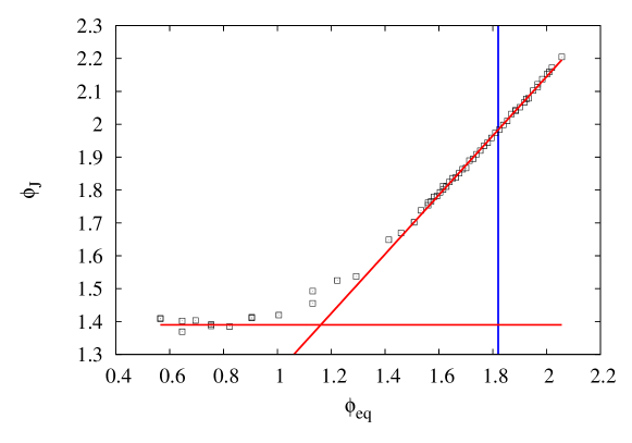
Figure 19: Inherent structure density $\displaystyle\phi_{J}$ as a function of the equilibrium liquid density $\displaystyle\phi_{eq}$. The crossover density is clearly different from the dynamic glass transition point, indicated by the vertical blue line.

As expected, the crossover density coincides with the point where the relaxation (74) starts to show a shoulder. Thus, also in the mean-field limit, $\displaystyle\phi_{on}$ marks the onset of a qualitative change in the dynamics (see Fig.8), which becomes landscape influenced.

VII Conclusions

We have introduced an approximation scheme for particle systems that is close in spirit to the Mode-Coupling approximation, but has the advantage that one may construct a continuous range of models, with at one end the original one, and at the other end one for which the approximation is exact. The approximation becomes better at higher dimensionality of space, everything else remaining equal.

As it stands, the present scheme is derived from the microscopic model. This was originally the case also with the Mode-Coupling equations, although the standard practice has become to modify freely the interactions in such a way as to obtain the observed static structure factor and transition temperature or pressure. In our case, the analogous procedure would be to substitute the true potential by one based on the pair correlation function (23)

$$V_{eff}=-T\ln[g(r)]$$ (78)

We have not tried this strategy.

In this paper we have not discussed the possible static Kauzmann transition, and we suspect that it might happen at divergent pressures, of the order of $\displaystyle\ln\lambda$, i.e. divergent in the mean-field limit.

By following the model from the original problem to its mean-field limit, we have used the present construction to give new arguments on the existence of a vestige of the genuine mean-field dynamic transition, following a mode-coupling-like behavior. We also argued conclusively that the ‘onset’ temperature (or pressure) should not be identified with the dynamic transition. More generally, one may follow this strategy to decide whether features found in true system that one ‘explains’ within random first order theory, really extrapolate to the corresponding feature in the limit in which the theory is exact.

Appendix A: An estimation of the dynamical transition pressure from replicas

Physical discussion

The dynamic glass transition is related to the existence of an exponential number of amorphous metastable states. Above a given dynamic glass transition density $\displaystyle\phi_{d}$, the liquid phase can be seen as the sum of all these states.

To derive the properties of the model at high density in order to test the above scenario, we will study the partition function of $\displaystyle m$ copies of the original system:

$$Z_{m}=\int\prod_{\alpha=1}^{m}\prod_{k}\text{d}\mathbf{x_{k}}^{\alpha}\exp\left(-\sum_{\alpha=1}^{m}\sum_{ij}V(\mathbf{x_{i}}^{\alpha}-\mathbf{x_{j}}^{\alpha}-\mathbf{A_{ij}})\right)$$ (79)

The idea is the following monasson1995structural ; mezard1996tentative ; mezard1999thermodynamics ; mezard1999first : if we force the $\displaystyle m$ copies to be close one another by adding a small coupling term between them, we can expect that if we study the system at a density higher than $\displaystyle\phi_{d}$, and switch off the coupling after taking the thermodynamic limit, the $\displaystyle m$ copies will be confined in the same metastable state.

This is done in practice by looking at the entropy of the replicated system:

$$S=\overline{\ln Z_{m}}=\lim_{n\to 0}\frac{1}{n}\left(\overline{Z_{m}^{n}}-1\right)$$ (80)

where we use the replica trick to average over disorder the logarithm of $\displaystyle Z_{m}$. Looking more closely to $\displaystyle\overline{Z_{m}^{n}}$, we see that it can be interpreted as the partition function of $\displaystyle N$ ‘molecules’ $\displaystyle\underline{\mathbf{x_{i}}}=\{\mathbf{x}_{i}^{1},...,\mathbf{x}_{i}^{nm}\}$ made of $\displaystyle nm$ spheres:

$$\begin{array}[]{rl}\overline{Z_{m}^{n}}&=\int\prod_{ij}\text{d}\mathbf{A_{ij}}P(\mathbf{A_{ij}})\int\prod_{\alpha=1}^{mn}\prod_{k}\text{d}\mathbf{x_{k}}^{\alpha}\exp\left(-\sum_{\alpha=1}^{mn}\sum_{ij}V(\mathbf{x_{i}}^{\alpha}-\mathbf{x_{j}}^{\alpha}-\mathbf{A_{ij}})\right)\\ &=\int\prod_{k}\text{d}\underline{\mathbf{x_{k}}}\prod_{ij}\int\text{d}\mathbf{A_{ij}}P(\mathbf{A_{ij}})\exp\left(-\sum_{\alpha=1}^{mn}\sum_{ij}V(\mathbf{x_{i}}^{\alpha}-\mathbf{x_{j}}^{\alpha}-\mathbf{A_{ij}})\right)\end{array}$$ (81)

Then, using standard liquid theory techniques, we are able to write the entropy Eq. (80) as a functional of the density of molecules $\displaystyle\rho(\underline{\mathbf{x}})$. The metastable states of the system are then the maxima of this entropy with respect to $\displaystyle\rho(\underline{\mathbf{x}})$ when $\displaystyle m=1$, which we expect to couple replicas.

Replicated canonical formalism

We have to study the following partition function Eq. (81). Introducing $\displaystyle\underline{\mathbf{x_{i}}}=\{\mathbf{x_{i}}^{1},...,\mathbf{x_{i}}^{nm}\}$, we can see Eq. (81) as the partition function of a $\displaystyle N$ molecules interacting via a potential $\displaystyle\tilde{V}$ such that:

$$\left[1+\overline{f}_{r}(\underline{\mathbf{x}}-\underline{\mathbf{y}})\right]=\exp\left(-\tilde{V}(\underline{\mathbf{x}}-\underline{\mathbf{y}})\right)=\int P(\mathbf{A})\text{d}\mathbf{A}\exp\left(-\sum_{\alpha=1}^{mn}\sum_{ij}V(\mathbf{x}^{\alpha}-\mathbf{y}^{\alpha}-\mathbf{A})\right)$$ (82)

Each ‘molecule’ $\displaystyle\underline{\mathbf{x_{i}}}$ is made of $\displaystyle n$ independent sets of $\displaystyle m$ coupled (in the same state) original particles. Then, Eq. (81) reads:

$$\overline{Z_{m}^{n}}=\int\prod_{i}\text{d}\underline{\mathbf{x_{i}}}\prod_{ij}\left[1+\overline{f}_{r}(\underline{\mathbf{x_{i}}}-\underline{\mathbf{x_{j}}})\right]$$ (83)

We wish to do a Mayer expansion like in the non-replicated case, but we cannot add a convenient combinatoric prefactor in (83), as we do not know what it should be a priori. However the specific properties of the random-shift model allows us to do a canonical treatment of the partition function as we show in the following. Introducing the density of molecules $\displaystyle\rho(\underline{\mathbf{x}})$ by:

$$\rho(\underline{\mathbf{x}})=\sum_{i}\delta(\underline{\mathbf{x}}-\underline{\mathbf{x_{i}}})$$ (84)

we can rewrite $\displaystyle\overline{Z_{m}^{n}}$ as:

$$\overline{Z_{m}^{n}}=\int\text{d}\underline{\mathbf{x_{i}}}\int\text{D}[\rho(\mathbf{x})]\delta\left(\rho(\mathbf{\underline{x}})-\sum_{i}\delta(\mathbf{\underline{x}}-\mathbf{\underline{x}}_{i})\right)\exp\left[\frac{1}{2}\int\text{d}\mathbf{\underline{x}}\text{d}\mathbf{\underline{y}}\rho(\mathbf{\underline{x}})\rho(\mathbf{\underline{y}})\ln\left[1+\overline{f}_{r}(\underline{\mathbf{x}}-\underline{\mathbf{y}})\right]\right]$$ (85)

We may now exponentiate the $\displaystyle\delta$ constraint at the cost of adding a second field $\displaystyle\hat{\rho}$, and integrating over the $\displaystyle\underline{\mathbf{x_{i}}}$’s:

$$\begin{array}[]{rl}\overline{Z_{m}^{n}}=\int&\text{D}[\rho(\underline{\mathbf{x}})]\text{D}[\hat{\rho}(\underline{\mathbf{x}})]\\ &\exp\left\{i\int\text{d}\underline{\mathbf{x}}\hat{\rho}(\underline{\mathbf{x}})\rho(\underline{\mathbf{x}})+N\ln\int\text{d}\underline{\mathbf{x}}e^{-i\hat{\rho}(\underline{\mathbf{x}})}+\frac{1}{2}\int\text{d}\underline{\mathbf{x}}\text{d}\underline{\mathbf{y}}\rho(\underline{\mathbf{x}})\rho(\underline{\mathbf{y}})\ln\left[1+\overline{f}_{r}(\underline{\mathbf{x}}-\underline{\mathbf{y}})\right]\right\}\end{array}$$ (86)

The next important step is to look more closely at the function $\displaystyle\overline{f}_{r}(\mathbf{\underline{x}}-\mathbf{\underline{y}})$, as we did in the non-replicated case. In the integral of Eq. (82), the exponential of the potential $\displaystyle V$ vanishes $\displaystyle 1$ whenever the two molecules in $\displaystyle\mathbf{\underline{x}}$ and $\displaystyle\mathbf{\underline{y}}+\mathbf{A}$ overlap, and gives $\displaystyle 1$ otherwise. Then we have:

$$-nm\frac{v_{d}}{V}\leq\overline{f}_{r}(\underline{\mathbf{x}}-\underline{\mathbf{y}})\leq-\frac{v_{d}}{V}$$ (87)

Thus, by expanding the logarithm, we get:

$$\begin{array}[]{rl}\overline{Z_{m}^{n}}=\int&\text{D}[\rho(\underline{\mathbf{x}})]\text{D}[\hat{\rho}(\underline{\mathbf{x}})]\\ &\exp\left\{i\int\text{d}\underline{\mathbf{x}}\hat{\rho}(\underline{\mathbf{x}})\rho(\underline{\mathbf{x}})+N\ln\int\text{d}\underline{\mathbf{x}}e^{-i\hat{\rho}(\underline{\mathbf{x}})}+\frac{1}{2}\int\text{d}\underline{\mathbf{x}}\text{d}\underline{\mathbf{y}}\rho(\underline{\mathbf{x}})\rho(\underline{\mathbf{y}})\overline{f}_{r}(\underline{\mathbf{x}}-\underline{\mathbf{y}})\right\}\end{array}$$ (88)

We wish then to evaluate this integral by saddle point with respect to the fields $\displaystyle\rho$ and $\displaystyle\hat{\rho}$ (because each term in the exponential is of order $\displaystyle N$, including the last one, due to the value of $\displaystyle f$). This gives:

$$\begin{array}[]{rl}\rho(\mathbf{\underline{x}})&=N\frac{e^{-i\hat{\rho}(\mathbf{\underline{x}})}}{\int\text{d}\mathbf{\underline{x}}e^{-i\hat{\rho}(\mathbf{\underline{x}})}}\\ \hat{\rho}(\mathbf{\underline{x}})&=i\int\text{d}\mathbf{\underline{y}}\rho(\mathbf{\underline{y}})\overline{f}_{r}(\mathbf{\underline{x}}-\mathbf{\underline{y}})\end{array}$$ (89)

Thus, the logarithm of the partition function is:

$$\ln\overline{Z_{m}^{n}}=-\int\text{d}\mathbf{\underline{x}}\rho(\mathbf{\underline{x}})\ln\rho(\mathbf{\underline{x}})+\frac{1}{2}\int\text{d}\mathbf{\underline{x}}\text{d}\mathbf{\underline{y}}\rho(\mathbf{\underline{x}})\rho(\mathbf{\underline{y}})f(\mathbf{\underline{x}}-\mathbf{\underline{y}})+N\ln N$$ (90)

We wish to stress the similarity of Eq. (90) with Eq. (14). In fact the average over disorder does exactly the same job for the replicated liquid than for the bare non-replicated liquid: it disallows ‘three-molecule effective interactions’, just like in a high-dimensional system.

Location of the dynamic transition, within the Gaussian ansatz

We may obtain an approximation for $\displaystyle\rho$ by assuming it has a Gaussian form. Of course, this ansatz will not be a solution of the full saddle point equation Eq. (89), but we can still extremize the entropy Eq. (90) within this ansatz. A natural choice is the ansatzparisi2010mean :

$$\rho(\mathbf{\underline{x}})=\frac{N}{V^{n}}\prod_{\gamma=1}^{n}\int\text{d}\mathbf{X_{\gamma}}\frac{1}{(2\pi K)^{md/2}}\exp\left[\sum_{\alpha=\gamma(m-1)+1}^{\gamma m}\frac{\left(\mathbf{x^{\alpha}}-\mathbf{X_{\gamma}}\right)^{2}}{2K}\right]$$ (91)

Note the similarity with the dynamic ansatz.

This is a 1-step replica symmetry breaking (1-RSB) ansatz. Injecting Eq. (91) in the partition function Eq. (90) leads to integrals exactly similar to the ones one has compute in the hard sphere system (without random shifts). This has been done in parisi2010mean . Following the computations along the lines of parisi2010mean , one finds:

$$\begin{array}[]{rl}\frac{S[\rho(\mathbf{\underline{x}})]}{N}=\ln N+1-\ln\rho-\frac{d}{2}(1-m)\ln(2\pi K)+\frac{d}{2}\ln m-\frac{d}{2}(1-m)-\frac{\rho}{2}I(m,K)\end{array}$$ (92)

where $\displaystyle I(m,K)$ is the integral:

$$I(m,K)=\int\text{d}\mathbf{X}\left[\int\text{d}\mathbf{x}\text{d}\mathbf{y}\frac{1}{(2\pi K)^{d}}\exp\left(\frac{\left(\mathbf{x}-\mathbf{X}\right)^{2}}{2K}\right)\exp\left(\frac{\mathbf{y}^{2}}{2K}\right)\chi(\mathbf{x}-\mathbf{y})\right]^{m}$$ (93)

Then, the saddle point equation on $\displaystyle K$ reads:

$$\frac{d(m-1)}{\rho}=\frac{\partial I(m,K)}{\partial\ln K}$$ (94)

Thus, there exist metastable states in the liquid phase (which is recovered in the limit $\displaystyle m\to 1$) if there is a cage size $\displaystyle K$ which verifies:

$$\frac{1}{\rho}=\lim_{m\to 1}\frac{1}{d(m-1)}\frac{\partial I(m,K)}{\partial\ln K}$$ (95)

The dynamic glass transition density is $\displaystyle\rho_{d}$, beynd which no solution to this equation can be found. It is possible to compute $\displaystyle I(m,K)$ numerically, and we find $\displaystyle\phi_{d}=2^{-d}\rho_{d}\simeq 1.65$ for $\displaystyle d=3$ (see Fig. 18), not far from the value ($\displaystyle 1.82$) found in numerical simulations. The value of $\displaystyle K$ at the transition is also comparable with what is found in the simulations (see Fig. 18).

Appendix B : Gaussian ansatz for the mean-field dynamics

VII.1 Notation

The calculation we are going to follow is quite heavy. It may be made somewhat more compact, and one may follow the analogy with the static treatment better, by using the supersymmetric notation zinn2002quantum (see kurchan1992supersymmetry ; semerjian2004stochastic ). One introduces two extra Grassmann variables $\displaystyle\theta$ et $\displaystyle\overline{\theta}$. Denoting $\displaystyle a=(t,\theta,\overline{\theta})$, the trajectories $\displaystyle\mathbf{x}(t)$ and $\displaystyle\hat{\mathbf{x}}(t)$ may be encoded in a superfield $\displaystyle\psi(a)$:

$$\psi(a)=\mathbf{x}(t)+\theta\overline{\theta}\hat{\mathbf{x}}(t)$$ (96)

Defining the operator $\displaystyle D_{a}$ as

$$D_{a}=T\frac{\partial^{2}}{\partial\theta\partial\overline{\theta}}+\theta\frac{\partial^{2}}{\partial\theta\partial t}-\frac{\partial}{\partial t}$$ (97)

we have:

$$\Phi[\mathbf{x},\hat{\mathbf{x}}]=\int\text{d}a\text{d}b\;\delta(b-a)D_{a}\left(\psi(a)-\psi(b)\right)^{2}$$ (98)

Similarly:

$$\begin{array}[]{rl}1+\overline{f}_{d}[\mathbf{x},\hat{\mathbf{x}},\mathbf{x}^{\prime},\hat{\mathbf{x}}^{\prime}]&=\int\text{d}\mathbf{A}P(\mathbf{A})\exp\left\{-\frac{1}{2}\int_{0}^{\tau}\text{d}t\;\hat{\mathbf{x}}(t)\nabla_{\mathbf{x}}V(\mathbf{x}-\mathbf{y}-\mathbf{A}))+\hat{\mathbf{y}}(t)\nabla_{\mathbf{y}}V(\mathbf{y}-\mathbf{x}-\mathbf{A})\right\}\\ &=\int\text{d}\mathbf{A}P(\mathbf{A})\exp\left\{-\frac{1}{2}\int\text{d}a\;V\left(\psi(a)-\psi^{\prime}(a)-\mathbf{A}\right)\right\}\\ &=1+\overline{f}_{d}[\psi,\psi^{\prime}]\end{array}$$ (99)

The action can be written in the following compact way:

$$\begin{array}[]{rl}\mathcal{S}\left[\rho[\psi]\right]=&\int\text{D}\psi\rho[\psi]\ln\left[\rho[\psi]\right]+\int\text{D}\psi\rho[\psi]\int\text{d}a\;\psi(a)D_{a}\psi(a)\\ &\qquad-\frac{1}{2}\int\text{D}[\psi,\psi^{\prime}]\rho[\psi]\rho[\psi^{\prime}]\overline{f}_{d}[\psi-\psi^{\prime}]-N\ln N\end{array}$$ (100)

By analogy with the statics, one may make a ‘Gaussian’ ansatz $\displaystyle\rho$ semerjian2004stochastic :

$$\rho[\psi]=\frac{\sqrt{2}}{V\;\det^{\frac{1}{2}}(\mathcal{B})}\int d{\bf{\bar{x}}}\;\exp\left[-\int dadb\;{\mathcal{B}}^{-1}(a,b)\;(\psi(a)-\mathbf{\bar{x}})(\psi(b)-\mathbf{\bar{x}})\right]$$ (101)

with

$$\mathcal{B}(a,a)=0\;\;\;\forall\;\;\;a$$ (102)

In components, the super-correlators read:

$$\displaystyle\mathcal{B}(a,b) \displaystyle= \displaystyle{B}(t_{a},t_{b})-\overline{\theta}_{a}\theta_{a}{R}(t_{b},t_{a})-{\bar{\theta}}_{b}\theta_{b}{R}(t_{a},t_{b})+{D}(t_{a},t_{b}){\bar{\theta}}_{a}\theta_{a}{\bar{\theta}}_{b}\theta_{b}$$

$$\displaystyle\mathcal{B}^{-1}(a,b) \displaystyle= \displaystyle{\tilde{B}}(t_{a},t_{b})-\overline{\theta}_{a}\theta{\tilde{R}}(t_{b},t_{a})-{\bar{\theta}}_{b}\theta_{b}{\tilde{R}}(t_{a},t_{b})+{\tilde{D}}(t_{a},t_{b}){\bar{\theta}}_{a}\theta_{a}{\bar{\theta}}_{b}\theta_{b}$$ (103)

and they are related through:

$$\int\text{d}{\bar{\theta}}_{b}\text{d}\theta_{b}\text{d}t_{b}\;\mathcal{B}(a,b)\mathcal{B}^{-1}(b,c)=\delta({\bar{\theta}_{a}}-{\bar{\theta}_{c}})\delta(\theta_{a}-{\theta_{c}})\delta(t_{a}-t_{c})$$ (104)

This inversion formula may be developed, to obtain the ”tilde” variables in terms of the ones without tilde.

In equilibrium, the fluctuation-dissipation theorem implies that $\displaystyle{\cal B}$ and $\displaystyle{\cal B}^{-1}$ take the form:

$$\displaystyle\mathcal{B}(a,b) \displaystyle= \displaystyle{B}(t_{a}-t_{b})-\overline{\theta}_{a}\theta_{a}{R}(t_{b}-t_{a})-{\bar{\theta}}_{b}\theta_{b}{R}(t_{a}-t_{b})$$

$$\displaystyle\mathcal{B}^{-1}(a,b) \displaystyle= \displaystyle{\tilde{B}}(t_{a}-t_{b})-\overline{\theta}_{a}\theta_{a}{\tilde{R}}(t_{b}-t_{a})-{\bar{\theta}}_{b}\theta_{b}{\tilde{R}}(t_{a}-t_{b})$$ (105)

where

$$R(t)=-\frac{1}{T}\frac{\partial B}{\partial t}\;\;\;;\;\;\;{\tilde{R}}(t)=-\frac{1}{T}\frac{\partial{\tilde{B}}}{\partial t}$$ (106)

where $\displaystyle R$ and $\displaystyle{\tilde{R}}$ are zero for negative time-differences, due to causality.

It is easy to show that:

$$\Phi[\mathbf{x},\hat{\mathbf{x}}]=\frac{1}{V}\int\text{d}{\bf{\bar{x}}}\;\int\text{d}a\text{d}b\;\delta(b-a)D_{a}(\psi(a)-\mathbf{\bar{x}})(\psi(b)-\mathbf{\bar{x}})$$ (107)

The super-correlator $\displaystyle\mathcal{B}$ is given by:

$$\mathcal{B}(a,b)=\int\text{D}\psi\left(\psi(a)-\psi(b)\right)^{2}\rho[\psi]$$ (108)

Inserting this ansatz in Eq. (100), we get:

$$\mathcal{S}\left(\mathcal{B}\right)=-\frac{1}{2}\text{Tr}\ln\mathcal{B}+\int\text{d}a\text{d}b\;\delta(a-b)D_{a}\mathcal{B}(a,b)-\mathcal{S}_{int}(\mathcal{B})$$ (109)

with

$$\begin{array}[]{rl}\mathcal{S}_{int}(\mathcal{B})&=\frac{1}{V^{2}\det\mathcal{B}}\int\text{D}[\psi,\psi^{\prime}]\int\text{d}\bar{\mathbf{x}}\text{d}\bar{\mathbf{y}}\\ &\quad\exp\left[-\int\text{d}a\text{d}b\;\mathcal{B}^{-1}(a,b)\left[(\psi(a)-\bar{\mathbf{x}})(\psi(b)-\bar{\mathbf{x}})+(\psi^{\prime}(a)-\bar{\mathbf{y}})(\psi^{\prime}(b)-\bar{\mathbf{y}})\right]\right]\;\overline{f}_{d}[\psi,\psi^{\prime}]\end{array}$$ (110)

The integrand is invariant with respect to independent translations of $\displaystyle{\bf x}$ and $\displaystyle{\bf y}$, because they may be absorbed into the shift $\displaystyle\mathbf{A}$, so we may write:

$$\mathcal{S}_{int}(\mathcal{B})=\frac{1}{\det\mathcal{B}}\int\text{D}[\psi,\psi^{\prime}]\;\exp\left[-\int\text{d}a\text{d}b\;\mathcal{B}^{-1}(a,b)\left[\psi(a)\psi(b)+\psi^{\prime}(a)\psi^{\prime}(b)\right]\right]\;\overline{f}_{d}[\psi,\psi^{\prime}]$$ (111)

The saddle point equation gives:

$$0=\frac{\delta\mathcal{S}}{\delta\mathcal{B}(a,b)}=-\frac{1}{2}\mathcal{B}^{-1}(a,b)+\delta(a-b)D_{a}-\frac{\delta\mathcal{S}_{int}}{\delta\mathcal{B}(a,b)}$$ (112)

with:

$$\frac{\delta\mathcal{S}_{int}}{\delta\mathcal{B}(a,b)}=\frac{1}{2}\mathcal{B}^{-1}(a,b)-\left[\mathcal{B}^{-1}\otimes\langle\psi(a^{\prime})\psi(b^{\prime})\rangle_{int}\otimes\mathcal{B}^{-1}\right](a,b)$$ (113)

and:

$$\langle\bullet\rangle_{int}=\int\text{D}\psi\int\text{D}\psi^{\prime}\bullet\rho[\psi]\rho[\psi^{\prime}]\;\overline{f}_{d}[\psi,\psi^{\prime}]$$ (114)

Making the convolution product with $\displaystyle\mathcal{B}(b,c)$, we obtain:

$$0=D_{a}\mathcal{B}(a,b)+\int\text{d}c\;\Sigma(a,c)\mathcal{B}(c,b),$$ (115)

where $\displaystyle\Sigma$ is given by

$$\Sigma(a,b)=-2\left[\mathcal{B}^{-1}\otimes\langle\psi(a^{\prime})\psi(b^{\prime})\rangle_{int}\otimes\mathcal{B}^{-1}\right](a,b),$$ (116)

also of the form (103):

$${\Sigma}(a,b)={\Sigma_{B}}(t_{a}-t_{b})-\overline{\theta}_{a}\theta_{a}{\Sigma_{R}}(t_{b}-t_{a})-{\bar{\theta}}_{b}\theta_{b}{\Sigma_{R}}(t_{a}-t_{b})$$ (117)

$\displaystyle\Sigma_{B}$ and $\displaystyle\Sigma_{R}$ satisfy also a fluctuation-dissipation relation:

$$\Sigma_{R}(t)=-\frac{1}{T}\frac{\partial\Sigma_{B}}{\partial t}$$ (118)

Because correlation and response satisfy a fluctuation-dissipation relation, we may write everything exclusively in terms of correlations:

$$\frac{\partial B(t_{a}-t_{b})}{\partial t_{a}}=-TR(t_{b}-t_{a})+\int\text{d}t_{c}\;\Sigma_{R}(t_{a}-t_{c})B(t_{c}-t_{b})-\left.\Sigma_{C}(t_{b}-t_{c})B(t_{b}-t_{c})\right|_{-\infty}^{t_{b}},$$ (119)

with:

$$\Sigma_{R}(t_{a}-t_{b})=\frac{2}{T}\int\text{d}t_{a^{\prime}}\text{d}t_{b^{\prime}}\;{R}^{-1}(t_{a}-t_{a^{\prime}})\;\frac{\partial}{\partial t_{a^{\prime}}}\langle\mathbf{x}(t_{a^{\prime}})\mathbf{x}(t_{b^{\prime}})\rangle_{int}\;{R}^{-1}(t_{b^{\prime}}-t_{b})$$ (120)

Given that, as $\displaystyle t_{a}\rightarrow t_{b}$, $\displaystyle B(t_{a}-t_{b})\sim 2T|t_{a}-t_{b}|$, we have that:

$$\begin{array}[]{rl}\frac{\partial B(t_{a},t_{b})}{\partial t_{a}}&=-TR(t_{b},t_{a})+\int\text{d}t_{c}\;\Sigma_{R}(t_{a}-t_{c})B(t_{c}-t_{b})+2T\\ 2T&=-\left.\Sigma_{B}(t_{b}-t_{c})B(t_{b}-t_{c})\right|_{-\infty}^{t_{b}},\end{array}$$ (121)

which is the result (69).