Two dimensional representation of the Dirac equation in Non associative algebra

In this note a simple extension of the complex algebra to higher dimension is proposed. Using the proposed algebra a two dimensional Dirac equation is formulated and its solution is calculated. It is found that there is a sub-algebra where the associative nature can be recovered.

Keywords: Dirac equation, non associative algebra.

1 Introduction

The physical motivation of a generalized quantum mechanics is that, although the low-energy effective theories governing the strong, electroweak, and gravitational interactions of elementary particles are believed to be described by local complex quantum field theories, attempts to construct an underlying unifying theory within the same framework have run into difficulties. Perhaps a successful unification of the fundamental forces will require one or more new ingredients at the conceptual level. One possibility, is to sacrifice the assumption of locality or of ”point” particles, as is done in string theories. A second possibility, which motivates the present work, is that a successful unification of the fundamental forces will require a generalization beyond complex quantum mechanics[1, 2, 3, 4, 5, 6, 7, 8, 9, 10, 11, 12].

In the present work, our aim, is to give a description of an algebra which can be used in a possible extension of the local complex quantum field theories. Also, a considerable emphasis is placed on the development of two dimensional Dirac equation. A number of interesting and characteristic features of the non associative algebra will be seen to emerge.

This paper is organized as follow: in the next section the description of the algebra is given. Section 3 is devoted to the study of two dimensional Dirac equation. Our conclusion will be given in section 4.

2 Number systems used in Quantum mechanics and the Generalized-$\mathbb{C}$

To determine the allowed structure of the algebra that can be used for a generalized quantum mechanics, Adler [1] introduced a number of assumptions concerning the properties of the modulus function $N$ of the number $\phi$ elements of the algebra:

$$N(0)=0$$ (1)

$$N(\phi)>0\quad\rm if\,\phi\neq 0$$ (2)

$$N(r\phi)=|r|N(\phi)\quad r\,\rm real$$ (3)

$$N(\phi_{1}+\phi_{2})\leq N(\phi_{1})+N(\phi_{2})$$ (4)

$$N(\phi_{1}\phi_{2})=N(\phi_{1})N(\phi_{2})$$ (5)

The $\phi$’s are elements of a general finite dimensional algebra over the real numbers with unit element, of the form

$$\phi=\sum_{A}r_{A}e_{A}$$

where $r_{A}$ are real numbers and the $e_{A}$ are basis elements of the algebra, obeying the multiplication law

$$e_{A}e_{B}=\sum_{C}f_{ABC}e_{C}$$

with real-number structure constants $f_{ABC}$.

With the help of Albert theorem [13], it is found that the only algebras over the reals, admitting a modulus function with Adler properties, are the reals $\mathbb{R}$, the complex numbers $\mathbb{C}$, the quaternions or Hamilton numbers $\mathbb{H}$ and the octonions or Cayley numbers $\mathbb{O}$.

However, from experimental point of view, there is no guarantee that the Adler postulate about the modulus function $N$ will be satisfied in the new energies domains. Perhaps, new physics can emerge [14]. Thus, there should be no restriction about the algebra that can be used for a possible extension of the complex algebra. The only requirement is that the expected extension should verify Adler postulate in its sub-algebra. Moreover, it is more natural, to assume a simple extension, rather than making extension to 4 dimensional or even higher. This idea will be used in our approach. In fact, we propose to use a three dimensional algebra. Our intuitive assumption is based on a geometrical approach as proposed by Descartes in describing the complex number.

Our Approach: The proposed generalization of the $\mathbb{C}$ algebra, the Generalized-$\mathbb{C}$ (G$\mathbb{C}$), is finite-dimensional non division algebra containing the real numbers $\mathbb{R}$ as a sub-algebra and has the following properties:

• A general G$\mathbb{C}$ number, q, can be written as

  $$q=a+bi+cj$$

  where

  $$\emph{a,b,c,}\in\mathbb{R}\,\rm or\,\mathbb{C}\,,$$

  and the imaginary G$\mathbb{C}$ units, $i,j$ are defined by

  $$ii=jj=-1$$

  $$ij=ji=0$$

• The addition defined as

  $$q_{1}+q_{2}=a_{1}+a_{2}+(b_{1}+b_{2})i+(c_{1}+c_{2})j\,,$$

  is associative

  $$q_{1}+(q_{2}+q_{3})=(q_{1}+q_{2})+q_{3}\,.$$

• The multiplication defined as

  $$q_{1}q_{2}=(a_{1}a_{2}-b_{1}b_{2}-c_{1}c_{2})$$

  $$+(a_{1}b_{2}+b_{1}a_{2})i$$

  $$+(a_{1}c_{2}+c_{1}a_{2})j\,,$$

  is non-associative under multiplication that is $(q_{1}q_{2})q_{3}\neq q_{1}(q_{2}q_{3})$.

• The norm of an element $q$ of G$\mathbb{C}$ is defined by

  $$N(q)=(\bar{q}q)^{1/2}=(a^{2}+b^{2}+c^{2})^{1/2}$$

  with the G$\mathbb{C}$ conjugate $q$ given by

  $$\bar{q}=a-bi-cj\,.$$

Using the properties of the G$\mathbb{C}$, a generalization of the Euler formula to three dimension can be found. In fact any $q$ can be written as

$$q=a+bi+cj=Re^{\theta(\cos(\phi)i+\sin(\phi)j)}=R\sum{(\theta(\cos(\phi)i+\sin(\phi)j))^{n}\over n!}$$

where $a=R\cos(\theta),\,b=R\sin(\theta)\cos(\phi),\,c=R\sin(\theta)\sin(\phi)$ and ${R,\theta,\phi}\in\mathbb{R}$, are the distance from the origin, the polar and the azimuthal angle in the three dimensional Euler space.

Note that, $e^{\theta(\cos(\phi)i+\sin(\phi)j)}\neq e^{\theta\cos(\phi)i}e^{\theta\sin(\phi)j}$ because the multiplication law is commutative but not assciative.

It is important to note, as we mention previously, that there exist a sub-algebra of G$\mathbb{C}$ where the probability is preserved in quantum mechanics. In this sub-algebra we must assume that the azimuthal phase $\phi$ is constant. In this case G$\mathbb{C}$ will be an associative and division sub-algebra that we call special G$\mathbb{C}$ (SG$\mathbb{C}$). Thus any two numbers in this sub-algebra can be written as

$$q_{1}=a_{1}+b_{1}i+c_{1}j=R_{1}e^{\theta_{1}(\cos(\phi)i+\sin(\phi)j)}\,,\quad q_{2}=a_{2}+b_{2}i+c_{2}j=R_{2}e^{\theta_{2}(\cos(\phi)i+\sin(\phi)j)}$$

where the phase $\phi$ is a free parameter that can be determined from physical properties. Also in this sub-algebra the product of two elements have a physical meaning that is a rotation in the Euler space

$$q_{1}q_{2}=R_{1}R_{2}e^{(\theta_{1}+\theta_{2})(\cos(\phi)i+\sin(\phi)j)}\,.$$

3 Two dimensional Dirac’s Equation in the Generalized-$\mathbb{C}$

In this section an ab initio development of the Dirac formalism in two dimension using the proposed Generalized-$\mathbb{C}$ is discussed. In fact, in $\mathbb{C}$, Dirac’s equation is often given as

$$(i\gamma^{\mu}\partial_{\mu}-m)\psi=0$$

which involves $i\in\mathbb{C}$ and thus forces the first decision point in transitioning to another mathematical algebra. For clarity, to avoid the explicit use of $i$, the most general form ($c=\hbar=1$) of Dirac’s equation is

$$\mathcal{H}\psi=(C_{\mu}\partial_{\mu})\psi=(C_{x}\partial_{x}+C_{y}\partial_{y}+C_{z}\partial_{z}+C_{t}\partial_{t})\psi=m\psi.$$ (6)

To recover the Klein-Gordon equation

$$(\nabla^{2}-\partial_{t}^{2})\psi=m^{2}\psi,$$ (7)

the following conditions must hold

$$C_{x,y,z}^{2}=1;\hskip 7.22743ptC_{t}^{2}=-1;\hskip 7.22743pt\mbox{ and }\left\{C_{\mu},C_{\nu}\right\}=C_{\mu}C_{\nu}+C_{\nu}C_{\mu}=0,\mbox{ where }\mu\neq\nu.\hskip 7.22743pt\mu,\nu=x,y,z,t$$ (8)

Equation (6) can be rewritten as

$$(\gamma^{\mu}\partial_{\mu}-m)\psi=0,\hskip 21.68121pt\mu=0,1,2,3$$ (9)

by defining

$$\gamma^{\mu}=(C_{t},C_{x},C_{y},C_{z})$$

this avoids the explicit use of an imaginary scalar. Using the following Dirac matrices, that take into account  i, j  symmetry, satisfying (8)

$\gamma^{0}\equiv\gamma^{t}\equiv C_{t}=\left(\begin{array}[]{cccc}0&j\\ j&0\end{array}\right)$

$\gamma^{1}\equiv\gamma^{x}\equiv C_{x}=\left(\begin{array}[]{cccc}0&-j\\ j&0\end{array}\right)$

$\gamma^{2}\equiv\gamma^{y}\equiv C_{y}=\left(\begin{array}[]{cccc}0&-i\\ i&0\end{array}\right)$

$\gamma^{3}\equiv\gamma^{z}\equiv C_{z}=\left(\begin{array}[]{cccccccc}1&0\\ 0&-1\end{array}\right)$

in equation(9) results in:

$$(\mathcal{H}-m)\psi=\left(\begin{array}[]{cccc}-m+\partial_{z}&-j\partial_{x}-i\partial_{y}+j\partial_{t}\\ j\partial_{x}+i\partial_{y}+j\partial_{t}&-m-\partial_{z}\end{array}\right)\left(\begin{array}[]{c}\psi_{1}\\ \psi_{2}\end{array}\right)=0$$ (10)

The solution to this equation in 1+1 dimension, $x,t$, can be found

$$\psi(x,t)=N\left(\begin{array}[]{c}{E+p\over m}\\ 1\end{array}\right)e^{j(px-Et)}\quad\,$$ (11)

as usual $p$ represent the ‘momentum’ and $E=\pm\sqrt{p^{2}+m^{2}}$ is the ‘energy’ and $N$ is a normalization factor.

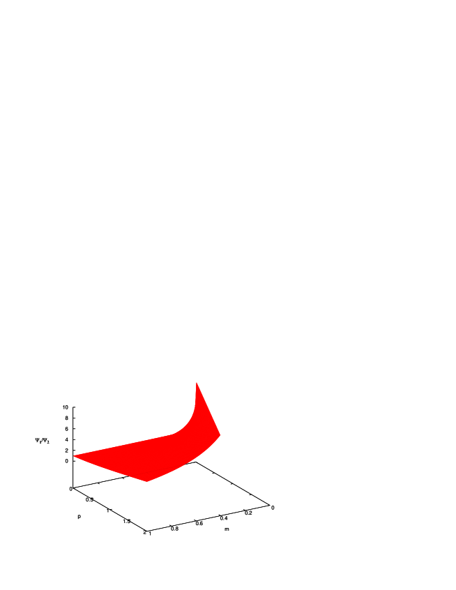
Figure 1: $\Psi_{1}/\Psi_{2}$ as function of $m$ and $p$.

The ratio $\psi_{1}/\psi_{2}$ is shown in Fig. 1. Discussion about the physical meaning of these results and application to local field theory will be left for future investigation.

4 Conclusions

We have found a two dimensional Dirac wave function in non a associative algebra. A possible criticism of the approach of this paper is that is there a physical quantities that can emerge? The intent of future articles is to contribute to the resolution of that debate. Finally we believe that such algebra merit to be explored in more physical problems.

References

- [1] see page 6 in Stephen L. Adler. Quaternion Quantum Mechanics and Quantum Fields. Oxford University Press, New York, (1995).
- [2] G. Birkhoff, J. and von Neumann, (1936). Ann. Math. 37, 823
- [3] D. Finkelstein, J. M. Jauch, S. Schiminovich, and D. Speiser. Foundations of Quaternion Quantum Mechanics. Journal of Mathematical Physics, 3(2):207–220, (1962).
- [4] Alexander Yefremov, Florentin Smarandache, and Vic Christiano. Yang-Mills Field from Quaternion Space Geometry, and its Klein-Gordon Representation. Progress in Physics, 3:42, (2007).
- [5] Igor Frenkel and Matvei Libine. Quaternion Analysis, Representation Theory and Physics. arXic, math/0711.2699v4, (2008).
- [6] O.P.S. Negi. Higher Dimensional Supersymmetry. arXic, hep-th/0608019v1, (2006).
- [7] Stefano De Leo and Pietro Rotelli. The Quaternionic Dirac Lagarangian. arXiv, hep-th/9509059v1, (1995).
- [8] Khaled Abdel-Khalek. Quaternionic Analysis. arXiv, hep-th/9607152v2, (1996).
- [9] Stephen L. Adler. Quaternionic Quantum Mechanics and Noncommutative Dynamics. arXiv, hep-th/9607008v1, (1996).
- [10] M. D. Maia. Spin and Isospin in Quaternion Quantum Mechanics. arXiv, hep-th/9904067v1, (1999).
- [11] Seema Rawat and O.P.S. Negi. Quaternion Dirac Equation and Supersymmetry. arXiv, hep-th/0701131v1, (2007).
- [12] Seema Rawat and O.P.S. Negi. Quaternionic Formulation of Supersymmetric Quantum Mechanics. arXiv, hep-th/0703161v1, (2007).
- [13] Albert A.A. (1947). Ann. Math. 35, 65
- [14] S Hamieh, J Letessier, J Rafelski, Phys.Rev.C62:064901,2000. S Hamieh, K Redlich, A Tounsi Phys.Lett.B486:61-66,2000.