Hole burning in a nanomechanical resonator coupled to a Cooper pair box

Abstract

We propose a scheme to create holes in the statistical distribution of excitations of a nanomechanical resonator. It employs a controllable coupling between this system and a Cooper pair box. The success probability and the fidelity are calculated and compared with those obtained in the atom-field system via distinct schemes. As an application we show how to use the hole-burning scheme to prepare (low excited) Fock states.

,

1 Introduction

Nanomechanical resonators (NR) have been studied in a diversity of situations, as for weak force detections [1], precision measurements [2], quantum information processing [3], etc. The demonstration of the quantum nature of mechanical and micromechanical devices is a pursued target; for example, manifestations of purely nonclassical behavior in a linear resonator should exhibit energy quantization, the appearance of Fock states, quantum limited position-momentum uncertainty, superposition and entangled states, etc. NR can now be fabricated with fundamental vibrational mode frequencies in the range MHz – GHz [4, 5, 6]. Advances in the development of micromechanical devices also raise the fundamental question of whether such systems that contain a macroscopic number of atoms will exhibit quantum behavior. Due to their sizes, quantum behavior in micromechanical systems will be strongly influenced by interactions with the environment and the existence of an experimentally accessible quantum regime will depend on the rate at which decoherence occurs [7, 8]. One crucial step in the study of nanomechanical systems is the engineering and detection of quantum effects of the mechanical modes. This can be achieved by connecting the resonators with solid-state electronic devices [9, 10, 11, 12, 13], such as a single-electron transistor. NR has also been used to study quantum nondemolition measurement [13, 14, 15, 16], quantum decoherence [12, 17], and macroscopic quantum coherence phenomena [18]. The fast advance in the tecnique of fabrication in nanotecnology implied great interest in the study of the NR system in view of its potential modern applications,  as a sensor, largely used in various domains, as in biology, astronomy, quantum computation [19, 20], and more recently in quantum information [3, 21, 22, 23, 24, 25, 26] to implement the quantum qubit [22], multiqubit [27] and to explore cooling mechanisms [28, 29, 30, 31, 32, 33], transducer techniques [34, 35, 36], and generation of nonclassical states, as Fock [37], Schrödinger-“cat” [12, 38, 39], squeezed states [40, 41, 42, 43, 44], including intermediate and other superposition states [45, 46]. In particular, NR coupled with superconducting charge qubits has been used to generate entangled states [12, 38, 47, 48]. In a previous paper Zhou and Mizel [43] proposed a scheme to create squeezed states in a NR coupled to Cooper pair box (CPB) qubit; in it the NR-CPB coupling is controllable. Such a control comes from the change of external parameters and plays an important role in quantum computation, allowing us to set ON and OFF the interaction between systems on demand.

Now, the storage of optical data and communications using basic processes belonging to the domain of the quantum physics have been a subject of growing interest in recent years [49]. Concerned with this interest, we present here a feasible experimental scheme to create holes in the statistical distribution of excitations of a coherent state previously prepared in a NR. In this proposal the coupling between the NR and the CPB can be controlled continuously by tuning two external biasing fluxes. The motivation is inspired by early investigations on the production of new materials possessing holes in their fluorescent spectra [50] and also inspired by previous works of ours, in which we have used alternative systems and schemes to attain this goal [51, 52, 53]. The desired goal in producing holes with controlled positions in the number space is their possible application in quantum computation, quantum cryptography, and quantum communication. As argued in [52], these states are potential candidates for optical data storage, each hole being associated with some signal (say YES, $\left|1\right\rangle$, or $\left|+\right\rangle$) and its absence being associated with an opposite signal (NO, $\left|0\right\rangle$, or $\left|-\right\rangle$). Generation of such holes has been treated in the contexts of cavity-QED [53] and traveling waves [54].

2 Model hamiltonian for the CPB-NR system

There exist in the literature a large number of devices using the SQUID-base, where the CPB charge qubit consists of two superconducting Josephson junctions in a loop. In the present model a CPB is coupled to a NR as shown in Fig. (1); the scheme is inspired in the works by Jie-Qiao Liao et al. [23] and Zhou et al. [43] where we have substituted each Josephson junction by two of them. This creates a new configuration including a third loop. A superconducting CPB charge qubit is adjusted via a voltage $V_{1}$ at the system input and a capacitance $C_{1}$. We want the scheme ataining an efficient tunneling effect for the Josephson energy. In Fig.(1) we observe three loops: one great loop between two small ones. This makes it easier controlling the external parameters of the system since the control mechanism includes the input voltage $V_{1}$ plus three external fluxes $\Phi(\ell),$ $\Phi(r)$ and $\Phi_{e}(t)$. In this way one can induce small neighboring loops. The great loop contains the NR and its effective area in the center of the apparatus changes as the NR oscillates, which creates an external flux $\Phi_{e}(t)$ that provides the CPB-NR coupling to the system.

Figure 1: Model for the CPB-NMR coupling.

In this work we will assume the four Josephson junctions being identical, with the same Josephson energy $E_{J}^{0}$, the same being assumed for the external fluxes $\Phi(\ell)$ and $\Phi(r)$, i.e., with same magnitude, but opposite sign: $\Phi(\ell)=-\Phi(r)=\Phi(x)$. In this way, we can write the Hamiltonian describing the entire system as

$$\hat{H}=\omega\hat{a}^{\dagger}\hat{a}+4E_{c}\left(N_{1}-\frac{1}{2}\right)\hat{\sigma}_{z}-4E_{J}^{0}\cos\left(\frac{\pi\Phi_{x}}{\Phi_{0}}\right)\cos\left(\frac{\pi\Phi_{e}}{\Phi_{0}}\right)\hat{\sigma}_{x},$$ (1)

where $\hat{a}^{\dagger}(\hat{a})$ is the creation (annihilation) operator for the excitation in the NR, corresponding with the frequency $\omega$  and mass $m$; $E_{J}^{0}$ and $E_{c}$ are respectively the energy of each Josephson junction and the charge energy of a single electron; $C_{1}$ and $C_{J}^{0}$ stand for the input capacitance and the capacitance of each Josephson tunel, respectively $\Phi_{0}=h/2e$ is the quantum flux and $N_{1}=C_{1}V_{1}/2e$ is the charge number in the input with the input voltage $V_{1}$. We have used the Pauli matrices to describe our system operators, where the states $\left|g\right\rangle$ and $\left|e\right\rangle$ (or 0 and 1) represent the number of extra Cooper pairs in the superconduting island. We have: $\hat{\sigma}_{z}=\left|g\right\rangle\left\langle g\right|-\left|e\right\rangle\left\langle e\right|$, $\hat{\sigma}_{x}=\left|g\right\rangle\left\langle e\right|-\left|e\right\rangle\left\langle g\right|$ and $E_{C}=e^{2}/\left(C_{1}+4C_{J}^{0}\right).$

The magnectic flux can be written as the sum of two terms,

$$\Phi_{e}=\Phi_{b}+B\ell\hat{x}\text{ },$$ (2)

where the first term $\Phi_{b}$ is the induced flux, corresponding to the equilibrium position of the NR and the second term describes the contribution due to the vibration of the NR; $B$ represents the magnectic field created in the loop. We have assumed the displacement $\hat{x}$ described as $\hat{x}=x_{0}(\hat{a}^{\dagger}+\hat{a})$, where $x_{0}=\sqrt{m\omega/2}$ is the amplitude of the oscillation.

Substituting the Eq.(2) in Eq.(1) and controlling the flux $\Phi_{b}$ we can adjust $\cos\left(\frac{\pi\Phi_{b}}{\Phi_{0}}\right)=0$ to obtain

$$\hat{H}=\omega\hat{a}^{\dagger}\hat{a}+4E_{c}\left(N_{1}-\frac{1}{2}\right)\hat{\sigma}_{z}-4E_{J}^{0}\cos\left(\frac{\pi\Phi_{x}}{\Phi_{0}}\right)\sin\left(\frac{\pi B\ell\hat{x}}{\Phi_{0}}\right)\hat{\sigma}_{x},$$ (3)

and making the approximation $\pi B\ell x/\Phi_{0}<<1$ we find

$$\hat{H}=\omega\hat{a}^{\dagger}\hat{a}+\frac{1}{2}\omega_{0}\hat{\sigma}_{z}+\lambda_{0}(\hat{a}^{\dagger}+\hat{a})\hat{\sigma}_{x},$$ (4)

where the constant coupling $\lambda_{0}=-4E_{J}^{0}\cos\left(\frac{\pi\Phi_{x}}{\Phi_{0}}\right)\left(\frac{\pi B\ell x_{0}}{\Phi_{0}}\right)$ and the effective energy $\omega_{0}=8E_{c}\left(N_{1}-\frac{1}{2}\right).$ In the rotating wave approximation the above Hamiltonian results as

$$\hat{H}=\omega\hat{a}^{\dagger}\hat{a}+\frac{1}{2}\omega_{0}\hat{\sigma}_{z}+\lambda_{0}(\hat{\sigma}_{+}\hat{a}+\hat{a}^{\dagger}\hat{\sigma}_{-}).$$ (5)

Now, in the interaction picture the Hamiltonian is written as, $\hat{H}_{I}=\hat{U}_{0}^{\dagger}\hat{H}\hat{U}_{0}-i\hbar\hat{U}_{0}^{\dagger}\frac{\partial\hat{U}_{0}}{\partial t},$ where $\hat{U}_{0}=\exp\left[-i\left(\omega\hat{a}^{\dagger}\hat{a}+\frac{\omega_{0}\hat{\sigma}_{z}}{2}\right)t\right]$ is the evoluion operator. Assuming the system operating under the resonant condition, i.e., $\omega=\omega_{0}$, and setting $\hat{\sigma}_{z}=\hat{\sigma}_{+}\hat{\sigma}_{-}-\hat{\sigma}_{-}\hat{\sigma}_{+}$ and $\hat{\sigma}_{\pm}=$ $\left(\hat{\sigma}_{x}\pm i\hat{\sigma}_{y}\right)/2\ ,$ with  $\hat{\sigma}_{y}=(\left|e\right\rangle\left\langle g\right|-\left|e\right\rangle\left\langle g\right|)/i$ the interaction Hamiltonian is led to the abbreviated form,

$$\hat{H}_{I}=\beta\left(\hat{a}^{\dagger}\hat{\sigma}_{-}+\hat{a}\hat{\sigma}_{+}\right),$$ (6)

where $\beta=-\lambda_{0},$ $\hat{\sigma}_{+}$ $(\hat{\sigma}_{-})$ is the raising (lowering) operator for the CPB.

We note that the coupling constant $\beta$ can be controlled through the flux $\Phi_{x}$, which influences the mentioned small loops in the left and right places. Furthermore, we can control the gate charge $N_{1}$ via the gate voltage $V_{1}$ syntonized to the coupling. It should be mentioned that the energy $\omega_{0}$ depends on the induced flux $\Phi_{x}$. So, when we syntonize the induced flux $\Phi_{x}$ the energy $\omega_{0}$ changes. To avoid unnecessary transitions during these changes, we assume the changes in the flux being slow enough to obey the adiabatic condition.

Next we show how to make holes in the statistical distribution of excitations in the NR. We start from the CPB initially prepared in its ground state $\left|CPB\right\rangle=\left|g\right\rangle,$ and the NR initially prepared in the coherent state, $\left|NR\right\rangle=\left|\text{$\alpha$}\right\rangle.$Then the state $\left|\Psi\right\rangle$ that describes the intire system (CPB plus NR) evolves as follows

$$\left|\Psi_{NC}(t)\right\rangle=\hat{U}(t)\left|g\right\rangle\left|\alpha\right\rangle,$$ (7)

where $\hat{U}(t)=\exp(-it\hat{H}_{I})$ is the (unitary) evolution operator and $\hat{H}_{I}$ is the interaction Hamiltonian, given in Eq. (6).

Setting $\hat{\sigma}_{+}=\left|g\right\rangle\left\langle e\right|$  and $\hat{\sigma}_{-}=\left|e\right\rangle\left\langle g\right|$ we obtain after some algebra,

$$\hat{U}(t) = \cos(\beta t\sqrt{\hat{a}^{\dagger}\hat{a}+1})\left|g\right\rangle\left\langle g\right|\text{ }+\text{ }\cos(\beta t\sqrt{\hat{a}^{\dagger}\hat{a}})\left|e\right\rangle\left\langle e\right|$$ (8)

$$-i\frac{\sin(\beta t\sqrt{\hat{a}^{\dagger}\hat{a}+1})}{\sqrt{\hat{a}^{\dagger}\hat{a}+1}}\hat{a}\left|g\right\rangle\left\langle e\right|\text{ }-i\frac{\sin(\beta t\sqrt{\hat{a}^{\dagger}\hat{a}})}{\sqrt{\hat{a}^{\dagger}\hat{a}}}\hat{a}^{\dagger}\left|e\right\rangle\left\langle g\right|.$$

In this way, the evolved state in Eq.(7) becomes

$$\left|\Psi_{NC}(t)\right\rangle=e^{-\frac{\left|\alpha\right|^{2}}{2}}\sum_{n=0}^{\infty}\frac{\alpha^{n}}{\sqrt{n!}}[\cos(\omega_{n}\tau)\left|g,n\right\rangle\text{ }-i\sin(\omega_{n}\tau)\left|e,n+1\right\rangle],$$ (9)

where $\omega_{n}=\beta\sqrt{n+1}$, If we detect the CPB in the state $\left|g\right\rangle$ after a convenient time interval $\tau_{1}$ then the state $\left|\Psi_{NC}(t)\right\rangle$ reads

$$\left|\Psi_{NC}(\tau_{1})\right\rangle=\eta_{1}\sum_{n=0}^{\infty}\frac{\alpha^{n}}{\sqrt{n!}}\cos(\omega_{n}\tau_{1})\left|n\right\rangle,$$ (10)

where $\eta_{1}$ is a normalization factor. If we choose $\tau_{1}$ in a way that $\beta\sqrt{n_{1}+1}\tau_{1}=\pi/2$, the component $\left|n_{1}\right\rangle$ in the Eq.(10) is eliminated.

In a second step, supose that this first CPB is rapidly substituted by another one, also in the initial state $\left|g\right\rangle$, that interacts with the NR after the above detection. For the second CPB the initial state of the NR is the state given in Eq.(10), produced by the detection of the first CPB in $\left|g\right\rangle$. As result, the new CPB-NR system evolves to the state

$$\left|\Psi_{NC}(\tau_{2})\right\rangle=\sum_{n=0}^{\infty}\frac{\alpha^{n}}{\sqrt{n!}}[\cos(\omega_{n}\tau_{2})\cos(\omega_{n}\tau_{1})\left|g,n\right\rangle-i\cos(\omega_{n}\tau_{1})\sin(\omega_{n}\tau_{2})\left|e,n+1\right\rangle].$$ (11)

Next, the detection of the second CPB again in the state $\left|g\right\rangle$ leads the entire system collapsing to the state

$$\left|\Psi_{NC}(\tau_{2})\right\rangle=\eta_{2}\sum_{n=0}^{\infty}\frac{\alpha^{n}}{\sqrt{n!}}[\cos(\omega_{n}\tau_{2})\cos(\omega_{n}\tau_{1})\left|n\right\rangle],$$ (12)

where $\eta_{2}$ is a normalization factor. In this way, the choice $\beta\sqrt{n_{2}+1}\tau_{2}=\pi/2$ makes a second hole, now in the component $\left|n_{2}\right\rangle$.

By repeating this procedure $M$ times we obtain the generalized result for the $M-th$ CPB detection as

$$\left|\Psi_{NC}(\tau_{M})\right\rangle=\eta_{M}\sum_{n=0}^{\infty}\frac{\alpha^{n}}{\sqrt{n!}}\prod\limits_{j=1}^{M}\cos(\omega_{n}\tau_{j})\left|n\right\rangle,$$ (13)

where $\tau_{j}$ is the $j-th$ CPB-NR interaction time. According to the Eq (13) the number of CPB being detected coincides with the number of holes produced in the statistical distribution. In fact the Eq (13) allows one to find the expression for the statistical distribution, $P_{n}=\left|\langle n|\Psi_{NC}(\tau_{M})\right|^{2};$ a little algebra furnishes

$$P_{n}=\frac{(\alpha^{2n}/n!)\prod_{j=1}^{M}cos^{2}(\omega_{n}\tau_{j})}{\sum_{m=0}^{\infty}(\alpha^{2m}/m!)\prod_{j=1}^{M}cos^{2}(\omega_{n}\tau_{j})},$$ (14)

To illustrate results we have plotted the Fig.(2) showing the controlled production of holes in the photon number distribution.

Figure 2: Holes in the photon number distribution, for $\alpha=2.0$, (a) at $n_{1}=4$, for the $1^{st}$ step; (b) at $n_{1}=4$ and $n_{2}=1$, for the $2^{nd}$ step; (c) at $n_{1}=4$, $n_{2}=1$ and $n_{3}=7$, for the $3^{rd}$ step.

The success probability to produce the desired state is given by

$$P_{s}=e^{-\left|\alpha\right|^{2}}\sum_{m=0}^{\infty}(\alpha^{2m}/m!)\prod_{j=1}^{M}cos^{2}(\omega_{n}\tau_{j}).$$ (15)

Note that the holes exhibited in Fig.(2)(a), 2(b), and 2(c) occur with success probability of $9\%$, $4\%$, and $0.3\%$, respectively.

We can take advantage of the this procedure applying it to the engineering of nonclassical states, e.g., to prepare Fock states [60] and their superpositions [61]. To this end, we present two strategies: in the first we eliminates the components on the left and right sides of a desired Fock state $|N\rangle$, namely: $|N-1\rangle,$ $|N-2\rangle,...$and $|N+1\rangle,|N+2\rangle,...;$ in the second one, we only eliminate the left side components of a desired Fock state $|N\rangle$. In both cases, it is convenient to consider the final state of the NR as,

$$\left|\Psi_{NC}(\tau_{M})\right\rangle^{\prime}=\eta_{M}^{\prime}\sum_{n=0}^{\infty}\frac{\alpha^{n}}{\sqrt{n!}}(-i)^{M}\prod\limits_{j=1}^{M}\sin(\omega_{n+j}\tau_{j})\left|n+M\right\rangle,$$ (16)

which is easily obtained by detecting the Cooper pair box in the state $|e\rangle$. The success probability $P_{s}^{\prime}$ to produce a Fock state $|N\rangle$ reads

$$P_{s}^{\prime}=e^{-\left|\alpha\right|^{2}}\sum_{m=0}^{\infty}(\alpha^{2m}/m!)\prod_{j=1}^{M}sin^{2}(\omega_{n+j}\tau_{j}).$$ (17)

In the first strategy, we prepare Fock states $|N\rangle$ with $N=M$, i.e., the phonon-number $N$ coincides with the number of CPB detections $M$. The fidelity of these states is given by the phonon number distribution at $P_{M}$  associated with the state $\left|\Psi_{NC}(\tau_{M})\right\rangle^{\prime},$

$$P_{M}=\frac{\prod_{j=1}^{M}\sin^{2}(\sqrt{j}\beta\tau_{j})}{\sum_{n=0}^{\infty}(\alpha^{2n}/n!)\prod_{n=1}^{M}\sin^{2}(\sqrt{n+j}\beta\tau_{n})}.$$ (18)

We note that, in this case the fidelity coincides with the $N-th$ component of the statistical distribution $Pn$. The Fig.(3) shows the phonon-number distribution exhibiting the creation of Fock state $|3\rangle$, $|4\rangle$, and $|5\rangle$; all with fidelity of $99\%$, for an initial coherent state with $\alpha=0.6$.

(a) N4

(b) N5

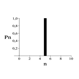
(c) N6

Figure 3: Phonon number distribution exhibiting the creation of Fock state: (a) $|3\rangle$ ($P_{s}^{\prime}=17\%$), (b) $|4\rangle$ ($P_{s}^{\prime}=11\%$), and (c) $|5\rangle$ ($P_{s}^{\prime}=7\%$); all with fidelity of $99\%$ and initial coherent state with $\alpha=0.6$.

In the second strategy, we prepare Fock states $|N\rangle$ with $N=2M$ or $2M-1$. The associated fidelity is also given by the Eq.(18). The Fig.(4) shows the phonon-number distribution exhibiting the creation of Fock states $|3\rangle$, $|4\rangle$, and $|5\rangle$, all them with same fidelity $99\%,$ for an initial coherent state with $\alpha=0.6$.

(a) N4

(b) N5

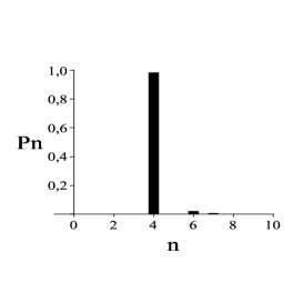
(c) N6

Figure 4: Phonon number distribution exhibiting the creation of Fock state: (a) $|2\rangle$ ($P_{s}^{\prime}=17\%$), (b) $|3\rangle$ ($P_{s}^{\prime}=1\%$), and (c) $|4\rangle$ ($P_{s}^{\prime}=0.3\%$); all with fidelity of $98\%$ and initial coherent state with $\alpha=0.6$.

3 Conclusion

Concerning with the feasibility of the scheme, it is worth mentioning some experimental values of parameters and characteristics of our system: the maximum value of the coupling constant $\beta_{m\acute{a}x}\approx 45MHz$, with $B\approx 0,1T$, $\ell=30\mu m$, $x_{0}=500fm$ and $E_{J}^{0}=5GHz$, with $\omega_{0}=200\pi MHz$. [6, 23, 42, 43, 55, 56, 57, 58, 59]. The expression choosing the time spent to make a hole, $\beta\sqrt{n_{j}+1}\tau_{j}=\pi/2,$ funishes $\tau_{j}\simeq$ $0.3~{}ns,$ when assuming all the CPB previously prepared at $t=0$. On the other hand, the decoherence times of the CPB and the NR are respectively $500~{}ns$ and $160$ $\mu s$ [58]. Accordingly, one may create about 1600 holes before the destructive action of decoherence. However, when considering the success probability to detect all CPB in the state $\left|g\right\rangle$, a more realistic estimation drastically reduces the number of holes. A similar situation occurs in [51, 52, 53], using atom-field system to make holes in the statistical distribution $P_{n}$ of a field state; in this case, about $1\mu s$ is spent to create a hole whereas $1ms$ is the decoherence time of a field state inside the cavity. So, comparing both scenarios the present system is about 60% more efficient in comparison with that using the atom-field system. Concernig with the generation of a Fock state $\left|N\right\rangle$, it is convenient starting with a low excited initial (coherent) state, which involves a low number of Fock components to be deleted via our hole burning procedure. According to the Eq. (18) when one must delete many components of the initial state to achieve the state $\left|N\right\rangle$ this drastically reduces the success probability. As consequence, this method will work only for small values of $N$ ( $N\lesssim 5$ ).

4 Acknowledgements

The authors thank the FAPEG (CV) and the CNPq (ATA, BB) for partially supporting this work.

References

- [1] Bocko M F and Onofrio R, 1996 Rev. Mod. Phys. 68 755
- [2] Munro W J et al. 2002 Phys. Rev. A 66 023819
- [3] Cleland A N and Geller M R 2004 Phys. Rev. Lett. 93 070501
- [4] Cleland A N and Roukes M L 1996 Appl. Phys. Lett. 69 2653
- [5] Carr D W, Evoy S, Sekaric L, Craighead H G and Parpia J M 1999 Appl. Phys. Lett. 75 920
- [6] Huang X M H, Zorman C A, Mehregany M, and Roukes M L 2003 Nature 421 496
- [7] Bose S, Jacobs K and Knight P L 1999 Phys. Rev. A 59 3204
- [8] Midtvedt D, Tarakanov Y and Kinaret J 2011 Nano Lett. 11 1439.
- [9] Knobel R G and Cleland A N 2003 Nature London 424 291
- [10] LaHaye M D , Buu O, Camarota B and Schwab K C 2004 Science 304 74
- [11] Blencowe M 2004 Phys. Rep. 395 159
- [12] Armour A D, Blencowe M P and Schwab K C 2002 Phys. Rev. Lett. 88 148301
- [13] Irish E K and Schwab K 2003 Phys. Rev. B 68 155311
- [14] Santamore D H, Goan H -S, Milburn G J and Roukes M L 2004 Phys. Rev. A 70 052105
- [15] Santamore D H, Doherty A C and Cross M C 2004 Phys. Rev. B 70 144301
- [16] Buks E et al. 2007 arXiv:quant-ph/0610158v4
- [17] Wang Y D, Gao Y B, Sun C P 2004 Eur. Phys. J. B 40 321
- [18] Peano V and Thorwart M 2004 Phys. Rev. B 70 235401
- [19] Takei S, Galitski V M and Osborn K D 2011 arXiv:1104.0029v1
- [20] Liao J Q, Kuang L M 2010 arXiv:1008.1713v1
- [21] Tian L and Zoller P 2004 Phys. Rev. Lett. 93 266403
- [22] Zou X B and Mathis W 2004 Phys. Lett. A 324 484
- [23] Liao J Q, Wu Q Q and Kuang L M 2008 arXiv:0803.4317v1
- [24] Xue F et al. 2007 New J. Phys. 9 35
- [25] Geller M R and Cleland A N 2005 Phys. Rev. A 71 032311
- [26] Tian L and Carr S M 2006 Phys. Rev. B 74 125314
- [27] Wang Y D, Chesi S, Loss D and Bruder C 2010 Phys. Rev. B 81 104524
- [28] Martin I, Shnirman A, Tian L and Zoller P 2004 Phys. Rev. B 69 125339
- [29] Zhang P, Wang Y D and Sun C P 2002 Phys. Rev. Lett. 95 097204
- [30] Wilson-Rae I, Zoller P and Imamoglu A 2004 Phys. Rev. Lett. 92 075507
- [31] Naik A et al. 2006 Nature 443 193
- [32] Hopkins A, Jacobs K, Habib S and Schwab K 2003 Phys. Rev. B 68 235328
- [33] Y.D. Wang et al. 2009 Phys. Rev. B 80 144508
- [34] Hensinger W K et al. 2005 Phys. Rev. A 72 041405
- [35] Sun CP, Wei L F, Liu Y and Nori F 2006 Phys. Rev. A 73 022318
- [36] Milburn G J, Holmes C A, Kettle L M and Goan H S 2007 arXiv:cond-mat/0702512v1
- [37] Siewert J, Brandes T and Falci G 2005 arXiv:cond-mat/0509735v1
- [38] Tian L 2005 Phys. Rev. B 72 195411
- [39] Valverde C, Avelar A T and Baseia B 2011 arXiv:1104.2106v1
- [40] Rabl P, Shnirman A and Zoller P 2004 Phys. Rev. B 70 205304
- [41] Ruskov R, Schwab K and Korotkov A N 2005 Phys. Rev. B 71 235407
- [42] Xue F, Liu Y, Sun C P, Nori F 2007 Phys. Rev. B 76 064305
- [43] Zhou X X and Mizel A 2006 Phys. Rev. Lett. 97 267201
- [44] Suh J et al. 2010 Nano Lett. 10 3990.
- [45] Valverde C, Avelar A T, Baseia B and Malbouisson J M C 2003 Phys. Lett. A 315 213
- [46] Valverde C and Baseia B 2004 Int. J. Quantum Inf. 2 421
- [47] Eisert J, Plenio M B, Bose S and Hartley J 2004 Phys. Rev. Lett. 93 190402
- [48] Bose S and Agarwal G S 2005 New J. Phys. 8 34
- [49] Blais A et al. 2004 Phys. Rev. A 69 062320
- [50] Moerner W E, Lenth W and Bjorklund G C 1988 in: W.E. Moerner (Ed.), Persistent Spectral Hole-Burning: Science and Applications, Springer, Berlin, p. 251
- [51] Malbouisson J M C and Baseia B 2001 Phys. Lett. A 290 214
- [52] Avelar A T and Baseia B 2004 Opt. Comm. 239 281
- [53] Avelar A T and Baseia B 2005 Phys. Rev. A 72 025801
- [54] Escher B M, Avelar A T, Filho T M R and Baseia B 2004 Phys Rev. A 70 025801
- [55] Wallraff A et al. 2005 Phys. Rev. Lett. 95 060501
- [56] Liao J Q and Kuang L M 2007 J. Phys. B: At. Mol. Opt. Phys. 40 1845
- [57] Xue F, Zhong L, Li Y and Sun C P 2007 Phys. Rev. B 75 033407
- [58] Chen G, Chen Z, Yu L and Liang J 2007 Phys. Rev. A. 76 024301
- [59] Liao J Q and Kuang L M 2008 Eur. Phys. J. B 63 79
- [60] Escher B M, Avelar A T and Baseia B 2005 Phys. Rev. A 72 045803
- [61] Aragao A, Avelar A T, Malbouisson J M C and Baseia B 2004 Phys. Lett. A 329 284