Non-invertibility Criteria in Some Heteroscedastic Models

Abstract

In order to calculate the unobserved volatility in conditional heteroscedastic time series models, the natural recursive approximation is very often used. Following Straumann and Mikosch (2006), we will call the model invertible if this approximation (based on true parameter vector) converges to the real volatility. Our main results are necessary and sufficient conditions for invertibility. We will show that the stationary GARCH($p$, $q$) model is always invertible, but certain types of models, such as EGARCH of Nelson (1991) and VGARCH of Engle and Ng (1993) may indeed be non-invertible. Moreover, we will demonstrate it’s possible for the pair (true volatility, approximation) to have a non-degenerate stationary distribution. In such cases, the volatility estimate given by the recursive approximation with the true parameter vector is inconsistent.

Key Words: Conditionally heteroscedastic time series, EGARCH, VGARCH, invertibility, Lyapunov exponent.

Journal Of Economic Literature Clasification: C14, C58.

1 Introduction

Since their introduction in the seminal papers of Engle (1982) and Bollerslev (1986), there has been a remarkable amount of interest in heteroscedastic models coming from researchers in econometrics and statistics and from financial market practitioners. Since then, many other similar models have been introduced to more accurately reflect different qualities of real data. For example, various authors have proposed a vast number of volatility expressions with asymmetries or thresholds, non-stationarities such as unit roots or time-varying parameters, or have considered multidimensional extensions and non-regular time intervals. We refer to two of more recent reviews Andersen et al. (2009) and Francq and Zakoian (2010) which discuss these and other examples and provide the necessary references.

Heteroscedastic models are used to analyze and forecast the unobserved volatility of different financial time series. It is common to construct predictions for current and future volatility values using a natural recursive volatility approximation. Let us recall its definition for a general conditional heteroscedastic model. We define such model as a solution of

$$\begin{split}y_{t}=\sigma_{t}\varepsilon_{t},\\ \sigma^{2}_{t}=H(\theta,y_{t-1},\ldots,y_{t-p},\sigma^{2}_{t-1},\ldots\sigma^{2}_{t-q}),\quad t\in\mathbb{Z},\end{split}$$ (1)

where $\{y_{t}\}$ is the return process, $\{\sigma_{t}\}$ is the volatility process, $H$ is a known function, $p,q\in\mathbb{N}\cup\{0\}$, $\theta$ is the parameter vector taken from a set $\Theta\subseteq\mathbb{R}^{l}$ and $\{\varepsilon_{t}\}$ are i.i.d. random variables on a probability space $(\Omega,\mathcal{F},P)$. More general versions of (1) are of course possible. Assume that $y_{1-p},\ldots,y_{n}$ are observed, fix $s^{2}\in\mathbb{R}^{+}$ and define the recursive volatility approximation by

$$\begin{split}\hat{\sigma}^{2}_{t}(\theta^{\prime})=s^{2},\quad t=1-q,\ldots,0,\\ \hat{\sigma}^{2}_{t}(\theta^{\prime})=H(\theta^{\prime},y_{t-1},\ldots,y_{t-p},\hat{\sigma}^{2}_{t-1}(\theta^{\prime}),\ldots\hat{\sigma}^{2}_{t-q}(\theta^{\prime})),\quad t>0.\end{split}$$

for any $\theta^{\prime}\in\Theta$. The quantity

$$\hat{\sigma}^{2}_{n}(\hat{\theta}_{n})$$ (2)

is often used as an estimate of the volatility value at $n$, where $\hat{\theta}_{n}$ is any consistent estimator of $\theta$. There are other possible definitions of $\hat{\sigma}^{2}_{t}$. For example, Baillie et al. (1996) suggest using the sample mean of $y_{1-p}^{2},\ldots,y_{n}^{2}$ as a starting point instead of $s^{2}$.

In order for approximations (2) to be consistent, it is natural to at least expect that the approximation $\hat{\sigma}^{2}_{t}(\theta)$ (using the true parameter vector) converges to the unobserved value $\sigma^{2}_{t}$:

$$|\hat{\sigma}^{2}_{t}(\theta)-\sigma^{2}_{t}|\stackrel{{\scriptstyle P}}{{\rightarrow}}0,\quad t\to\infty.$$ (3)

To describe models with property (3), we’ll re-use the following definition from Straumann and Mikosch (2006):

Definition 1.1

Assume for all $\theta\in\Theta$ the model (1) has a strictly stationary solution and (3) is true for any initial point $s^{2}$. Then we say the model has the property of invertibility.

Note that many estimator types and tests are very commonly considered under the assumption of invertibility. Indeed, such estimators as the popular quasi-maximum likelihood estimator (QMLE) of Lee and Hansen (1994) and more recent GMM-type robust estimators of Boldin (2000) or minimum distance estimators as in Sorokin (2004) as well as many others are based on residuals $\{y_{t}/\sigma_{t}(\theta^{\prime})\}$. Their asymptotic properties are commonly established assuming convergence of residuals, therefore under invertibility. The same assumption is used for popular tests types such as goodness-of-fit and dimensionality tests (see Francq and Zakoian (2010)) and structural break tests (Boldin (2002), Horvath and Teyssiere (2001)). Therefore, the issue of non-invertibility is key for such procedures. The notable exception are estimators based on autocovariance function such as Whittle estimator applied in Giraitis and Robinson (2000) and Zaffaroni (2008).

For linear time series models such as ARMA the notion of invertibility is classic, see e.g. Brockwell and Davis (1991). For non-linear models, however, there seem to be more than one possible definition. The definition 1.1 is based on that of Granger and Andersen (1978). For detailed discussion and some further references, see Straumann and Mikosch (2006), subsection 3.2. A related definition of invertibility, in particular for bilinear models, was considered previously in Tong (1990). According to Tong’s definition, the model (1) is called invertible if $\varepsilon_{t}$ is a.s. a measurable function of $(\ldots,y_{t-2},y_{t-1},y_{t})$ for any $t\in\mathbb{Z}$. We’ll refer to this notion as global invertibility (this is in contrast to local invertibility, see the next paragraph). Recently, there have been some further results on invertibility of non-linear models. The threshold MA models were investigated in Ling and Tong (2005) and Ling et al. (2007), and non-linear ARMA (NLARMA) models were discussed in Chan and Tong (2009).

The main goal of this paper is to show that some heteroscedastic models (for example, EGARCH of Nelson (1991) and VGARCH of Engle and Ng (1993)) may in general be non-invertible, even if the model has a strictly stationary solution. Moreover, we will provide necessary and sufficient conditions for invertibility for such models. We will demonstrate that if a model is locally invertible (see Definition 2.5 below, also Chan and Tong (2009) for the similar definition), it is also invertible. On the other hand, we’ll prove that under a slightly more restricting condition than a lack of local invertibility the model is also non-invertible. Moreover, we will show that on an extended probability space there exists a random variable $\xi$, independent with $\sigma\{\varepsilon_{t},\;t\geq 0\}$, such that for $s^{2}=\xi$ the process

$$(\sigma^{2}_{t},\hat{\sigma}^{2}_{t}(\theta)),\quad t\geq 0$$

is stationary but

$$P(\sigma^{2}_{t}=\hat{\sigma}^{2}_{t}(\theta))=0,\quad t\geq 0.$$

To the best of our knowledge, this is the first use of the notion of local invertibility in the literature on heteroscedastic models. Its usefulnes is that it’s much easier to check that invertibility itself, this will be discussed below. The used method is general and may be applied to many other heteroscedastic models.

The rest of the paper is organized as follows: in the subsection 2.1 we provide necessary definitions and discuss non-invertibility in more detail. The main results of the paper are given in the section 3. As a fact of independent interest and an illustration of non-invertibility, we provide the results of numerical simulations showing that it is possible to have deterministic chaos (in the sense of Devaney (1989)) in EGARCH in subsection 3.2. Finally, section 4 contains proofs.

2 Prelimiaries

2.1 Stationarity and Invertibility

Let us recall the definition of the GARCH($p$, $q$) model of Bollerslev (1986). It is defined as a solution of particular case of (1) with $l=p+q+1$ and

$$\begin{split}y_{t}=\sigma_{t}\varepsilon_{t},\\ \sigma_{t}^{2}=\alpha_{0}+\alpha_{1}y^{2}_{t-1}+\ldots+\alpha_{p}y^{2}_{t-p}+\beta_{1}\sigma^{2}_{t-1}+\ldots+\beta_{q}\sigma^{2}_{t-q},\quad t\in\mathbb{Z},\end{split}$$ (4)

where

$$\Theta=\{\alpha_{0}>0,\quad\alpha_{i}\geq 0,\;i=1,\ldots,p,\quad\beta_{j}\geq 0,\;j=1,\ldots,q\}.$$

We’ll be interested in the strictly stationary solution of (4). The necessary and sufficient condition for the existence and uniqueness of such a solution was found in Bougerol and Picard (1992b). For simplicity, let’s consider a case $p=q=1$. Then the condition reads

Condition 2.1

$$E\log(\alpha_{1}\varepsilon_{0}^{2}+\beta_{1})<0.$$

Here and in the rest of the paper we denote the natural logarithm $\log$.

It is easy to see that in GARCH($1$, $1$) model strict stationarity implies invertibility. Indeed, Condition 2.1 implies that $\beta_{1}<1$. Then

$$\hat{\sigma}^{2}_{t}(\theta)-\sigma^{2}_{t}=\alpha_{0}+\alpha_{1}y^{2}_{t-1}+\beta_{1}\hat{\sigma}^{2}_{t-1}(\theta)-(\alpha_{0}+\alpha_{1}y^{2}_{t-1}+\beta_{1}\sigma^{2}_{t-1}(\theta))=\beta_{1}(\hat{\sigma}^{2}_{t-1}(\theta)-\sigma^{2}_{t-1}),$$

therefore

$$|\hat{\sigma}^{2}_{t}(\theta)-\sigma^{2}_{t}|\stackrel{{\scriptstyle a.s.}}{{\rightarrow}}0,\quad t\to\infty,$$

implying invertibility. Using the multidimensional version of Condition 2.1, one can check that the same implication is also true for the general GARCH($p$, $q$).

However, the stationarity does not imply invertibility for other heteroscedastic models. Notably, it turns out this relation fails for the EGARCH model of Nelson (1991) and the VGARCH model of Engle and Ng (1993). For simplicity, we’ll consider only 1-dimensional models of those types.

The general model (1) for the 1-dimensional case may be written as

$$\begin{split}y_{t}=\sigma_{t}\varepsilon_{t},\\ \sigma^{2}_{t}=H(\theta,y_{t-1},\sigma^{2}_{t-1}),\quad t\in\mathbb{Z}.\end{split}$$ (5)

Definition 2.1

EGARCH is defined as a solution of

$$\begin{split}y_{t}=\sigma_{t}\varepsilon_{t},\\ \log\sigma_{t}^{2}=\alpha+\gamma|\varepsilon_{t-1}|+\delta\varepsilon_{t-1}+\beta\log\sigma^{2}_{t-1},\quad t\in\mathbb{Z},\end{split}$$ (6)

where $\theta=(\alpha,\beta,\gamma,\delta)$ is the parameter vector and $\{\varepsilon_{t}\}$ are i.i.d.

Definition 2.2

VGARCH is defined as a solution of

$$\begin{split}y_{t}=\sigma_{t}\varepsilon_{t},\\ \sigma_{t}^{2}=\alpha+\gamma(\varepsilon_{t-1}-\delta)^{2}+\beta\sigma^{2}_{t-1},\quad t\in\mathbb{Z},\end{split}$$ (7)

where $\theta=(\alpha,\beta,\gamma,\delta)$ is the parameter vector and $\{\varepsilon_{t}\}$ are i.i.d.

In order to make the models meaningful, we need to enforce certain restriction on parameter values. For EGARCH, we assume that $\gamma\geq|\delta|$ (see Straumann and Mikosch (2006), p. 20 for discussion of why this is reasonable, note somewhat different notation) and that $\beta>0$. For VGARCH, we demand that $\alpha>0,\;\beta>0,\gamma\geq 0$.

It follows from the Theorem 2.5 from Bougerol and Picard (1992a) that a necessary and sufficient conditions for the existence of a strictly stationary solution to (6) and (7) are given by

Condition 2.2

$$E\log\left|\alpha+\gamma|\varepsilon_{0}|+\delta\varepsilon_{0}\right|<\infty,\quad\beta<1.$$

Condition 2.3

$$E\log\left(\alpha+\gamma(\varepsilon_{0}-\delta)^{2}\right)<\infty,\quad\beta<1.$$

respectively. We will assume these conditions to hold throughout the rest of the paper, and denote the stationary solution of either (6) or (7) by $\{\overline{\sigma}_{t}\}$.

The issue of invertibility is, however, more complicated. First, let’s consider the explicit expressions for $\hat{\sigma}^{2}(\theta)$. Since the sequence of random variables $\{\varepsilon_{t}\}$ is unobservable, it needs to be approximated. Commonly this is done using the residuals

$$\hat{\varepsilon}_{t}(\theta^{\prime})=y_{t}/\hat{\sigma}_{t}(\theta^{\prime})$$

For EGARCH, we define $\hat{\sigma}^{2}(\theta^{\prime})$ recursively as a solution of

$$\begin{split}\log\hat{\sigma}^{2}_{t}(\theta^{\prime})=s^{2},\quad t=0,\\ \log\hat{\sigma}^{2}_{t}(\theta^{\prime})=\alpha^{\prime}+\beta^{\prime}\log\hat{\sigma}^{2}_{t-1}(\theta^{\prime})+\gamma^{\prime}|\hat{\varepsilon}_{t-1}(\theta^{\prime})|+\delta^{\prime}\hat{\varepsilon}_{t-1}(\theta^{\prime}),\quad t>0.\end{split}$$ (8)

For VGARCH $\hat{\sigma}^{2}(\theta^{\prime})$ are given by

$$\begin{split}\log\hat{\sigma}^{2}_{t}(\theta^{\prime})=s^{2},\quad t=0,\\ \hat{\sigma}^{2}_{t}(\theta^{\prime})=\alpha^{\prime}+\beta^{\prime}\hat{\sigma}^{2}_{t-1}(\theta^{\prime})+\gamma^{\prime}(\hat{\varepsilon}_{t-1}(\theta^{\prime})-\delta^{\prime})^{2},\quad t>0.\end{split}$$ (9)

In both cases, we have

$$\hat{\sigma}^{2}_{t}(\theta^{\prime})=f_{t-1}(\hat{\sigma}^{2}_{t-1}(\theta^{\prime})),\quad t>0,$$

where $\{f_{t}(\cdot)\}$ is a sequence of random transformations $\mathbb{R}^{+}\to\mathbb{R}^{+}$, defined for the general model (5) by

$$f_{t}(x)=H(\theta,y_{t},x),\quad t\in\mathbb{Z},\;x\in\mathbb{R}^{+}.$$

Crucially, the random transformations defining $\{\sigma^{2}_{t}\}$ (cf. (6), (7)) and those defining $\{\hat{\sigma}^{2}_{t}(\theta)\}$ (cf. (8), (9)) are different. Indeed, for the general model (5) we have

$$\begin{cases}\sigma^{2}_{t}=H(\theta,\sigma_{t-1}\varepsilon_{t-1},\sigma^{2}_{t-1}),\\ \hat{\sigma}^{2}_{t}(\theta)=H(\theta,\sigma_{t-1}\varepsilon_{t-1},\hat{\sigma}^{2}_{t-1}(\theta))\end{cases}\quad t\geq 1.$$ (10)

Note that the right-hand side of the second equation in (10) depends not only on $\hat{\sigma}^{2}_{t-1}(\theta)$, but also on $\sigma^{2}_{t-1}$.

For a general heteroscedastic model invertibility holds if the top Lyapunov exponent of the corresponding sequence $\{f_{t}(\cdot)\}$ is negative (Proposition 3.7 of Straumann and Mikosch (2006)). Let us recall the definition of Lyapunov exponent of a family of transformations:

Definition 2.3

Assume $\{f_{t}(\cdot)\}_{t\in\mathbb{Z}}$ is a stationary ergodic family of $\mathbb{R}\to\mathbb{R}$ functions, such that

$$E\log\Lambda(f_{t})<\infty,$$

where $\Lambda$ is the Lipchitz norm,

$$\Lambda(f):=\sup_{x\neq y}\frac{|f(x)-f(y)|}{|x-y|}.$$

Then the quantity

$$\lambda=\inf\left\{E\left(\frac{1}{t+1}\log\Lambda(f_{t}\circ\ldots\circ f_{0})\right),t\in\mathbb{N}\right\}$$

is called the top Lyapunov exponent.

However, estimating top Lyapunov exponent for nonlinear systems is not straightforward (and therefore checking whether the sufficient condition for invertibility holds is hard, p. 21 of Straumann and Mikosch (2006)). Note that the second equation of (10) could be nonlinear in $\hat{\sigma}^{2}_{t-1}(\theta)$ even if the first one is linear! Therefore, the results of Bougerol and Picard (1992a) are not applicable. To the best of our knowledge, necessary and sufficient conditions for invertibility of such nonlinear models are not known.

We will consider a simple lower bound for the Lyapunov exponent which will be useful for the construction of a criteria for invertibility. From now on, we will write $\hat{\sigma}^{2}_{t}$ instead of $\hat{\sigma}^{2}_{t}(\theta)$ for brevity.

Definition 2.4

Assume that the equation (5) has a unique stationary solution $\{\overline{\sigma}^{2}_{t}\}_{t\in\mathbb{Z}}$. Assume also that for any fixed $\theta\in\Theta$ the function $H(\theta,\cdot,\cdot)$ is continuously differentiable. Denote

$$\Lambda^{y}_{t}=\left|\left.\frac{\partial}{\partial\hat{\sigma}^{2}_{0}}\right|_{\hat{\sigma}^{2}_{0}=\overline{\sigma}^{2}_{0}}(f_{t}\circ\ldots\circ f_{0})\right|,$$

$$\lambda^{y}=\inf\left\{E\left(\frac{1}{t+1}\log\Lambda^{y}_{t}\right),t\in\mathbb{N}\right\}.$$

We will refer to $\lambda^{y}$ as stability coefficient and call a heteroscedastic model locally invertible if $\lambda^{y}<0$ and locally non-invertible otherwise.

A similar definition for non-linear ARMA models was considered in Chan and Tong (2009).

Unlike top Lyapunov exponent, $\lambda^{y}$ may be written down explicitly using the chain differentiation rule. Denote

$$H^{\prime}_{x}(\theta,y,x)=\frac{\partial H(\theta,y,x)}{\partial x},$$

then

$$\Lambda^{y}_{t}=\left|\left.\frac{\partial}{\partial\hat{\sigma}^{2}_{0}}\right|_{\hat{\sigma}^{2}_{0}=\overline{\sigma}^{2}_{0}}(f_{t}\circ\ldots\circ f_{0})\right|=\prod_{k=0}^{t}\left|H^{\prime}_{x}(\theta,\overline{\sigma}_{k}\varepsilon_{k},\overline{\sigma}^{2}_{k})\right|,$$

therefore

$$\log\Lambda^{y}_{t}=\sum_{k=0}^{t}\log\left|H^{\prime}_{x}(\theta,\overline{\sigma}_{k}\varepsilon_{k},\overline{\sigma}^{2}_{k})\right|.$$

If the process $\{\overline{\sigma}^{2}_{t}\}$ is ergodic and

$$E\log\left|H^{\prime}_{x}(\theta,\overline{\sigma}_{0}\varepsilon_{0},\overline{\sigma}^{2}_{0})\right|<\infty,$$

due to Birkhoff-Khinchin ergodic theorem

$$\lambda^{y}=E\log\left|H^{\prime}_{x}(\theta,\overline{\sigma}_{0}\varepsilon_{0},\overline{\sigma}^{2}_{0})\right|.$$ (11)

Also note that since

$$\Lambda^{y}_{t}\leq\Lambda(f_{t}\circ\ldots\circ f_{0}),$$

it must also be that

$$\lambda^{y}\leq\lambda.$$

The quantity $\lambda^{y}$ has an intuitive interpretation. It indicates whether the behaviour of $\hat{\sigma}^{2}_{t}$ is convergent or explosive in the neighborhood of the true volatility value $\sigma^{2}_{t}$ (this will be formalized in Theorems 3.1 - 3.4). For the invertibility of (5), three cases are possible:

1. If $\lambda^{y}\leq\lambda<0$, $\hat{\sigma}^{2}_{t}$ is stable and invertibility takes place (see Straumann and Mikosch (2006), Theorem 2.8).

2. If $\lambda^{y}\leq 0\leq\lambda$, Theorem 2.8 of Straumann and Mikosch (2006) is not valid anymore. The behaviour of $\hat{\sigma}^{2}_{t}$ is ”stable” in the neighborhood of the true volatility value $\sigma^{2}_{t}$.

3. If $0<\lambda^{y}\leq\lambda$, the behaviour of $\hat{\sigma}^{2}_{t}$ is explosive in the neighborhood of the true volatility value $\sigma^{2}_{t}$.

Definition 2.5

Assume that the system (10) has a stationary solution $(\overline{\sigma}^{2}_{t},\hat{\overline{\sigma}}^{2}_{t})_{t\geq 0}$ on an extended probability space such that

$$P(\overline{\sigma}^{2}_{0}=\hat{\overline{\sigma}}^{2}_{0})=0,\quad\geq 0.$$

Then we call the model (5) properly non-invertible.

It is interesting that the unstable assumption of case 3 is (under mild technical conditions) sufficient for the proper non-invertibility for EGARCH and VGARCH models. On the other hand, in case 2 if we only assume that $\lambda^{y}<0$, both models are invertible. These are the main results of this paper, to be considered in the following section. In addition, we show that in both cases for any starting point $s^{2}$ the sample distribution of

$$(\sigma^{2}_{t},\hat{\sigma}^{2}_{t}),\quad t=0,\ldots,n$$

converges to the stationary one. Together with proper non-invertibility it implies that the approximation $\hat{\sigma}^{2}_{t}$ is inconsistent if $\lambda^{y}>0$.

3 Main Results

Before we formulate the main results, let’s introduce the conditions to be used. First one is a regularity condition.

Condition 3.1

The distribution of $\varepsilon_{0}$ is absolutely continuous with respect to Lebesgue measure on $\mathbb{R}$ with continuous density $g(x)$, $E\varepsilon_{0}=0$, $E\varepsilon_{0}^{2}=1$ and

$$g(x)>0\;\forall x\in\mathbb{R},\qquad\sup_{x\in\mathbb{R}}(|x|+1)g(x)<\infty.$$

Condition 3.1 may probably be somewhat relaxed, although a condition similar to $g(x)>0$ is essential in establishing the $\psi$-irreducibility of relevant Markov chains, see Proofs section.

We will formulate the assumption on $\lambda^{y}$ using the equation (11). Denote $\lambda^{y}_{E}$ and $\lambda^{y}_{V}$ stability coefficients for EGARCH and VGARCH respectively. Note that for EGARCH due to (8)

$$H^{E}(\theta,y,x)=\exp\left\{\alpha+\beta\log x+(\gamma|y|+\delta y)x^{-1/2}\right\},\quad\left(H^{E}\right)^{\prime}_{x}(\theta,y,x)=H^{E}(\theta,y,x)\left(\beta x^{-1}-(\gamma|y|+\delta y)x^{-3/2}/2\right),$$

and by definition of the stationary solution $\overline{\sigma}_{t}$

$$\lambda^{y}_{E}=E\log\left|H^{E}(\theta,\overline{\sigma}_{0}\varepsilon_{0},\overline{\sigma}^{2}_{0})\right|-E\log|\overline{\sigma}^{2}_{0}|+E\log\left|\beta-(\gamma|\overline{\sigma}_{0}\varepsilon_{0}|+\delta\overline{\sigma}_{0}\varepsilon_{0})\overline{\sigma}^{-1}_{0}/2\right|=$$

$$E\log\left|\beta-2^{-1}(\gamma|\varepsilon_{0}|+\delta\varepsilon_{0})\right|.$$

For VGARCH due to (9)

$$H^{V}(\theta,y,x)=\alpha+\beta x+\gamma(yx^{-1/2}-\delta)^{2},\quad\left(H^{V}\right)^{\prime}_{x}(\theta,y,x)=\beta-\gamma yx^{-3/2}(yx^{-1/2}-\delta)$$

and

$$\lambda^{y}_{V}=E\log\left|\beta-\gamma\overline{\sigma}_{0}\varepsilon_{0}\overline{\sigma}_{0}^{-3}(\overline{\sigma}_{0}\varepsilon_{0}\overline{\sigma}_{0}^{-1}-\delta)\right|=E\log\left|\beta-\gamma\varepsilon_{0}\overline{\sigma}_{0}^{-2}(\varepsilon_{0}-\delta)\right|.$$

3.1 Invertibility criteria

Now we will formulate the main results:

Theorem 3.1 (Proper non-invertibility for EGARCH)

Assume the Conditions 2.2 and 3.1 hold and $\lambda^{y}_{E}>0$. Then the system (10) with $H=H^{E}$ has a stationary solution $\{(\overline{\sigma}^{2}_{t},\hat{\overline{\sigma}}^{2}_{t})\}_{t\geq 0}$ on an extended probability space such that

$$P(\overline{\sigma}^{2}_{0}=\hat{\overline{\sigma}}^{2}_{0})=0.$$

Theorem 3.2 (Proper non-invertibility for VGARCH)

Assume the Conditions 2.3 and 3.1 hold and $\lambda^{y}_{V}>0$. Then the system (10) with $H=H^{V}$ has a stationary solution $\{(\overline{\sigma}^{2}_{t},\hat{\overline{\sigma}}^{2}_{t})\}_{t\geq 0}$ on an extended probability space such that

$$P(\overline{\sigma}^{2}_{0}=\hat{\overline{\sigma}}^{2}_{0})=0.$$

Besides the proper non-invertibility, another important question is the joint behaviour of the true volatility $\sigma^{2}_{t}$ and its approximation $\hat{\sigma}^{2}_{t}$. As it turns out, the sample distribution converges to the stationary one:

Theorem 3.3 (LLN for $\{(\sigma^{2}_{t},\hat{\sigma}^{2}_{t})\}$ in EGARCH)

Assume the conditions 2.2 and 3.1 are fulfilled.

i) If $\lambda^{y}_{E}>0$, the process $\{(\overline{\sigma}^{2}_{t},\hat{\overline{\sigma}}^{2}_{t})\}$, the stationary solution of (10) with $H=H_{E}$, is ergodic and for any $B\in\mathcal{B}(\mathbb{R}^{2})$ and starting point $s^{2}$

$$n^{-1}\sum_{t=0}^{n-1}I\{(\sigma^{2}_{t},\hat{\sigma}^{2}_{t})\in B\}\stackrel{{\scriptstyle a.s.}}{{\rightarrow}}P((\overline{\sigma}^{2}_{0},\hat{\overline{\sigma}}^{2}_{0})\in B),\quad n\to\infty,$$

where $I\{\cdot\}$ is the indicator function.

ii) If $\lambda^{y}_{E}<0$, for any starting point $s^{2}$ and $\mu>0$

$$P(|\sigma^{2}_{0}-\hat{\sigma}^{2}_{0}|\geq\mu)\to 0.$$

Theorem 3.4 (LLN for $\{(\sigma^{2}_{t},\hat{\sigma}^{2}_{t})\}$ in VGARCH)

Assume the conditions 2.2 and 3.1 are fulfilled.

i) If $\lambda^{y}_{V}>0$, the process $\{(\overline{\sigma}^{2}_{t},\hat{\overline{\sigma}}^{2}_{t})\}$, the stationary solution of (10) with $H=H_{V}$, is ergodic and for any $B\in\mathcal{B}(\mathbb{R}^{2})$ and starting point $s^{2}$

$$n^{-1}\sum_{t=0}^{n-1}I\{(\sigma^{2}_{t},\hat{\sigma}^{2}_{t})\in B\}\stackrel{{\scriptstyle a.s.}}{{\rightarrow}}P((\overline{\sigma}^{2}_{0},\hat{\overline{\sigma}}^{2}_{0})\in B),\quad n\to\infty.$$

ii) If $\lambda^{y}_{V}<0$, for any starting point $s^{2}$ and $\mu>0$

$$P(|\sigma^{2}_{0}-\hat{\sigma}^{2}_{0}|\geq\mu)\to 0.$$

Theorems 3.1 - 3.4 indicate that for some parameter vectors finite sample volatility approximations do not converge to the actual volatility as the sample size increases. In particular, the standard recursive volatility estimator is inconsistent (this is easily checked by setting

$$B=\{(\sigma^{2},\hat{\sigma}^{2})\in\mathbb{R}^{2}_{+}:|\sigma^{2}-\hat{\sigma}^{2}|\geq\mu\}$$

for a $\mu>0$ and applying Theorems 3.3 and 3.4).

The general heteroscedastic model (5) considered in this paper can be re-written as a particular case of NLARMA model (see Chan and Tong (2009), Equation (3)). The issue of invertibility then also becomes a special case of invertibility of NLARMA. However, the latter paper discusses only local invertibility for such models. Therefore, our results complement Chan and Tong (2009) since we establish that local invertibility is (except the case $\lambda^{y}=0$ ) equivalent to invertibility for particular cases of NLARMA. It would be very interesting to investigate global invertibility of heteroscedastic models such as EGARCH and VGARCH. It easy to see that a stationary invertible model is necessary globally invertible. Indeed, denote for any $t\in\mathbb{Z}$, $k\geq 1$

$$\hat{\sigma}^{2}_{t,k,s^{2}}=H(\theta,y_{t-1},H(\theta,y_{t-2},\ldots H(\theta,y_{t-k},s^{2})\ldots),$$

so that $\hat{\sigma}^{2}_{t}=\hat{\sigma}^{2}_{t,t,s^{2}}$. Then due to invertibility

$$\hat{\sigma}^{2}_{t,k,s^{2}}\stackrel{{\scriptstyle P}}{{\to}}\sigma_{t}^{2}$$

as $k\to\infty$ and for some sub-sequence $\{k_{n}\}$

$$\hat{\sigma}^{2}_{t,k_{n},s^{2}}\stackrel{{\scriptstyle a.s.}}{{\to}}\sigma_{t}^{2}$$

as $n\to\infty$. The reverse relation seems more complicated and is left for future research.

Another problem (which also will not be considered here) is the behaviour of tests and estimates unver non-invertibility. Commonly, consistency and asymptotic normalilty are established under invertibility assumption. However, it was shown in Zaffaroni (2008) that the Whittle estimator (which is not residual-based) remains asymptotically normal under non-invertibility too. It will be interesting to see what happens to common estimators such as QMLE.

Finally, it is possible in principle that the conditions ensuring the existence of the stationary solution and the lack of stability are mutually exclusive and therefore the Theorems 3.1 - 3.4 are vacuous. However, it is easy to check the opposite (see also the Figures 3.1 and 3.2).

For EGARCH, we’ll show that for any distribution of $\{\varepsilon_{0}\}$ satisfying Condition 3.1 there exists $\theta$, such that the Condition 2.2 is satisfied and $\lambda^{y}_{E}>0$. Indeed, the Condition 2.2 is satisfied if $\beta<1$ and $E|\log|\varepsilon_{0}||<\infty$. Condition 3.1 ensures that the latter holds. It therefore suffices to choose arbitrary $\alpha>0$, $\beta<1$, $\delta=0$ and large enough $\gamma$.

For VGARCH we’ll only check a more relaxed statement. Assume in addition to Condition 3.1 that there exists $\mu\in\mathbb{R}$, such that

$$E\log|\varepsilon_{0}-\mu|<E\log|\varepsilon_{0}|.$$

As a particular example of a distribution with such property, it suffices to choose a unimodal non-symmetric distribution with a maximum not at $0$. For example, an appropriately scaled mixture of $\xi_{1}$ and $-\xi_{2}$, where both $\xi_{1}$ and $\xi_{2}$ had exponential distributions but with different parameters, is one such distribution.

Put $\beta=0$ and select arbitrary $\gamma>0$, $\alpha>0$ and $\delta=\mu$. Then

$$\overline{\sigma}^{2}_{0}=\alpha+\gamma(\varepsilon_{-1}-\mu)^{2},\quad\left(H^{V}\right)^{\prime}_{x}(\theta,\overline{\sigma}_{0}\varepsilon_{0},\overline{\sigma}^{2}_{0})=\frac{\gamma\varepsilon_{0}(\varepsilon_{0}-\mu)}{\alpha+\gamma(\varepsilon_{-1}-\mu)^{2}}.$$

Due to dominated convergence theorem, when $\alpha\to 0+$,

$$E\log\left|\beta-\gamma\varepsilon_{0}\overline{\sigma}^{-2}_{0}(\varepsilon_{0}-\mu)\right|=E\log\left|\frac{\gamma\varepsilon_{0}(\varepsilon_{0}-\mu)}{\alpha+\gamma(\varepsilon_{-1}-\mu)^{2}}\right|\to$$

$$E\log\left|\frac{\varepsilon_{0}}{\varepsilon_{-1}-\mu}\right|=E\log|\varepsilon_{0}|-E\log|\varepsilon_{-1}-\mu|>0.$$

For arbitrary $\gamma$ and $\alpha$ and $\beta$ small enough, $\lambda^{y}_{V}>0$.

To illustrate the main results, we show the figures demonstrating the behaviour of instability coefficient $\lambda^{y}$ and sample paths of models (6) and (7).

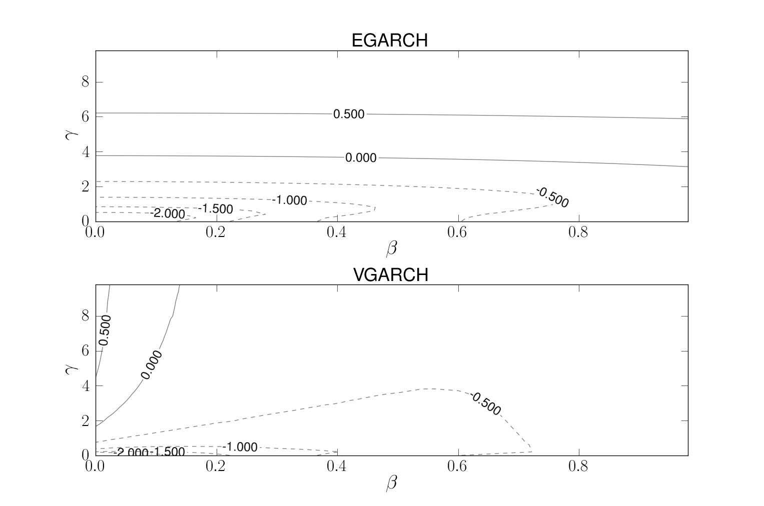
Figure 3.1: Heatmap of $\lambda^{y}_{E}$ and $\lambda^{y}_{V}$. Positive values correspond to non-invertible models. For EGARCH, we used $\alpha=0.1$, $\beta=0.25$, $\gamma=5.4$ and standard normal $\varepsilon_{1}$. For VGARCH, we used $\alpha=0.001$, $\beta=0.01$, $\delta=-0.3$, $\gamma=1$ and $\varepsilon_{1}$ was an appropriately scaled mixture of $\xi_{1}$ and $-\xi_{2}$, where both $\xi_{1}$ and $\xi_{2}$ had exponential distributions with parameters $1$ and $4$.

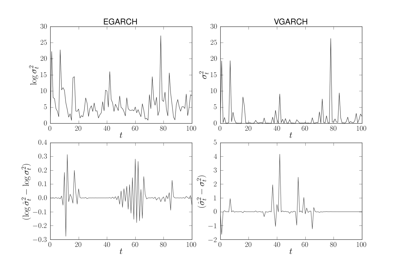
Figure 3.2: EGARCH and VGARCH simulation results. The top plot shows simulated $\sigma^{2}_{t}$ as a function of $t$. The bottom plot shows the difference $(\hat{\sigma}^{2}_{t}-\sigma^{2}_{t})$ as a function of $t$.

3.2 Deterministic Chaos in EGARCH

We’ll discuss a simple case of deterministic EGARCH model, which sheds light onto the origin of non-invertibility in this particular model and also on the intuitive sense of local invertibility. Assume that the Condition 2.2 is satisfied and

$$P(\varepsilon_{1}=1)=P(\varepsilon_{1}=-1)=1/2,\quad\beta<1,\quad\delta=0,$$ (12)

then

$$\log\overline{\sigma}_{t}^{2}\equiv\log\overline{\sigma}^{2}=(\alpha+\gamma)/(1-\beta),$$

$$d_{t}=f(d_{t-1}),\quad f(x)=\alpha+\beta x+\gamma e^{-d_{t-1}/2},\quad d_{t}=\log\hat{\sigma}_{t}^{2}-\log\sigma_{t}^{2},\quad t\in\mathbb{Z}.$$ (13)

We don’t pursue the task of the formal proof, but numerical simulations show that the dynamical system given by $f$ of (13) is chaotic in the sense of Devaney once $\gamma$ is large enough. More precisely, when $\gamma$ increases, the system experiences period-doubling bifurcations and eventually becomes chaotic.

The bifurcation diagram of (13) is shown at Figure 3.3.

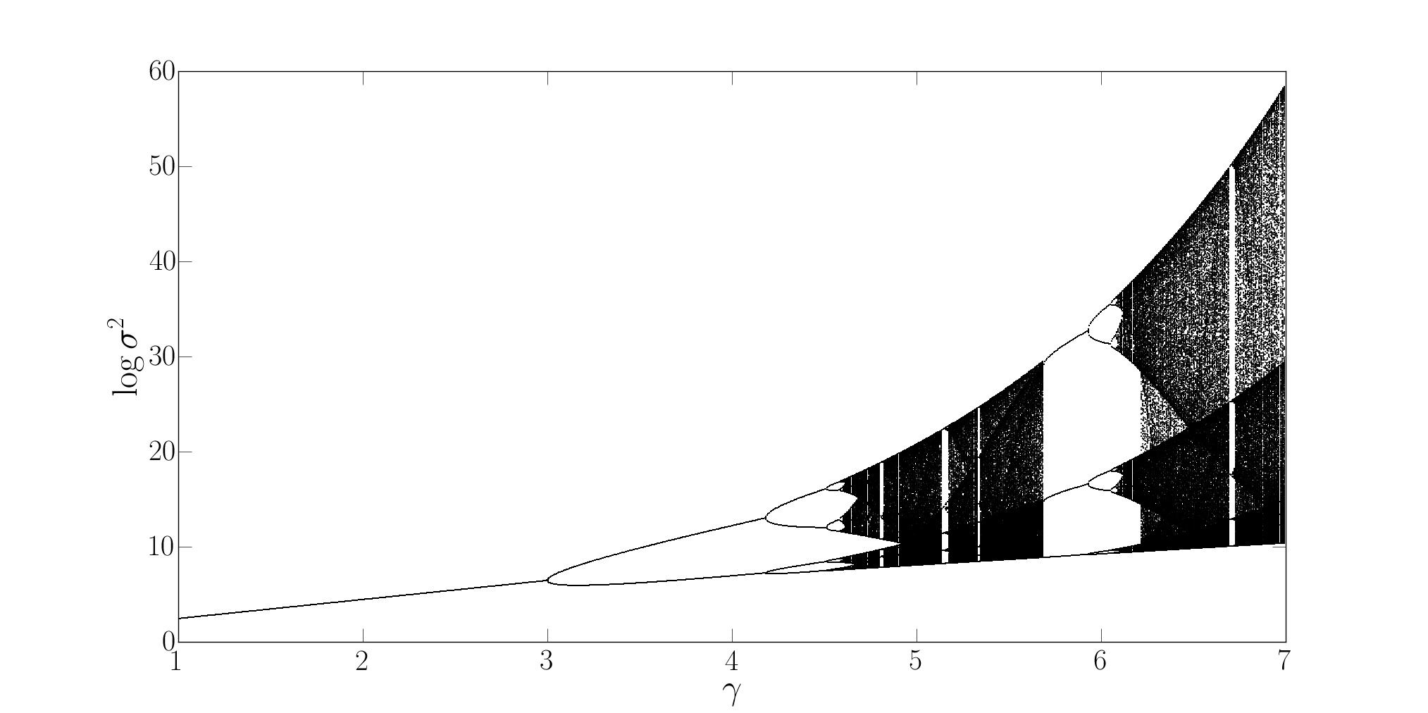
Figure 3.3: Deterministic EGARCH bifurcation diagram for $\alpha=0.2$, $\beta=0.5$.

As discussed in Devaney (1989), the period-doubling behaviour is typical for maps $\mathbb{R}\to\mathbb{R}$. For example, the famous logistic map $x\mapsto\gamma x(1-x)$ exhibits the same type of bifurcations. It is also quite interesting that under (12) the local non-invertibility of EGARCH is equivalent to instability of $\log\overline{\sigma}^{2}$ which is the only fixed point of $f$. If this point was stable in the sense of $\lambda^{y}_{E}<0$, there would be at least an interval of stable behaviour. In the general ”stochastic” case, discussed in the previous subsection, the stability is equivalent to invertibility with the exception of the case $\lambda^{y}=0$.

4 Proofs

4.1 Markov chain foundations

In this section, we’ll present the proofs of Theorems 3.1 - 3.4. The main technical tool used is the general result stating the existence of a stationary distribution in Markov chains (Theorem 10.0.1 of Meyn and Tweedie (2009)), we’ll re-state it for convenience. We also re-use some notation and definitions from the book.

Assume that $\{\Phi_{t}\}_{t\in\mathbb{Z}}$ is a Markov chain with a polish space $\mathcal{X}$ as state space, transition probabilitites $P(x,A),\;x\in\mathcal{X},\;A\in\mathcal{B}(\mathcal{X})$, $\phi$ is a measure on $\mathcal{B}(\mathcal{X})$. Also fix $\{a_{i}\}$ - a distribution on $\mathbb{N}^{+}$. Denote

$$\tau_{A}=\inf\{t\geq 0:\Phi_{t}\in A\},\quad\eta_{A}=\sum_{t\geq 1}I\{\Phi_{t}\in A\},$$

$$P_{x}(\cdot)=P(\cdot|\Phi_{0}=x),\quad E_{x}[\cdot]=E[\cdot|\Phi_{0}=x].$$

$$L(x,A)=P_{x}(\tau_{A}<\infty).$$

Denote $\psi$ the maximal irreducibility measure (see (Meyn and Tweedie, 2009, Proposition 4.2.2)),

$$\mathcal{B}^{+}(\mathcal{X})=\{B\in\mathcal{B}(\mathcal{X}):\psi(B)>0\}.$$

Theorem 4.1 (Theorem 10.0.1 of Meyn and Tweedie (2009))

If the chain $\Phi$ is recurrent then it admits a unique (up to constant multiples) invariant measure $\pi$. This invariant measure is finite (rather than merely $\sigma$-finite, and therefore the chain is positive), if there exists a petite set $C$ such that

$$\sup_{x\in C}E_{x}[\tau_{C}]<\infty.$$ (14)

4.2 Proofs of Theorems 3.1 and 3.2

The proofs of these two theorems will follow exactly the same recipe. In Step 1, we establish the following drift criteria from Meyn and Tweedie (2009) for a certain set $C$:

Definition 4.1 (Strict drift towards C)

For some set $C\in\mathcal{B}(\mathcal{X})$, some constants $b<\infty$ and $\mu>0$ and an extended real-valued function $V:\mathcal{X}\to[0,\infty]$

$$\Delta V(x)\leq-\mu I\{x\notin C\}+bI\{x\in C\},\quad x\in\mathcal{X},$$ (15)

where

$$\Delta V(x)=E_{x}[V(\Phi_{1})]-V(x),\quad x\in\mathcal{X}.$$

In Step 2 we’ll check that the chosen $C$ is petite.

In Step 3 we check the condition (14) and $\psi$-irreducibility of $\{\Phi_{t}\}$, using the strict drift condition.

Finally, we establish that the appropriate Markov chain is indeed recurrent using the following slightly modified version of Theorem 8.4.3 from Meyn and Tweedie (2009):

Theorem 4.2

Assume that $\{\Phi_{t}\}$ is $\psi$-irreducible and there exist a petite set $C$ and a function $V$ which is unbounded off petite sets (in the sense that $C_{V}(n)=\{y:V(y)\leq n\}$ is petite for all n), such that $\Phi$ has a strict drift towards $C$. Then $L(x,C)=1$ for all $x\in\mathcal{X}$ and $\Phi$ is recurrent.

The recurrence of $\{\Phi_{t}\}$ and Theorem 4.1 imply the existence of the stationary distribution $\pi$, and finally the equation (14) ensures $\pi$ is finite.

Throughout the proofs we will denote $o_{B}(1)$ ($O_{B}(1)$) a function of $B$ which converges to $0$ (is bounded) as $B\to\infty$ and model parameters and the distribution of $\varepsilon_{0}$ are fixed.

Proof of Theorem 3.1.

First of all, note that the equation (8) together with (6) are equivalent to

$$\begin{cases}z_{t}=\alpha+\beta z_{t-1}+\gamma|\varepsilon_{t-1}|+\delta\varepsilon_{t-1},\\ \hat{z}_{t}=\alpha+\beta\hat{z}_{t-1}+(\gamma|\varepsilon_{t-1}|+\delta\varepsilon_{t-1})\exp\{-d_{t-1}/2\},\end{cases}\quad t\geq 1,$$ (16)

where we define

$$z_{t}=\log\sigma^{2}_{t},\quad\hat{z}_{t}=\log\hat{\sigma}^{2}_{t}(\theta),\quad d_{t}=\hat{z}_{t}-z_{t},\quad t\geq 0.$$

It is more convenient to instead consider the chain $\{(z_{t},d_{t})\}$ defined by

$$\begin{cases}z_{t}=\alpha+\beta z_{t-1}+\varepsilon^{*}_{t-1},\\ d_{t}=\beta d_{t-1}+\varepsilon^{*}_{t-1}(\exp\{-d_{t-1}/2\}-1),\end{cases}\quad t\geq 1,$$ (17)

where for brevity we put

$$\varepsilon^{*}_{t}=\gamma|\varepsilon_{t}|+\delta\varepsilon_{t},\quad t\geq 0,$$

denote for $x\in\mathbb{R}$

$$e_{x}=\exp\{-x/2\}-1,\quad x^{+}=\max(x,0)$$

and recursively define

$$h_{1}(z,x)=\alpha+\beta z+x,\quad h_{t}(z,x_{1},\ldots,x_{t})=h_{1}(h_{t-1}(z,x_{1},\ldots,x_{t-1}),x_{t}),\quad t\geq 2,$$

$$\hat{h}_{1}(d,x)=\beta d+xe_{d},\quad\hat{h}_{t}(d,x_{1},\ldots,x_{t})=\hat{h}_{1}(\hat{h}_{t-1}(d,x_{1},\ldots,x_{t-1}),x_{t}),\quad t\geq 2,$$

so that

$$z_{t}=h_{t}(z_{0},\varepsilon^{*}_{0},\ldots,\varepsilon^{*}_{t-1}),\quad d_{t}=\hat{h}_{t}(d_{0},\varepsilon^{*}_{0},\ldots,\varepsilon^{*}_{t-1}).$$

It is easy to see that for any $d\neq 0$ and $t\geq 0$ under Condition 3.1 $P_{(z,d)}(d_{t}=0)=0$. Indeed, due to Condition 3.1 $P(\varepsilon^{*}_{0}=x)=0$ for any $x\neq 0$ and

$$P_{(z,d)}(d_{1}=0)=P_{(z,d)}\Bigl{(}\beta d_{0}+\varepsilon^{*}_{0}e_{d}=0\Bigr{)}=P_{(z,d)}\Bigl{(}\varepsilon^{*}_{0}=-\beta d_{0}e_{d}^{-1}\Bigr{)}=0.$$

For an arbitrary $t\geq 0$ we get the result by induction and Fubini theorem. From now on we will consider the modification of the chain $\{(z_{t},d_{t})\}$ on the space

$$\mathcal{X}_{E}=\mathbb{R}\times(\mathbb{R}\backslash\{0\})$$

(which exists as we’ve just shown).

Step 1. Put for some $k>0$

$$V_{E}(z,d)=R(d)+k|z|,\quad R(d)=\begin{cases}-d-1,&\mbox{if }d<-1\\ -\log|d|,&\mbox{if }|d|\leq 1\\ \log d,&\mbox{if }d>1\end{cases},$$

$$C_{E}(A,B)=\left\{(z,d)\in\mathcal{X}_{E}:0\leq|z|\leq A,|d|\geq B^{-1},|d|\leq B\right\}.$$

We’ll first show that for some $\mu>0$ and all $(z,d)\in\mathcal{X}_{E}\backslash C_{E}(A,B)$

$$E_{(z,d)}[V_{E}(z_{1},d_{1})]\leq V_{E}(z,d)-\mu$$ (18)

if $A$ and $B$ are large enough. Indeed,

$$E_{z}|z_{1}|\leq|\alpha|+\beta|z|+E|\varepsilon^{*}_{0}|\leq O_{B}(1)+\beta|z|.$$ (19)

Note that the conditions $\lambda^{y}_{E}>0$ and $\gamma\geq|\delta|$ ensure that $\gamma>0$. For $d\geq B$ and $B\geq\beta^{-1}$, by the definition of $R$ and Lemma 4.1 (a)

$$E_{d}R(d_{1})=E\log(\beta d+\varepsilon^{*}_{0}e_{d})I\left\{d_{1}\geq 1\right\}+$$

$$E\bigl{[}-\log\left|\beta d+\varepsilon^{*}_{0}e_{d}\right|\bigr{]}I\left\{|d_{1}|<1\right\}+$$

$$E\left(-\beta d-\varepsilon^{*}_{0}e_{d}-1\right)I\left\{d_{1}\leq-1\right\}\leq$$

$$P(d_{1}\geq 1)\log(\beta d)+o_{B}(1)+O_{B}(1)E\varepsilon^{*}_{0}P(d_{1}<-1)\leq\log d+\log\beta+o_{B}(1).$$ (20)

For $d\leq-B$, once again using definition of $R$ and Lemma 4.1 (b), we get

$$E_{d}R(d_{1})=E\bigl{(}-\beta d-\varepsilon^{*}_{0}e_{d}-1\bigr{)}I\left\{d_{1}\leq-1\right\}+$$

$$E\Bigl{[}-\log\bigl{|}\beta d+\varepsilon^{*}_{0}e_{d}\bigr{|}\Bigr{]}I\left\{|d_{1}|<1\right\}+$$

$$E\log\bigl{(}\beta d+\varepsilon^{*}_{0}e_{d}\bigr{)}I\left\{d_{1}\geq 1\right\}\leq$$

$$-\beta dP\left\{d_{1}\leq-1\right\}+\log(-\beta d)P(|d_{1}|<1)+\log(\exp\{-d/2\})+E\log^{+}(\varepsilon^{*}_{1})+O_{B}(1)\leq$$

$$-d/2+O_{B}(1).$$ (21)

For $d\in(0,B^{-1})$, using Taylor’s expansion we find that for any $\rho>0$

$$E_{d}R(d_{1})\leq E\bigl{(}-\beta d-\varepsilon_{0}e_{d}-1\bigr{)}I\left\{d_{1}\leq-1\right\}+$$

$$E\Bigl{|}\log\bigl{|}\beta d+\varepsilon^{*}_{0}e_{d}\bigr{|}\Bigr{|}\leq$$

$$\leq(-e_{d})E\varepsilon^{*}_{0}-\log d+\sup_{x\in(1-\rho,1+\rho)}E\left|\log\left|\beta-x2^{-1}\varepsilon^{*}_{0}\right|\right|+o_{B}(1).$$ (22)

Using condition $\lambda^{y}_{E}>0$ and the dominated convergence theorem, we infer that for some $\mu>0$ and $B$ large enough the right-hand side of (22) is no more than

$$-\log d-\mu,\quad\mu>0.$$

The case $d\in(-B^{-1},0)$ is similar.

It is now enough to notice that equations (19) - (22) indeed imply (18).

Step 2. We’ll show now that for some $\mu>0$, $D$ the sets $C_{E}(A,B)$ are $\nu$-petite for the chain $\{(z_{t},d_{t})\}$, $a=(0,1/2,1/2,0,\ldots)$ and

$$d\nu=\mu I\{(z,d)\in Z_{E}\}d\lambda_{E},\quad Z_{E}=[D,D+\mu]\times[D,D+\mu],$$

where $\lambda_{E}$ is the Lebesgue measure on $\mathcal{X}_{E}$. It will also ensure that $V_{E}$ is unbounded off petite sets, since it easy to see that sets of form $\{V_{E}(z,d)\leq x\}$ are subsets of $C_{E}(A,B)$ for large enough $A$, $B$.

First, consider the case $d>0$. We’ll use the Lemma 4.2 with

$$k=2,\quad\tau=(z,d),\mathcal{T}=C_{E}^{+}(A,B)=C_{E}(A,B)\cap\{d>0\},\quad Z=Z_{E},$$

$$f_{(z,d)}(x_{0},x_{1})=(h_{2}(z,x_{0},x_{1}),\hat{h}_{2}(d,x_{0},x_{1})).$$

The only non-trivial part is checking that once $D$ is large enough the equation

$$h_{2}(z,x_{0},x_{1})=z^{*},\quad\hat{h}_{2}(d,x_{0},x_{1})=d^{*}$$ (23)

on $x_{0}$ and $x_{1}$ has a solution for any $(z^{*},d^{*})\in Z_{E}$ and $(z,d)\in C_{E}^{+}(A,B)$. The $z$ part of (23) is equivalent to

$$z^{*}=\alpha+\beta(\alpha+\beta z+x_{0})+x_{1},$$

which is satisfied if and only if

$$x_{0}=\beta^{-1}(S-x_{1}).$$

where we put

$$S=z^{*}-\alpha-\beta(\alpha+\beta z).$$

Then for $x_{0}=S/(2\beta)$, $x_{1}=S/2$ the $z$ part of (23) is satisfied and for large enough $D$ we have

$$\hat{h}_{2}(d,S/(2\beta),S/2)=\beta\left(\beta d+x_{0}e_{d}\right)+x_{1}\left(e^{-(\beta d+x_{0}e_{d})/2}-1\right)\geq$$

$$\beta^{2}d+Se_{d}/2+(S/2)\left(e^{-(\beta d+e_{d}S/(2\beta))/2}-1\right)\geq(S/2)\left(e^{-e_{-1/(2B)}S/4\beta-\beta B/2}-2\right)\geq D,$$ (24)

where we used the definition of $C_{E}(A,B)$. On the other hand, if $x_{0}=\beta$, $x_{1}=S-\beta^{2}$ and $D$ is large enough

$$\hat{h}_{2}(d,0,S)=\beta\left(\beta d+x_{0}e_{d}\right)+x_{1}\left(e^{-(\beta d+x_{0}e_{d})/2}-1\right)=$$

$$\beta^{2}d+(S-\beta^{2})\left(e^{-\beta d/4}-1\right)\leq\beta^{2}d+(S-\beta^{2})\left(e^{-\beta B^{-1}/4}-1\right)\leq 0.$$ (25)

From (24) and (25) and continuity of $\hat{h}_{2}$ we conclude that for some $x_{1}=x_{1}^{*}\in[S/2,S]$ and $x_{0}=\beta^{-1}(S-x^{*}_{1})$ (23) is satisfied. Lemma 4.2 implies that $C^{+}_{E}(A,B)$ is petite. The fact that $C_{E}^{-}(A,B)=C_{E}(A,B)\cap\{d<0\}$ is petite is proved by using Lemma 4.3 with

$$k=2,\quad\tau_{1}=(z,d),\quad\tau_{2}=,\quad\mathcal{T}_{1}=C^{-}_{E}(A,B),\quad Z=Z_{E},\quad\mathcal{T}_{2}=\mathbb{R},\quad\mathcal{T}=C^{-}_{E}(A,B)\times\mathbb{R}^{+},$$

$$\boldsymbol{\xi}=(\varepsilon^{*}_{1},\varepsilon^{*}_{2}),\quad\chi=\varepsilon^{*}_{0},\quad f_{((z,d),x_{0})}(x_{1},x_{2})=(h_{3}(z,x_{0},x_{1},x_{2}),\hat{h}_{3}(d,x_{0},x_{1},x_{2})).$$

The technical details are omitted as they are similar to the above case. The set $C_{E}(A,B)$ is petite as a union of $C^{+}_{E}(A,B)$ and $C^{-}_{E}(A,B)$.

In order to ensure the strict drift condition (15), it only remains to show that

$$\sup_{z\in\mathbb{R},d\in\mathbb{R}\backslash\{0\}}(E_{(z,d)}[V_{E}(z_{1},d_{1})]-V_{E}(z,d))<\infty.$$

For $z$ part of $V$,

$$\sup_{z\in\mathbb{R}}\left(E_{z}|z_{1}|-|z|\right)=\sup_{z\in\mathbb{R}}\left(\alpha+\beta|z|+E|\varepsilon^{*}_{0}|-|z|\right)<\infty.$$

For $d$ part, it is achieved in a similar fashion to the proofs of (19) - (21). Thus, the correctness of (15) is established. Theorem 4.2 implies that the chain $\{(z_{t},d_{t})\}$ on the space $\mathcal{X}_{E}$ is indeed recurrent.

Step 3. Let’s check now that (14) takes place with $\Phi_{k}=(z_{k},d_{k})$, $C=C_{E}(A,B)$ and $A$ and $B$ large enough. Put

$$Q_{k}=\{(z_{k},d_{k})\in C_{E}(A,B),\;(z_{i},d_{i})\notin C_{E}(A,B),\;i=1,\ldots,k-1\},\quad x=(z,d)$$

and note that due to (18) and law of iterated expectations

$$\infty>E_{x}[V_{E}(\Phi_{1})]\geq E_{x}[V_{E}(\Phi_{1})I\{\Phi_{1}\notin C\}]\geq E_{x}[(V_{E}(\Phi_{2})+\mu)I\{\Phi_{1}\notin C\}]\geq$$

$$\mu P_{x}(\Phi_{1}\notin C)+E_{x}[V_{E}(\Phi_{2})I\{\Phi_{1}\notin C,\Phi_{2}\notin C\}]\geq$$

$$\mu P_{x}(\Phi_{1}\notin C)+\mu P_{x}(\Phi_{2}\notin C,\Phi_{1}\notin C)+E_{x}[V_{E}(\Phi_{3})I\{\Phi_{1}\notin C,\Phi_{2}\notin C,\Phi_{3}\notin C\}]\geq\ldots$$

$$\mu\sum_{k\geq 1}P_{x}(\Phi_{1}\notin C,\ldots\Phi_{k}\notin C)\geq\mu\sum_{k\geq 1}kP_{x}(\Phi_{1}\notin C,\ldots\Phi_{k}\notin C,\Phi_{k+1}\in C)\geq$$

$$\mu(E_{x}[\tau_{C}]-1).$$

We’ll now prove that for some $D$, $\mu>0$ the chain $\Phi$ is $\phi$-irreducible with

$$d\phi=\mu I\{Z_{E}\}d\lambda_{E}.$$

Indeed, for any $x\in C_{E}(A,B)$ and $G\subseteq Z_{E}$

$$P_{x}(\Phi_{2}\in G)\geq\mu\lambda_{E}(G),$$

hence for any $x\in C_{E}(A,B)$ and $G\subseteq Z_{E}$

$$L(x,G)\geq\phi(G).$$

For any $x\in\mathcal{X}_{E}\backslash C_{E}(A,B)$ due to (14)

$$L(x,C_{E}(A,B))=1$$

and hence there exists $k$, $P_{x}(\Phi_{k}\in C_{E}(A,B))>0$. Therefore for any $G\subseteq Z_{E}$, $\lambda_{E}(G)>0$

$$L(x,G)\geq P_{x}(\Phi_{k+2}\in G)\geq P_{x}(\Phi_{k}\in C_{E}(A,B),\Phi_{k+2}\in G)\geq P_{x}(\Phi_{k}\in C_{E}(A,B))\mu\lambda_{E}(G)>0.$$

Now all the conditions of Theorem 4.1 are verified. Hence, we have established that the system (17) has an invariant probability measure. Define a new (extended) probability space $(\Omega^{*},\mathcal{F}^{*},P^{*})$ as a cartesian product

$$\Omega^{*}=\Omega\times\mathbb{R},\quad\mathcal{F}^{*}=\mathcal{F}\times\mathcal{B}(R),\quad P^{*}=P\times U,$$

where $U$ is a uniform measure concentrated on $[0,1]$. There exists a measurable function $r:\mathbb{R}^{2}\to\mathbb{R}$, such that the distribution of

$$(\overline{\sigma}^{2}_{0},r(\overline{\sigma}^{2}_{0},u))$$

is the invariant probability measure of (17). Put

$$\overline{d}_{0}=(\overline{\sigma}^{2}_{0},r(\overline{\sigma}^{2}_{0},u)),\quad\overline{d}_{t}=\hat{h}(\overline{d}_{t-1},\varepsilon_{t-1}^{*}),\quad t\geq 1.$$

Then $\{(\overline{z}_{t},\overline{d}_{t})\}$ is a strictly stationary solution of (17). It only remains to note that due to the definition of $\mathcal{X}_{E}$

$$\overline{\sigma}^{2}_{t}=\overline{z}_{t},\quad\hat{\overline{\sigma}}^{2}_{t}=\overline{z}_{t}+\overline{d}_{t}$$

is the stationary solution of (10) with $H=H_{E}$ and

$$P(\overline{\sigma}_{0}^{2}=\hat{\overline{\sigma}}_{0}^{2})=0.\Box$$

Proof of Theorem 3.2.

Let’s rewrite the VGARCH evolution equations (7) and (9) in the explicit form:

$$\begin{cases}z_{t}=\alpha+\beta z_{t-1}+\gamma(\varepsilon_{t-1}-\delta)^{2},\\ \hat{z}_{t}=\alpha+\beta\hat{z}_{t-1}+\gamma\left(\varepsilon_{t-1}z_{t-1}^{1/2}\hat{z}_{t-1}^{-1/2}-\delta\right)^{2},\end{cases}\quad t\geq 1,$$ (26)

where we define

$$z_{t}=\sigma^{2}_{t},\quad\hat{z}_{t}=\hat{\sigma}^{2}_{t},\quad t\geq 0.$$

We will consider a Markov chain $\{(z_{t},\hat{z}_{t})\}$. Define

$$\mathcal{X}_{V}=\{(z,\hat{z})\in\mathbb{R}^{2}:z\geq\alpha,\hat{z}\geq\alpha,z\neq\hat{z}\}.$$

If $(z,\hat{z})\in\mathcal{X}_{V}$, then

$$P_{(z,\hat{z})}((z_{1},\hat{z}_{1})\notin\mathcal{X}_{V})=P_{(z,\hat{z})}\left(\alpha+\beta z+\gamma(\varepsilon_{0}-\delta)^{2}=\alpha+\beta\hat{z}+\gamma\left(\varepsilon_{0}z^{1/2}\hat{z}^{-1/2}-\delta\right)^{2}\right)=$$

$$P_{(z,\hat{z})}\left(\beta(z-\hat{z})+\gamma\varepsilon_{0}(\varepsilon_{0}(1-z\hat{z}^{-1})+2\delta(z^{1/2}\hat{z}^{-1/2}-1))=0\right)=0,$$ (27)

because the second degree polynomial with respect to $\varepsilon_{0}$ inside the probability in (27) has at most $2$ roots and the distribution of $\varepsilon_{0}$ is continuous due to Condition 3.1. Similarly, for any $(z,\hat{z})\in\mathcal{X}_{V}$ and $t>0$ due to induction and Fubini theorem

$$P_{(z,\hat{z})}((z_{t},\hat{z}_{t})\notin\mathcal{X}_{V})=0.$$

Hence we the chain $\{(z_{t},\hat{z}_{t})\}$ has a modification defined on $\mathcal{X}_{V}$, which we will consider from now on.

We also recursively define

$$h_{1}(z,x)=\alpha+\beta z+\gamma(x-\delta)^{2},\quad h_{t}(z,x_{1},\ldots,x_{t})=h_{1}(h_{t-1}(z,x_{1},\ldots,x_{t-1}),x_{t}),\quad t\geq 2,$$

$$\hat{h}_{1}(z,\hat{z},x)=\alpha+\beta\hat{z}+\gamma(xz^{1/2}\hat{z}^{-1/2}-\delta)^{2},\quad\hat{h}_{t}(z,\hat{z},x_{1},\ldots,x_{t})=\hat{h}_{1}(\hat{h}_{t-1}(z,\hat{z},x_{1},\ldots,x_{t-1}),x_{t}),\quad t\geq 2,$$

so that

$$z_{t}=h_{t}(z_{0},\varepsilon_{0},\ldots,\varepsilon_{t-1}),\quad\hat{z}_{t}=\hat{h}_{t}(z_{0},\hat{z}_{0},\varepsilon_{0},\ldots,\varepsilon_{t-1}).$$

Step 1. Fix positive real $k,m,A,B$ and $n\in\mathbb{N}$. Their values will be chosen later, for now we’ll just say that we select them in the following order: $k$ is small enough, then $n$ large enough, $B$ then large enough, $m$ large enough, and finally $A$ - large enough. Define

$$R_{n}(z,\hat{z})=E_{(z,\hat{z})}[-\log(|z_{n}-\hat{z}_{n}|)],\quad V_{V}(z,\hat{z})=z+k\hat{z}+mR_{n}(z,\hat{z}),\quad z\neq\hat{z},$$

$$C_{V}(A,B)=\{(z,\hat{z})\in\mathbb{R}^{2}:z\in[\alpha,A],\hat{z}\in[\alpha,A],|z-\hat{z}|\geq B^{-1}\}.$$

In order to check the strict drift condition, we’ll demostrate that for some $\mu>0$ and all $(z,\hat{z})\in\mathcal{X}_{V}\backslash C_{V}(A,B)$

$$E_{(z,\hat{z})}[V_{V}(z_{1},\hat{z}_{1})]\leq V_{V}(z,\hat{z})-\mu$$ (28)

if $k,m,A,B$ and $n$ are chosen appropriately. First note that

$$\begin{split}E_{(z,\hat{z})}z_{1}=\alpha+\beta z+\gamma(\delta^{2}+1),\\ E_{(z,\hat{z})}\hat{z}_{1}=\alpha+\beta\hat{z}+\gamma\left(\delta^{2}+z\hat{z}^{-1}\right)\leq\alpha+\beta\hat{z}+\gamma\delta^{2}+\alpha^{-1}\gamma z.\end{split}$$ (29)

Second, we’ll show that for any $(z,\hat{z})\in\mathcal{X}_{V}$

$$E_{(z,\hat{z})}[\log(|z-\hat{z}|)-\log(|\hat{z}_{1}-z_{1}|)]\leq M,$$ (30)

where $M$ depends only on model parameters. For any $(z,\hat{z})\in\mathcal{X}_{V}$

$$\hat{z}_{1}-z_{1}=\beta(\hat{z_{0}}-z_{0})+\gamma\left(\varepsilon_{0}^{2}\left(\frac{z_{0}}{\hat{z_{0}}}-1\right)-2\varepsilon_{0}\delta\left(\frac{z_{0}^{1/2}}{\hat{z_{0}}^{1/2}}-1\right)\right),$$

$$[-\log(|\hat{z}_{1}-z_{1}|)]=-\log(\beta)-\log(|\hat{z}-z|)+\left[-\log(|1+q\varepsilon_{0}-r\varepsilon_{0}^{2}|)\right],$$ (31)

where

$$q=\frac{2\gamma\delta}{\beta\hat{z}^{1/2}\left(z^{1/2}+\hat{z}^{-1/2}\right)},\qquad r=\frac{\gamma}{\beta\hat{z}}.$$

Condition $\lambda^{y}_{V}>0$ implies that $\gamma>0$, thus $r>0$. Note also that both $q$ and $r$ are uniformly bounded. Due to Lemma 4.1 (c) and (31), (30) is fulfilled. Applying it together with (29) iteratively, we obtain

$$|R_{n}(z,\hat{z})+\log(|\hat{z}-z|)|\leq nM^{*},$$ (32)

where (not importantly),

$$M^{*}=M+\alpha+\gamma(\delta^{2}+\gamma\alpha^{-1}(\alpha+\gamma(1+\delta^{2})))<\infty.$$ (33)

For $\hat{z}>A$, $\hat{z}\geq z$, using (30) and (29) we infer

$$E_{(z,\hat{z})}[V_{V}(z_{1},\hat{z}_{1})]=E_{(z,\hat{z})}z_{1}+kE_{(z,\hat{z})}\hat{z}_{1}-mE_{(z,\hat{z})}\log(|\hat{z}_{n}-z_{n}|)\leq$$

$$\left(\alpha+\beta z+\gamma(1+\delta^{2})\right)+k\left(\alpha+\beta\hat{z}+\gamma(\alpha^{-1}z+\delta^{2})\right)-m\log(|\hat{z}-z|)+mnM^{*}\leq$$

$$V_{V}(z,\hat{z})+(\beta-1+k\alpha^{-1}\gamma)z+k(\beta-1)\hat{z}+\alpha+\gamma(\delta^{2}+1)+k(\alpha+\gamma\delta^{2})+mnM^{*}\leq V_{V}(z,\hat{z})-\mu$$

for any $\mu>0$ and $k<(1-\beta)\alpha/\gamma$,

$$A\geq\frac{\mu+\alpha+\gamma(\delta^{2}+1)+k(\alpha+\gamma\delta^{2})+mnM^{*}}{k(1-\beta)}.$$ (34)

If $z>A$, $z\geq\hat{z}$, we similarly have

$$E_{(z,\hat{z})}[V_{V}(z_{1},\hat{z}_{1})]\leq V_{V}(z,\hat{z})+(\beta-1+k\alpha^{-1}\gamma)z+k(\beta-1)\hat{z}+\alpha+\gamma(\delta^{2}+1)+k(\alpha+\gamma\delta^{2})+$$

$$mnM^{*}\leq V_{V}(z,\hat{z})-\mu$$

once

$$A\geq\frac{\mu+\alpha+\gamma(\delta^{2}+1)+k(\alpha+\gamma\delta^{2})+mnM^{*}}{k(1-\beta-k\alpha^{-1}\gamma)}.$$ (35)

The case $z\leq A,\hat{z}\leq A$ is less straightforward. First, fix any $n\in\mathbb{N}$ and assume $A\geq e^{\sqrt{n}}$ (any function which grows quicker than linearly but slower than exponentially will work). The case of $(z,\hat{z})$ such that

$$|z-\hat{z}|\leq B^{-1},\quad z>e^{\sqrt{n}},$$

is considered similarly, we have

$$E_{(z,\hat{z})}[V_{V}(z_{1},\hat{z}_{1})]\leq V_{V}(z,\hat{z})-\mu,$$

if

$$e^{\sqrt{n}}\geq\frac{\mu+\alpha+\gamma(\delta^{2}+1)+k(\alpha+\gamma\delta^{2})+mnM^{*}}{k(1-\beta-k\alpha^{-1}\gamma)}.$$ (36)

Consider now the case $z\leq e^{\sqrt{n}}$ (and by definition of $\mathcal{X}_{V}$ $|\hat{z}-z|<B^{-1}$). We will choose $B$ large enough, depending on $n$. Note that

$$E_{(z,\hat{z})}R_{n}(z_{1},\hat{z}_{1})-R_{n}(z,\hat{z})=R_{n+1}(z,\hat{z})-R_{n}(z,\hat{z})=$$

$$-E_{(z,\hat{z})}\log\left|\beta-\gamma\varepsilon_{n}\hat{z}^{-1}_{n}\left(\varepsilon_{n}-2\delta(1+z_{n}^{1/2}\hat{z}_{n}^{-1/2})^{-1}\right)\right|.$$ (37)

Let’s estimate the right-hand side of (37) from above. Note that

$$0\leq\hat{z}^{-1}_{n}\leq\alpha^{-1},\quad 0\leq\hat{z}^{-1}_{n}(1+z_{n}^{1/2}\hat{z}_{n}^{-1/2})^{-1}\leq\alpha^{-1}$$

thus due to Lemma 4.1 (c), the family of conditional distributions

$$\left\{P_{(z,\hat{z})}\left(\log\left|\beta-\gamma\varepsilon_{n}\hat{z}^{-1}_{n}\left(\varepsilon_{n}-2\delta(1+z_{n}^{1/2}\hat{z}_{n}^{-1/2})^{-1}\right)\right|\in\cdot\right)\right\}_{(z,\hat{z})\in C_{V}(A,B),n\in\mathbb{R}}$$

is uniformly integrable. For a fixed $n$, due to the fact that the function $\hat{h}$ is continuous

$$\hat{z}_{n}\stackrel{{\scriptstyle P}}{{\to}}z_{n}$$

as $B\to\infty$ uniformly in $(z,\hat{z})\in(\mathcal{X}_{V}\backslash C_{V}(A,B))\cap\{z\leq e^{\sqrt{n}}\}$. Therefore, due to dominated convergence theorem for $n\to\infty$ and $B\to\infty$ appropriately quickly,

$$E\log\left|\beta-\gamma\varepsilon_{n}\hat{z}^{-1}_{n}\left(\varepsilon_{n}-2\delta(1+z_{n}^{1/2}\hat{z}_{n}^{-1/2})^{-1}\right)\right|\to-\lambda^{y}_{V}.$$

Finally, for large enough $n$ and appropriately chosen $B$, for any $(z,\hat{z})\in(\mathcal{X}_{V}\backslash C_{V}(A,B))\cap\{z\leq e^{\sqrt{n}}\}$ the right-hand side of (37) is no greater than

$$-\lambda^{y}_{V}/2<0$$

and for all $(z,\hat{z})\in(\mathcal{X}_{V}\backslash C_{V}(A,B))\cap\{z\leq e^{\sqrt{n}}\}$

$$E_{(z,\hat{z})}[V_{V}(z_{1},\hat{z}_{1})]\leq V_{V}(z,\hat{z})+(\beta-1+k\alpha^{-1}\gamma)z+k(\beta-1)\hat{z}+$$

$$\alpha+\gamma(\delta^{2}+1)+k(\alpha+\gamma\delta^{2})-m\lambda^{y}_{V}/2\leq V_{V}(z,\hat{z})-\mu,$$

if only

$$m\geq\frac{\mu+\alpha+\gamma(\delta^{2}+1)+k(\alpha+\gamma\delta^{2})}{\lambda^{y}_{V}/2},$$ (38)

To sum up, we have shown that for (28) to be true the constants defining the function $V_{V}(z,\hat{z})$ may be chosen in the following order:

1) $k=(1-\beta)\alpha/(2\gamma)$.

2) $m$ is large enough so that (38) holds.

3) $n$ is large enough and $B$ - large enough depending on $n$, so that (36) holds and the rhs of (37) is no greater than $-\lambda^{y}_{V}/2$ for $(z,\hat{z})\in(\mathcal{X}_{V}\backslash C_{V}(A,B))\cap\{z\leq e^{\sqrt{n}}\}$.

4) $A$ - large enough for (35) and (34) to hold.

Thus, (28) is established.

Step 2. Similarly to the proof of Step 2 of the Theorem 3.1, we will show now that the sets $C_{V}(A,B)$ are $\nu$-petite for the chain $\{(z_{t},\hat{z}_{t})\}$, $a=(0,1,0,\ldots)$ and

$$d\nu=\mu I\{(z,\hat{z})\in Z_{V}\}d\lambda_{V},\quad Z_{V}=[D,D+\mu]\times[D,D+\mu]$$

with some $\mu>0$, $D$, where $\lambda_{V}$ is Lebesgue measure on $\mathcal{X}_{V}$. It will also ensure that $V_{V}$ is unbounded off petite sets, since it easy to see that sets of form $\{V_{V}(z,\hat{z})\leq x\}$ are subsets of $C_{V}(A,B)$ for large enough $A$, $B$.

For that, we will use Lemma 4.2 with

$$k=2,\quad\mathcal{T}=C_{V}(A,B),\quad Z=Z_{V},\quad\tau=(z,\hat{z}),\quad f_{(z,\hat{z})}(x_{1},x_{2})=(h_{2}(z,x_{1},x_{2}),\hat{h}_{2}(z,\hat{z},x_{1},x_{2})).$$

To ensure the Lemma’s conditions, we will show that once $D$ is large enough the equation

$$h_{2}(z,x_{0},x_{1})=z^{*},\quad\hat{h}_{2}(z,\hat{z},x_{0},x_{1})=\hat{z}^{*}$$ (39)

on $x_{0}$ and $x_{1}$ has a solution for $(z^{*},\hat{z}^{*})\in Z_{V}$ and any $(z,\hat{z})\in C_{V}(A,B)$, such that $x_{0}\in[\delta,(D\beta^{-1}\gamma^{-1})^{1/2}]$. Indeed, there exists a continuous function $x_{1}(x_{0},z^{*})$, defined for large $z^{*}$ and any $x_{0}\in[\delta,(D\beta^{-1}\gamma^{-1})^{1/2}]$, such that

$$h_{2}(z,x_{0},x_{1}(x_{0},z^{*}))\equiv z^{*}.$$ (40)

Note that on $C_{V}(A,B)$ $(\hat{z}/z)$ is uniformly separated from both $0$ and $\infty$. Assume that $\hat{z}>z$; the case $\hat{z}<z$ is similar. When $x_{0}=\delta$, $\hat{h}_{1}(z,\hat{z},x_{0})>h_{1}(z,x_{0})$ and for some $\mu>0$

$$\hat{h}_{2}(z,\hat{z},x_{0},x_{1}(x_{0},z^{*}))<h_{2}(z,x_{0},x_{1})(h_{1}(z,x_{0})/\hat{h}_{1}(z,\hat{z},x_{0})+\mu).$$

On the other hand, when $x_{0}=(D\beta^{-1}\gamma^{-1})^{1/2}$, for some $\mu>0$

$$\hat{h}_{1}(z,\hat{z},x_{0})<h_{1}(z,x_{0})(z/\hat{z}+\mu)$$

and

$$\hat{h}_{2}(z,\hat{z},x_{0},x_{1}(x_{0},z^{*}))>h_{2}(z,x_{0},x_{1})(\hat{z}/z-\mu).$$

Since $\hat{h}_{2}$ is a continuous function, for large enough $D$ there’s a solution $(x_{0},x_{1})$ to (39), such that $x_{0}\in[\delta,(D\beta^{-1}\gamma^{-1})^{1/2}]$. Due to Lemma 4.2, for some $\mu>0$ and any $Q\in\mathcal{B}(\mathbb{R}^{2})$

$$P_{(z,\hat{z})}((z_{2},\hat{z}_{2})\in Q\cap Z_{V})\geq\mu\int_{Q\cap Z_{V}}d\lambda_{V}.$$

To ensure the strict drift condition (15), it only remains to show that

$$\sup_{z\in\mathbb{R}^{+},\hat{z}\in\mathbb{R}^{+}}(E_{(z,\hat{z})}[V_{V}(z_{1},\hat{z}_{1})]-V_{V}(z,\hat{z}))<\infty.$$

It easily follows from (29) and (32). Thus, the correctness of (15) is established. Theorem 4.2 implies that $\Phi$ is indeed recurrent.

Step 3. Now, (14) and $\phi$-irreducibility are checked in a similar fashion to the Step 3 of Theorem 3.2. Applying the Theorem 4.1 and (14) yields the desired result.$\Box$

4.3 Proof of the case i) of Theorems 3.3 and 3.4

The proofs for these laws of large numbers will also require some general Markov chain technique. Essentially, they are corollaries of theorems 3.1 and 3.2 and of corresponding Markov chains being positive Harris recurrent.

Definition 4.2

The set $A$ is called Harris recurrent if for all $x\in A$

$$Q(x,A)=P(\Phi_{t}\in A\;\mbox{infinitely often}\,|\Phi_{0}=x)=1.$$

The Markov chain $\{\Phi_{t}\}$ is called Harris recurrent if any set in $\mathcal{B}^{+}$ is Harris recurrent.

We will proof the case i) of both theorems simultaneously. Consider the chain $\{(z_{t},\hat{z}_{t})\}$ defined either by (16) or (26). For such a chain, positivity was proven in theorems 3.1 and 3.2. Aperiodicity follows from the fact that

$$\cup_{n\in\mathbb{N}}C_{E}(n,n)=\mathcal{X}_{E},\quad\cup_{n\in\mathbb{N}}C_{V}(n,n)=\mathcal{X}_{V}$$

and petiteness of $C_{E}(A,B)$, $C_{V}(A,B)$. In the Step 3 of theorems 3.1 and 3.2 we showed that for $A$, $B$ large enough and any $x\in C$ $L(x,C)=1$, where $C$ is either $C_{E}(A,B)$ or $C_{V}(A,B)$. By (Meyn and Tweedie, 2009, Proposition 9.1.1), this implies Harris recurrence. By (Meyn and Tweedie, 2009, Theorem 13.0.1), for any $x\in\mathcal{X}$

$$\sup_{A\in\mathcal{B}(X)}|P(\Phi_{n}\in A|\Phi_{0}=x)-\pi(A)|\to 0$$ (41)

as $n\to\infty$. By (Meyn and Tweedie, 2009, Theorem 17.0.1), positive Harris recurrence also implies LLN of the form

$$n^{-1}\sum_{t=1}^{n}f(\overline{\Phi}_{t})\stackrel{{\scriptstyle a.s.}}{{\to}}Ef(\overline{\Phi}_{0})$$ (42)

for any $f$, $E|f(\overline{\Phi}_{0})|<\infty$, where $\{\overline{\Phi}_{t}\}$ is a stationary version of $\{\Phi_{t}\}$. It remains to check that the statement we need is a combination of (41) and (42). Indeed, denote

$$\mathcal{X}_{LLN}=\left\{x\in\mathcal{X}:P\left(\left.n^{-1}\sum_{t=1}^{n}f(\Phi_{t})\to Ef(\overline{\Phi}_{0})\right|\Phi_{0}=x\right)=1\right\}.$$

By (42) and Fubini theorem applied to $\overline{\Phi}_{0}$ and $\varepsilon_{0},\ldots\varepsilon_{n-1}$

$$P(\overline{\Phi}_{0}\in\mathcal{X}_{LLN})=1,$$

which implies ergodicity for the process $\{\overline{\Phi}_{t}\}$. By (41) and Borel-Cantelli lemma, for any $x\in\mathcal{X}$

$$P\left(\exists n\geq 0,\Phi_{n}\in\mathcal{X}_{LLN}|\Phi_{0}=x\right)=1.$$

Therefore, for any $x\in\mathcal{X}$

$$P\left(\left.n^{-1}\sum_{t=1}^{n}f(\Phi_{t})\to Ef(\overline{\Phi}_{0})\right|\Phi_{0}=x\right)=1$$

and for any random variable $\xi$ which is measurable with respect to $\sigma\{\Phi_{t},\;t\leq 0\}$

$$P\left(\left.n^{-1}\sum_{t=1}^{n}f(\Phi_{t})\to Ef(\overline{\Phi}_{0})\right|\Phi_{0}=\xi\right)=1.$$

Setting $\xi=(\overline{\sigma}_{0}^{2},s^{2})$, where $s^{2}$ is any starting point for $\hat{\sigma}^{2}_{t}$, concludes the proof. $\Box$

4.4 Proof of Theorem 3.3 ii)

We will use notation from the proof of case i). It suffices to check that for the chain $\{(z_{t},d_{t})\}$, defined in (17) and any $\mu>0$ and $(z,d)\in\mathcal{X}_{E}$

$$P_{(z,d)}(|d_{t}|>\mu)\to 0,\quad t\to\infty.$$

We will use Theorem 8.4.3 from Meyn and Tweedie (2009) in order to establish transience of the chain $\{(z_{t},d_{t})\}$. Denote

$$V_{E}^{B}(z,d)=1-\frac{1}{\max(-\log|d|,1)}.$$

For brevity, denote

$$x\vee y=\max(x,y).$$

Let us now check that for some $\mu>0$ and any $(z,d)$, such that $V_{E}^{B}(z,d)>1-\mu$,

$$E_{(z,d)}[V_{E}^{B}(z_{1},d_{1})]>V_{E}^{B}(z,d).$$ (43)

Indeed, for $|d|<\exp\{-1\}$ and any $z\in\mathbb{R}$ due to Fatou’s lemma

$$\mathop{\lim\inf}_{|d|\to 0}\left((\log|d|)^{2}\left(E_{(z,d)}[V_{E}^{B}(z_{1},d_{1})]-V_{E}^{B}(z,d)\right)\right)=$$

$$\mathop{\lim\inf}_{|d|\to 0}\left((\log|d|)^{2}\left(E_{(z,d)}\frac{-1-(\log|d|)^{-1}((-\log|\beta d+e_{d}\varepsilon_{0}^{*}|)\vee 1)}{(-\log|\beta d+e_{d}\varepsilon_{0}^{*}|)\vee 1}\right)\right)=$$

$$\mathop{\lim\inf}_{|d|\to 0}\left(-\log|d|E_{(z,d)}\frac{(-\log|\beta+d^{-1}e_{d}\varepsilon_{0}^{*}|)\vee(1+\log|d|)}{(-\log|d|-\log|\beta+d^{-1}e_{d}\varepsilon_{0}^{*}|)\vee 1}\right)=$$

$$\mathop{\lim\inf}_{|d|\to 0}E_{(z,d)}\frac{(-\log|\beta+d^{-1}e_{d}\varepsilon_{0}^{*}|)\vee(1+\log|d|)}{(1+(\log|d|)^{-1}\log|\beta+d^{-1}e_{d}\varepsilon_{0}^{*}|)\vee(-(\log|d|)^{-1})}\geq$$

$$\mathop{\lim\inf}_{|d|\to 0}E\left[-\log|\beta+\varepsilon^{*}_{0}d^{-1}e_{d}|\right]=-\lambda^{y}_{E}>0.$$

Therefore, (43) holds true for all small $|d|$ as needed.

As was shown during the proof of Step 2 of Theorem 3.1, the set $C_{E}(A,B)$ is petite for any $0<A<\infty$, $0<B<\infty$. During Step 3 of the same Theorem, it was established that the chain $\{(z_{k},d_{k})\}$ is $\psi$-irreducible. The exact same proof of irreducibility works in the case $\lambda^{E}<0$ too, except for the equality $L(x,C_{E}(A,B))=1$ which is not true anymore. Instead, we’ll verify directly that for large enough $A$ and $B$ and any $(z,d)\in\mathcal{X}_{E}$ there exists $k$, such that $P_{(z,d)}((z_{k},d_{k})\in C_{E}(A,B))>0$. It suffices to check that for any $B>1$ and large enough $A$ there exist $t,x_{0},\ldots,x_{t-1}$, such that

$$(h_{t}(z_{0},x_{0},\ldots,x_{t-1}),\hat{h}_{t}(d_{0},x_{0},\ldots,x_{t-1}))\in C_{E}(A,B).$$

Indeed, for any $d\in\mathbb{R}$ there exist $x_{0}(d),x_{1}(d)$, such that

$$\hat{h}_{2}(d,x_{0}(d),x_{1}(d))=1.$$

Then for any $z,d$

$$\hat{h}_{2k}(d,x_{0}(d),x_{1}(d),x_{0}(1),x_{1}(1),\ldots,x_{0}(1),x_{1}(1))=1$$

and

$$h_{2k}(z,x_{0}(d),x_{1}(d),x_{0}(1),x_{1}(1),\ldots,x_{0}(1),x_{1}(1))\to\beta^{-2}(\alpha\beta+x_{0}(1)\beta+x_{1}(1)),\quad t\to\infty.$$

It remains to choose any $A>\beta^{-2}(\alpha\beta+x_{0}(1)\beta+x_{1}(1))$. Hence, the chain $\{(z_{k},d_{k})\}$ is $\psi$-irreducible. It’s easy to check now that $C_{E}(A,B)$ and $\mathcal{X}_{E}\backslash C_{E}(A,B)$ are both in $B^{+}(\mathcal{X}_{E})$.

Due to (43) and Theorem 8.4.2 from Meyn and Tweedie (2009), the chain $\{(z_{t},d_{t})\}$ is transient. According to the Theorem 8.3.5 from Meyn and Tweedie (2009) and the fact that $C_{E}(A,B)$ is petite, it is also uniformly transient. Finally, since for arbitrary $A>0$

$$P_{(z,d)}(|d_{t}|>\mu)\leq P((z_{t},d_{t})\in C_{E}(A,\mu^{-1}))+P_{(z,d)}(|z_{t}|>A)\to P(|\overline{z}_{t}|>A),\quad t\to\infty,$$

we get

$$P_{(z,d)}(|d_{t}|>\mu)\to 0,\quad t\to\infty.\Box$$

4.5 Proof of Theorem 3.4 ii)

We need to check that for the chain $\{(z_{t},d_{t})\}$, defined in (26) and any $\mu>0$ and $(z,\hat{z})\in\mathcal{X}_{V}$

$$P_{(z,\hat{z})}(|\hat{z}_{t}-z_{t}|>\mu)\to 0,\quad t\to\infty.$$

Fix $m\in\mathbb{R}^{+}$, $n\in\mathbb{N}$ and denote

$$V_{V}^{B}(z,\hat{z})=1-\frac{1}{(mR_{n}(z,\hat{z})-\sqrt{z})\vee 1},$$

with $R_{n}(z,\hat{z})$ as defined during the Step 1 of the proof of Theorem 3.2. Let us now check that for some $\mu>0$, $n\in\mathbb{N}$, $m\in\mathbb{R}^{+}$ and any $(z,\hat{z})$, such that $V_{V}^{B}(z,\hat{z})>1-\mu$,

$$E_{(z,d)}[V_{V}^{B}(z_{1},\hat{z}_{1})]>V_{V}^{B}(z,\hat{z}).$$ (44)

First, recall that due to (32) for any $(z,d)\in\mathcal{X}_{V}$, $n\in\mathbb{N}$

$$|R_{n}(z_{1},\hat{z}_{1})+\log|\hat{z}_{1}-z_{1}|-R_{n}(z,\hat{z})-\log|\hat{z}-z||\leq 2M^{*}n,$$ (45)

with $M^{*}$ as defined by (33).

It’s easy to see that for $x\geq 1$ and $y\in\mathbb{R}$

$$\frac{1}{(x+y)\vee 1}-\frac{1}{x}+\frac{y}{x^{2}}\leq\frac{y^{2}}{x^{2}((x+y)\vee 1)}\leq\frac{y^{2}}{x^{2}}.$$ (46)

Put

$$d(z)=(\sqrt{z}-A)\vee 0,$$

we will select $A$ in what follows. For $(z,\hat{z})$ such that $V_{V}^{B}(z,\hat{z})>0$ we have

$$V_{V}^{B}(z_{1},\hat{z}_{1})\geq 1-\frac{1}{(mR_{n}(z_{1},\hat{z}_{1})-d(z)\vee\sqrt{z_{1}})\vee 1}=V_{V}^{B}(z,\hat{z})+S_{n}(z,\hat{z},z_{1},\hat{z}_{1})+T_{n}(z,\hat{z},z_{1},\hat{z}_{1}),$$

where

$$T_{n}(z,\hat{z},z_{1},\hat{z}_{1})=\frac{(mR_{n}(z_{1},\hat{z}_{1})-d(z)\vee\sqrt{z_{1}})\vee 1-mR_{n}(z,\hat{z})+\sqrt{z}}{(mR_{n}(z,\hat{z})-\sqrt{z})^{2}},$$

$$S_{n}(z,\hat{z},z_{1},\hat{z}_{1})=\frac{1}{mR_{n}(z,\hat{z})-\sqrt{z}}-\frac{1}{(mR_{n}(z_{1},\hat{z}_{1})-d(z)\vee\sqrt{z_{1}})\vee 1}-T_{n}(z,\hat{z},z_{1},\hat{z}_{1}).$$

Let’s estimate $S_{n}$ and $T_{n}$ separately. First, using (46), (45) and the inequality

$$\sqrt{y}-\sqrt{x}\leq\sqrt{y-x}$$ (47)

which is valid for any $y\geq x>0$, we get

$$(mR_{n}(z,\hat{z})-\sqrt{z})^{2}S_{n}(z,\hat{z},z_{1},\hat{z}_{1})\leq\frac{(mR_{n}(z_{1},\hat{z}_{1})-d(z)\vee\sqrt{z_{1}}-mR_{n}(z,\hat{z})+\sqrt{z})^{2}}{(mR_{n}(z_{1},\hat{z}_{1})-d(z)\vee\sqrt{z_{1}})\vee 1}\leq$$

$$\frac{2m^{2}(R_{n}(z_{1},\hat{z}_{1})-R_{n}(z,\hat{z}))^{2}+2(\sqrt{z}-d(z)\vee\sqrt{z_{1}})^{2}}{(mR_{n}(z_{1},\hat{z}_{1})-d(z)\vee\sqrt{z_{1}})\vee 1}\leq$$

$$\frac{4m^{2}(4(M^{*})^{2}n^{2}+(\log|\hat{z}-z|-\log|\hat{z}_{1}-z_{1}|)^{2})+2A^{2}+2\gamma(\varepsilon_{0}-\delta)^{2}}{(mR_{n}(z_{1},\hat{z}_{1})-d(z)\vee\sqrt{z_{1}})\vee 1}.$$ (48)

According to (31) and Lemma 4.1 (c), the nominator (48) is uniformly integrable for $(z,\hat{z})\in\mathcal{X}_{V}$, and its denominator tends to infinity for a fixed $\epsilon_{0}$ as

$$mR_{n}(z,\hat{z})-\sqrt{z}\to+\infty.$$

Due to dominated convergence theorem,

$$E_{(z,\hat{z})}\Bigl{[}(mR_{n}(z,\hat{z})-\sqrt{z})^{2}S_{n}(z,\hat{z},z_{1},\hat{z}_{1})\Bigr{]}\to 0$$

as $mR_{n}(z,\hat{z})-\sqrt{z}\to+\infty$.

For $T_{n}$ we will consider 2 cases.

1) $z\leq e^{\sqrt{n}}$. Similarly to the estimation of the right-hand side of (37), when $n$ is large enough, $\mu>0$ is small enough, for any $(z,\hat{z})$ such that

$$R_{n}(z,\hat{z})>\mu^{-1},$$

we have

$$E_{(z,\hat{z})}[R_{n}(z_{1},\hat{z}_{1})-R_{n}(z,\hat{z})]\geq\lambda_{V}^{y}/2.$$

Therefore, for any such $n$, $\mu$

$$m>(\lambda_{V}^{y}/2)^{-1}(\sqrt{\gamma}E|\varepsilon_{0}-\delta|+A),$$

we have

$$E_{(z,\hat{z})}T_{n}(z,\hat{z},z_{1},\hat{z}_{1})\geq\frac{mE[R_{n}(z_{1},\hat{z}_{1})-R_{n}(z,\hat{z})]-E_{(z,\hat{z})}[d(z)\vee\sqrt{z_{1}}]+\sqrt{z}}{(mR_{n}(z,\hat{z})-\sqrt{z})^{2}}\geq$$

$$\frac{mE_{(z,\hat{z})}[R_{n}(z_{1},\hat{z}_{1})-R_{n}(z,\hat{z})]-d(z)\vee(\sqrt{\beta z}+\sqrt{\gamma}E|\varepsilon_{0}-\delta|)+\sqrt{z}}{(mR_{n}(z,\hat{z})-\sqrt{z})^{2}}\geq$$

$$\frac{m\lambda_{V}^{y}/2-\sqrt{\gamma}E|\varepsilon_{0}-\delta|}{(mR_{n}(z,\hat{z})-\sqrt{z})^{2}}>0.$$ (49)

2) $z>e^{\sqrt{n}}$. According to (30), (45), Lemma 4.1 (c) and (47)

$$ET_{n}(z,\hat{z},z_{1},\hat{z}_{1})\geq E\frac{mR_{n}(z_{1},\hat{z}_{1})-d(z)\vee\sqrt{z_{1}}-mR_{n}(z,\hat{z})+\sqrt{z}}{(mR_{n}(z,\hat{z})-\sqrt{z})^{2}}\geq E\frac{-mM-d(z)\vee(\sqrt{\beta z}+\sqrt{\gamma}|\varepsilon_{0}-\delta|)+\sqrt{z}}{(mR_{n}(z,\hat{z})-\sqrt{z})^{2}}\geq$$

$$\frac{-m(2M^{*}+M)-E(\sqrt{\gamma}|\varepsilon_{0}-\delta|)}{(mR_{n}(z,\hat{z})-\sqrt{z})^{2}}.$$ (50)

In view of (48), (49) and (50), (44) is established.

XXX Add the proof of $psi$-irreducibility.

4.6 Auxilliary results

The following lemmas are technical tools used in proofs of Theorems 3.1 and 3.2.

Lemma 4.1

Assume $\xi$ is a random variable with a distribution absolutely continuous with respect to Lebesgue measure with density $h(x)$, such that

$$\sup_{x\in\mathbb{R}}(|x|+1)h(x)<\infty.$$

Then

$$E(-\log|1+q\xi|)^{+}\to 0,\quad q\to 0.$$ (a)

$$E(-\log|1+q\xi|)^{+}\to 0,\quad q\to\infty.$$ (b)

and for any $C<\infty$ and $\rho\geq 1$

$$\sup_{|q|\leq C,0<r\leq C}E|\log|1+q\xi-r\xi^{2}||^{\rho}<\infty.$$ (c)

Proof.

(a) If $q=0$ the left-hand side is $0$. If $q>0$, due to Condition 3.1 for any $\mu\in(0,1)$

$$E(-\log|1+q\xi|)^{+}=-\int_{-2/q}^{0}\log(|1+qx|)h(x)dx\leq$$

$$-\log(1-\mu)-\int_{-2+\mu}^{-\mu}\log(|1+y|)h(y/q)q^{-1}dy\leq-\log(1-\mu)-M\int_{-2+\mu}^{-\mu}\log(1+y)h_{q}(y)dy,$$

where $0\leq h_{q}(y)\leq|y|^{-1}$ for all $y\in\mathbb{R}\backslash\{0\}$. Noting that $h_{q}(y)$ is uniformly bounded on $[-2+\mu,-\mu]$, $\log(1+y)$ is integrable over the same interval and that

$$\int_{-2+\mu}^{-\mu}h_{q}(y)dy\to 0,\quad q\to 0$$

concludes the proof (using a slightly modified dominated convergence theorem). The case $q<0$ is similar.

(b) For $q>0$ and $\mu\in(0,1)$

$$E(-\log|1+q\xi|)^{+}=-\log(1-\mu)-\int_{-2+\mu}^{-\mu}\log(|1+y|)h(y/q)q^{-1}dy\leq$$

$$-\log(1-\mu)-\left[\sup_{x\in\mathbb{R}}h(x)\right]q^{-1}\int_{-2+\mu}^{-\mu}\log(|1+y|)dy\to-\log(1-\mu),\quad q\to\infty.$$

Since $\mu$ may be arbitrarily small, the proof for $q>0$ is thus complete. The case $q<0$ is similar.

(c) For any $|q|\leq C,0<r\leq C$ the polynom $1+qx-rx^{2}$ has 2 roots, denote them $a_{1}^{-1}$ and $a_{2}^{-1}$. Then

$$|1+q\xi-r\xi^{2}|=|1-a_{1}\xi||1-a_{2}\xi|,$$

and it’s easy to check that

$$\sup_{|q|\leq C,0<r\leq C}|a_{i}|<\infty,\quad i=1,2.$$

It suffices to show that

$$\sup_{|q|\leq C,0<r\leq C}E|\log|1+q\xi-r\xi^{2}||^{\rho}<\infty.$$

Since

$$E|\log|1+q\xi-r\xi^{2}||^{\rho}\leq 2^{\rho}E|\log|1-a_{1}\xi^{2}||^{\rho}+2|^{\rho}E|\log|1-a_{2}\xi^{2}||^{\rho},$$

it is enough to check that

$$\sup_{|a|\leq C}E|\log|1-a\xi||^{\rho}<\infty.$$

Indeed, for $a>0$ due to Condition 3.1

$$E|\log|1-a\xi||^{\rho}=\int_{|1-ax|\leq 2}|\log|1-ax||^{\rho}h(x)dx+\int_{|1-ax|>2}|\log|1-ax||^{\rho}h(x)dx\leq$$

$$\int_{-2}^{2}|\log|y||^{\rho}a^{-1}h((1-y)a^{-1})dy+\sup_{x\geq 2}(x^{-1}|\log x|^{\rho})\int(1+a|x|)h(x)dx\leq$$

$$M\int_{-2}^{2}|\log|y||^{\rho}|1-y|^{-1}dy+\sup_{x\geq 2}(x^{-1}|\log x|^{\rho})(1+aE|\xi|)<\infty,$$

where, once again, $M=\sup_{x\in\mathbb{R}}\left((|x|+1)h(x)\right)$. The case $a<0$ is similar, and $a=0$ is obvious. $\Box$

Lemma 4.2

Let $\mathcal{T}$ be an arbitrary set and $f_{\tau}:\mathbb{R}^{k}\to\mathbb{R}^{k}$ be a continuously differentiable function for any $\tau\in\mathcal{T}$. Assume also that for any $\mathbf{z}\in Z\subseteq\mathbb{R}^{k}$ the equation

$$f_{\tau}(x_{1},\ldots,x_{k})=\mathbf{z},$$

has a solution

$$\mathbf{x}(\tau,\mathbf{z})=(x_{1}(\tau,\mathbf{z}),\ldots,x_{k}(\tau,\mathbf{z})),$$

which is uniformly bounded for $\tau\in\mathcal{T}$, $\mathbf{z}\in Z$.

Also assume $\xi_{1},\ldots,\xi_{k}$ to be i.i.d. random variables with and absolutely continuous distribution whose density is uniformly separated from $0$ on

$$\{x_{j}(\tau,\mathbf{z}),\;j=1,\ldots,k,\tau\in\mathcal{T},\mathbf{z}\in Z\}.$$

Put $\boldsymbol{\xi}=(\xi_{1},\ldots,\xi_{k})$. Then for some $\mu>0$ and any $C\subseteq Z$, $\tau\in\mathcal{T}$

$$P\left(f_{\tau}(\boldsymbol{\xi})\in C\right)\geq\mu\lambda(C),$$

where $\lambda$ is standard Lebesgue measure on $\mathbb{R}^{k}$.

Proof. Denote $u_{\delta}(\mathbf{x})$ a $L_{2}$-ball in $\mathbb{R}^{k}$ with a center in $\mathbf{s}$ and radius $\delta>0$, then for small enough $\nu>0$ and any $\tau\in\mathcal{T}$, $\mathbf{z}\in Z$

$$P\left(f_{\tau}(\boldsymbol{\xi})\in u_{\delta}(\mathbf{z})\right)\geq P(\boldsymbol{\xi}\in u_{\nu\delta}(\mathbf{x}(\tau,\mathbf{z})))\geq\nu\lambda(u_{\nu\delta}(\mathbf{x}(\tau,\mathbf{z}))))=\nu^{k+1}\lambda(u_{\delta}(\mathbf{z})).$$ (51)

The inequality (51) implies that for some $\mu>0$ and any parallelepiped $C\subset\mathbb{R}^{k}$

$$P\left(f_{\tau}(\boldsymbol{\xi})\in C\right)\geq\mu\lambda(C).$$

The application of monotone class theorem concludes the proof.$\Box$

The following is a direct corollary of Lemma 4.2:

Lemma 4.3

In the conditions of Lemma 4.2, assume that

$$\mathcal{T}\subseteq\mathcal{T}_{1}\times\mathcal{T}_{2},$$

where $\mathcal{T}_{1}$ is an arbitrary set and $\mathcal{T}_{2}$ is a measurable space and for any $\tau_{1}\in\mathcal{T}_{1}$

$$\{\tau_{2}\in\mathcal{T}_{2}:(\tau_{1},\tau_{2})\in\mathcal{T}\}$$

is measurable. Also assume that for some random element $\chi$ in $\mathcal{T}_{2}$, independent with $\boldsymbol{\xi}$,

$$P((\tau_{1},\chi)\in\mathcal{T})\geq\rho>0$$

for any $\tau_{1}\in\mathcal{T}_{1}$. Then for some $\mu>0$ and any $C\subseteq Z$, $\tau_{1}\in\mathcal{T}_{1}$

$$P\left(f_{(\tau_{1},\chi)}(\boldsymbol{\xi})\in C\right)\geq\mu\lambda(C).$$

5 Acknowledgements

The author is grateful for the support of AHL Research during work on this paper. I would also like to thank Dr. Jeremy Large, Professor Neil Shephard, Dr. Kevin Sheppard (all of Oxford-Man Institute of Quantitative Finance), Professor Anders Rahbek (Copenhagen) and Professors Michael Boldin, Yuri Tyurin and Valeri Tutubalin (all of Moscow State University) for helpful discussions.

The author also thanks anonymous referees for their suggestions which helped to improve the presentation.

References

- Andersen et al. (2009) Andersen, T.G., Davis, R.A., Kreiss, J.-P. and Mikosch, T., (2009), Handbook of financial time series. Springer.
- Boldin (2000) Boldin, M.V., (2000), On empirical processes in heteroscedastic time series and their use for hypothesis testing and estimation. Mathematical Methods of Statistics 9, 65-89.
- Boldin (2002) Boldin, M.V., (2002), On sequential residual empirical processes in heteroscedastic time series. Mathematical Methods of Statistics 11, 453-464.
- Baillie et al. (1996) Baillie, R. T., Bollerslev, T. and Mikkelsen, H. O., (1996), Fractionally integrated generalized autoregressive conditional heteroscedasticity. Journal of Econometrics 74, 3-30.
- Bollerslev (1986) Bollerslev, T., (1986), Generalized autoregressive conditional heteroskedasticity. Journal of Econometrics 31, 307-327.
- Bougerol and Picard (1992a) Bougerol, P. and N. Picard, N., (1992a), Strict stationarity of Generalized autoregressive processes. The Annals of Probability 20, 1714-1730.
- Bougerol and Picard (1992b) Bougerol P. and Picard, N., (1992b), Stationarity of GARCH processes and of some nonnegative time series. Journal of Econometrics 52, 115-127.
- Brockwell and Davis (1991) Brockwell, P. and Davis, R., (1991), Time series: theory and methods. 2nd ed. Springer, New York.
- Chan and Tong (2009) Chan, K.-S. and Tong, H., (2010), Note on the invertibility of nonlinear ARMA Model. Journal of Statistical Planning and Inference 140, 3709-3714.
- Devaney (1989) Devaney, R., (1989), An introduction to chaotic dynamical systems. 2nd ed., Addison-Wesley Publishing Company, Advanced Book Program, Redwood City, CA.
- Engle (1982) Engle, R.F., (1982), Autoregressive conditional heteroskedasticity with estimates of the variance of U.K. inflation. Econometrica 50, 987-1008.
- Engle and Ng (1993) Engle, R.F. and Ng, V., (1993), Measuring and testing impact of news on volatility. Journal of Finance 48, 1749-1778.
- Francq and Zakoian (2010) Francq, C. and Zakoian, J.-M., (2010), GARCH models: structure, statistical inference and financial applications. Wiley-Blackwell.
- Giraitis and Robinson (2000) Giraitis, L. and Robinson, P.M., (2000), Whittle estimation of ARCH models. Econometric Theory 17, 608-631.
- Granger and Andersen (1978) Granger, C. W. J. and Andersen, A., (1978), On the invertibility of time series models. Stochastic Processes and Applications 8, 87-92.
- Horvath and Teyssiere (2001) Horvath, L. and Teyssiere, G., (2001), Empirical process of the squared residuals of an arch sequence. The Annals of Statistics 29, 445-469.
- Lee and Hansen (1994) Lee, S.W. and Hansen, B., (1994), Asymptotic Theory for the GARCH(, ) quasimaximum likelihood estimator. Econometric Theory 10, 29-53.
- Ling and Tong (2005) Ling, S. and Tong, H., (2005), Testing for a linear MA model against threshold MA models. The Annals of Statistics 33, 2529-2552.
- Ling et al. (2007) Ling, S., Tong, H. and Li, D., (2007), Ergodicity and invertibility of threshold moving-average models. Bernoulli 13, 161-168.
- Meyn and Tweedie (2009) Meyn, S. and Tweedie, R.L., (2009), Markov chains and stochastic stability. 2nd ed., Cambridge University Press, Cambridge.
- Nelson (1991) Nelson, D. B., (1991), Conditional heteroskedasticity in asset returns: a new approach. Econometrica 59, 347-370.
- Sorokin (2004) Sorokin, A. A., (2004), On the minimum distance estimates in ARCH model. Mathematical Methods of Statistics 13, 329-355.
- Straumann and Mikosch (2006) Straumann, D. and Mikosch, T., (2006), Quasi-maximum-likelihood estimation in conditionally heteroscedastic time series: a stochastic recurrence equations approach. The Annals of Statistics 34, 2449-2495.
- Tong (1990) Tong, H., (1990), Non-linear time series: a dynamical system approach. Oxford University Press, Oxford.
- Zaffaroni (2008) Zaffaroni, P., (2009), Whittle estimation of EGARCH and other exponential volatility models. Journal of Econometrics 151, 190-200.