Quantum versus classical phase-locking transition in a driven-chirped oscillator
Abstract
Classical and quantum-mechanical phase locking transition in a nonlinear oscillator driven by a chirped frequency perturbation is discussed. Different limits are analyzed in terms of the dimensionless parameters and ( and being the driving amplitude, the frequency chirp rate, the nonlinearity parameter and the linear frequency of the oscillator). It is shown that for , the passage through the linear resonance for above a threshold yields classical autoresonance (AR) in the system, even when starting in a quantum ground state. In contrast, for , the transition involves quantum-mechanical energy ladder climbing (LC). The threshold for the phase-locking transition and its width in in both AR and LC limits are calculated. The theoretical results are tested by solving the Schrodinger equation in the energy basis and illustrated via the Wigner function in phase space.
pacs:
42.50.Hz, 42.50.Lc, 33.80.Wz, 05.45.XtI Introduction
Autoresonance (AR) is a generic nonlinear phase-locking phenomenon in classical dynamics. It yields a robust approach to excitation and control of nonlinear oscillatory systems by a continuous self-adjustment of systems’ parameters to maintain the resonance with chirped frequency perturbations. Applications of AR exist in many fields of physics, examples being atomic and molecular systems Maeda 2007 ; Chelkowski , nonlinear optics Segev , Josephson junctions Ofer Naaman , hydrodynamics BenDavid , plasmas Danielson , nonlinear waves Lazar92 , and quantum wells Manfredi 2007 . Most recently, AR served as an essential element in the formation of trapped anti-hydrogen atoms at CERN ALPHA Nature ; ALPHA PRL and in studying the effect of fluctuations in driven Josephson junctions Kater . While the classical AR is well understood, the investigation of the quantum-mechanical limits of the problem has started only recently Gilad ; Manfredi 2007 ; Kater . The present study focuses on the interrelation between the classical and quantum descriptions of the autoresonant transition in the simplest case of a driven Duffing oscillator (modeling a driven diatomic molecule Zigler or a Josephson junction Ofer Naaman , for example) governed by the Hamiltonian
| (1) |
where , is the chirped driving frequency and . We will assume that initially our oscillator is in a thermal equilibrium with the environment at temperature , but the chirped system’s response is sufficiently fast to neglect the effect of the environment on the out-of-equilibrium dynamics Kater .
Classically, in autoresonance, after passage through the linear resonance at , the driven oscillator gradually self-adjusts its oscillation frequency to that of the drive by continuously increasing its energy Fajans , yielding a convenient control of the dynamics by variation of an external parameter (the driving frequency). The transition to the classical AR by passage through linear resonance has a threshold on the driving amplitude, scaling as Fajans . This threshold is sharp if the oscillator starts in its zero equilibrium, but in the presence of thermal noise it develops a width, scaling as PRL . Both the AR threshold and its width have their quantum-mechanical counterparts, which will be discussed in this work.
When the problem of autoresonant transition is dealt with quantum-mechanically, two questions must be addressed. First, what are the differences between the classical and quantum evolutions of the chirped-driven nonlinear oscillator? In dealing with this question, Ref. Gilad suggested that the natural quantum-mechanical limit of the classical AR is a series of successive Landau-Zener (LZ) LZ transitions or energy ladder climbing (LC), where only two adjacent energy levels of the driven oscillator are coupled at any given time. In contrast, the classical AR behavior takes place when many levels are coupled at all times during the excitation Goggin . We will adopt and further develop this point of view here and describe different regimes in the problem in terms of two dimensionless parameters suggested in Gilad . These parameters are defined via the three physical time-scales in the system, i.e. the inverse Rabi frequency , the frequency sweep time scale , and the characteristic nonlinearity time scale (the time of passage through the nonlinear frequency shift between the first two transitions on the energy ladder). Then, by definition
| (2) |
(this parameter measures the strength of the drive), and
| (3) |
(a measure of the nonlinearity in the problem). We will show in this work that this parameter space describes all limiting cases of quantum-mechanical evolution in our system, including quantum initial conditions, the subsequent transition to either LC or AR, and the associated threshold phenomenon. Note, that have a meaning only in the case of a chirped system, because of the new time scale, , associated with this case.
The second question, which must be addressed in the quantum-mechanical formulation of our problem is that of quantum fluctuations. As mentioned above, in the presence of thermal noise, the classical AR transition probability develops a width, scaling as with temperature PRL . Nevertheless, at very low temperatures, the quantum fluctuations should be taken into account. Recent experiments by Kater et al. Kater demonstrated quantum saturation of the width of the phase-locking transition in superconducting Josephson junctions at sufficiently low temperatures, confirming the prediction that in the classical width formula PRL should be replaced by an effective temperature, , where for high temperatures and saturates at at low temperatures. The experimental results imply that the fluctuations only determine the initial conditions of such a non-equilibrium oscillator and do not affect its time evolution. In this work, we will address the effect of quantum fluctuations in the AR problem theoretically and provide further justification of using the classical AR threshold width formula with replaced by .
The scope of the paper will be as follows. In Sec. II we will use the quantum-mechanical energy basis in the rotating wave approximation and compare the driven dynamics of our oscillator in the quantum and classical regimes numerically. Section III will present the analytic description of the transition to phase-locking in terms of the parameter space in both classical AR and quantum LC regimes. In the same Section, the theory will be compared with numerical simulations. Section IV will focus on the effect of quantum fluctuations on the width of the phase-locking transition. Finally, we will address the phase space dynamics in the problem in Sec. V by solving the quantum Liouville equation for the Wigner function numerically and compare the phase space evolution with that in the energy basis. Our conclusions will be summarized in section VI.
II Chirped dynamics in the energy basis
We write the wave function of the oscillator governed by Eq.(1), , in the energy basis of the undriven () Hamiltonian (1). The associated Schrodinger equation yields
| (4) |
where we approximate the energy levels Landau QM
| (5) |
, , and . We assume a weak coupling, , and, consequently, neglect the nonlinear correction of order in the coupling term. Next, we define , where , substitute this definition into Eq. (4), and neglect the nonresonant terms (rotating wave approximation) to get
| (6) | |||||
where . Finally, we introduce , where and the dimensionless slow time , associated with the change of the driving phase due to the driving frequency chirp. Then Eq. (6) can be written as
| (7) |
where , and , as defined in the Introduction. Note, that characterizes the strength of the coupling between the adjacent levels, while is associated with the nonlinearity in the problem and determines the degree of classicality in the system (see Sec. V). Note also that the rotating frame here is chirped instead of the usual, fixed frequency frame and, thus, there remains an explicit time dependence in Eq. (7). Our goal is to analyze these slow evolution equations, but first, we discuss different limits in the driven system in parameter space.
The comparison between the classical AR and the quantum LC regimes was first discussed by Marcus et al. Gilad , who suggested the nonlinear resonance classicality criterion, , by requiring that the classical resonance width would include more than two quantum levels. Since the chirp rate cancels from this creterion, the latter characterizes the nonlinear resonance phenomenon in the system driven by constant frequency drive as well. The chirping introduces a new effect, i.e. a possibility of a continuous self-adjustment of the energy of the oscillator to stay in resonance with the drive. This yields a new condition, separating the classical AR and quantum LC transitions, where the dynamics of the chirped system is very different. In the LC transition, only two levels are coupled at a time and the system’s wave function climbs the energy ladder by successive LZ transitions LZ . For example, Eq. (7) yields the following two-level transformation matrix for the transition
| (8) |
We can calculate the time of the transition, by equating the diagonal elements in this matrix, i.e. , so the time interval between two successive transitions is . On the other hand, the typical duration of each LZ transition has two distinct limits Finite LZ . In the non adiabatic (sudden) limit (), is of the order of unity, while in the opposite (adiabatic) limit, . Therefore, by comparing and , we expect to see well separated successive LZ steps, i.e. the LC, provided which describes both the sudden and the adiabatic limits. In contrast, the classical AR transition requires , which coincides with the nonlinear resonance classicality criterion mentioned above, when . In section V, a different argument will be suggested to explain why classical mechanics yields the correct description of the transition to autoresonance when a stronger inequality, , is satisfied, even when the system starts in the quantum mechanical ground state. Next, we discuss the numerical solutions of the problem and compare different regimes of chirped-driven dynamics.
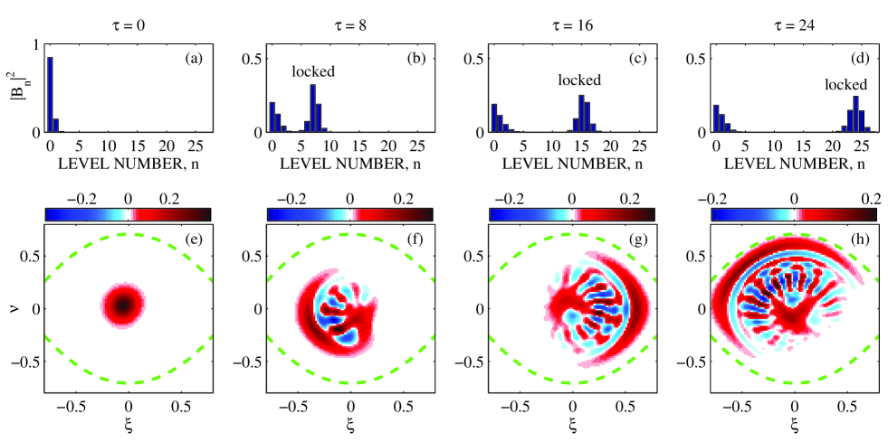
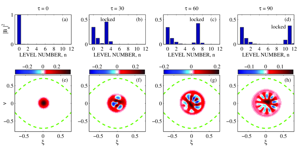
We have solved Eqs. (7) numerically, subject to ground state initial conditions at (the linear resonance corresponds to ). Each of the Figs. 1–3 corresponds to a different value of the nonlinearity parameter and show the distribution of the population of the levels in the system at four different times (subplots a-d). The subplots e-h in the Figures show the associated Wigner distributions (see Sec. V) at the same times. Figure 1 shows the case of the LC dynamics for and at , and (subplots a-d), and illustrates a clear time separation beyond the linear resonance between the successive LZ transitions. For example, we observe two groups of resonant and nonresonant levels at , separated by a valley centered at about . We find that the location of the resonant levels is determined by the slow time, i.e. , as shown above. Thus, the resonant (phase-locked) state in the system is efficiently controlled via the driving frequency and a given final state can be reached (and maintained) by terminating the frequency chirp at the desired energy level. We also see that there exists a single highly occupied level in the resonant group of levels at any given time, indicating successive LZ transitions, as expected in the LC regime.
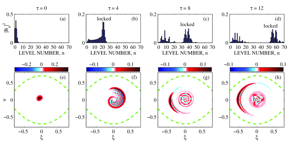
Our second numerical example is presented in Fig. 2 and illustrates the intermediate regime (as discussed above) with and , and (the subplots a-d). As in Fig. 1, a clear separation between the resonant and nonresonant groups of levels is seen in the Figure. We see that, typically, several levels are excited in the resonant group, but their number is small, so the driven dynamics can not be considered as classical. The last example (see Fig. 3) corresponds to the classical regime, , and . One observes a separation between resonant and nonresonant groups at . Note that in all our numerical examples about 50% only of the initial state is transferred to the continuing phase-locked state, leading to the question of resonant capture probability, which is discussed next.
III Resonant capture probability
III.1 Threshold for phase-locking transitions
For a given set we define the resonant capture probability,
| (9) |
where is the number of the level separating the resonant and nonresonant groups of levels at sufficiently large times. For a given value of , the probability depends on the driving parameter, For example, in the case in Fig. 1, we use and the resonant capture probability is . Similarly, in the two examples in Figs. 2 and 3, we choose to get , respectively.
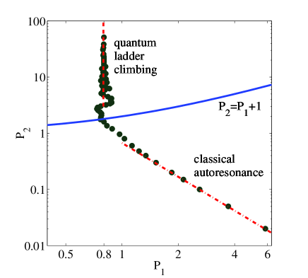
We calculate the resonant capture probability by solving Eqs. (7) numerically subject to initial conditions, (the ground state), for different values of and . For a fixed , the capture probability is a monotonically increasing, smoothed step function of . We define the threshold for efficient phase-locking transition, , as the value of for 1/2 capture probability, i.e. . The full circles in Fig. 4 show for different values of . The dashed and dashed-dotted lines are the assymptotic theoretical predictions for the quantum LC and classical AR (see below), which agree with the results of our simulations in both limits. The line is the separator between the classical and the quantum regimes of the chirped nonlinear resonance, as discussed in Sec. II. This line crosses the threshold line at . One can see in the Figure that indeed, this point separates very different dependences of on associated with the quantum and classical dynamics of the chirped system. One can also see the oscillating pattern of the threshold at , where the transition to phase-locking involves a mixture of LC and multi-level LZ steps. Next, we calculate the threshold for phase-locking transitions analytically.
III.2 Quantum-mechanical ladder climbing
In the quantum LC regime the nonlinearity parameter determines the time interval between successive resonances [see Eq. (8)]. In the case of a strong nonlinearity, at any given time only two levels are coupled, and the dynamics can be modeled by successive LZ transitions. In this case, we can calculate the probability of each transition separately, and multiply the probabilities. The two level transformation matrix (8) in the energy basis for the transition yields the transition probability via the LZ formula LZ
| (10) |
where . We define the probability for capture into resonance in this case as the probability of occupying a sufficiently high energy level after successive LZ transitions, i.e.
| (11) |
Then, solving , one finds the threshold for the LC transition,
| (12) |
where for two digits accuracy we used in the rapidly converging product (11). Thus, the capture into resonance occurs in the first few LZ transitions and one can choose (see Fig. 1 in the definition Eq. (9) for calculating the capture probability near the threshold. This prediction is valid for large , as mentioned above. The dashed line in Fig. 4 represents Eq. (12), while the numerical result for 1/2 capture probability is shown by full circles. One can see a very good agreement between the two results in the LC limit (). However, in the intermediate regime (), oscillations in are observed before convergence at the predicted LC line. These oscillations are due to the mixing of more than two neighboring levels in passage through resonance (see Fig. 2).
III.3 Classical autoresonance
As decreases, a growing number of levels are coupled simultaneously and the dynamics becomes increasingly classical. The classical AR phenomenon is now well understood Fajans . If one starts in the zero amplitude equilibrium, the autoresonant phase-locking is achieved for drives of amplitude above the critical value Fajans . When expressed in terms of , this classical threshold is translated into
| (13) |
When thermal fluctuations are included, the transition probability develops a width scaling as with temperature PRL . At the same time, the threshold for 1/2 capture probability remains the same. Thus, in Eq. (13) is the classical counterpart of the quantum-mechanical observable in Eq. (12). This classical threshold is shown in Fig. 4 by dashed-dotted line, illustrating excellent agreement with simulations (full circles) in the classical regime, . It should be emphasized that the simulation results in the Figure are solutions of the quantum-mechanical equations (7) with parameters in the classical regime, while the probabilities of capture were calculated using the proper transition level for each value of , as defined in Eq. (9). In the next Section, we discuss the width of the autoresonant transition.
IV The width of the phase-locking transition
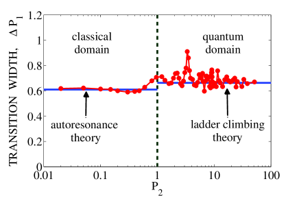
Another observable of the phase-locking transition mentioned above is the width of the transition, which we define as the inverse slope of the phase-locking probability at . This width depends on the initial conditions governed by the thermal equilibrium with the environment. Classically, the thermal width of the autoresonant transition scales as PRL
| (14) |
However, at very low temperatures, the classical thermal noise becomes negligible, but quantum fluctuations remain. Recent experiments in Josephson circuits Kater demonstrated quantum saturation of the transition width at the value obtained from Eq.(14), but with replaced by the energy of the ground level. More generally, it was suggested to calculate the width by replacing in the classical formula by an effective temperature, , in agreement with the experimental results. Using , we can translate Eq. (14) into the transition width in terms of
| (15) |
yielding
| (16) |
in the zero temperature limit. The Josephson circuit experiments Kater were performed with , i.e. well inside the classical region (see Fig. 4). Interestingly, these experiments allowed to characterize the initial quantum ”temperature” of the system by measuring the final classical autoresonant state of the chirped excitation. We will justify this approach in the next Section by analyzing the dynamics of the associated Wigner function in phase space. In contrast to Eq. (15) valid when the final state of the system is classical , the threshold width of the phase-locking transition in the LC regime () can be calculated by evaluating the slope of from Eq. (11) at , yielding
| (17) |
where we assume that the system is in the ground state initially. Figure 5 summarizes our theoretical predictions for the width of the phase-locking transition (for the same parameters as in Fig. 4) and compares them with those from numerical simulations via the Schrodinger equation (7). We see a good agreement in both the AR and LC limits, but notice significant oscillations of the width in the intermediate range of . Remarkably, while the thresholds in the classical and quantum-mechanical limits have very different scalings, the widths of the transitions are nearly the same.
V Chirped dynamics in phase space
Phase space dynamics comprises a convenient framework for comparison between classical and quantum evolution of the system. The Wigner function is one of the most useful phase space representations of the quantum mechanics, since it reduces to the classical phase space distribution in the limit of In this Section, we will study the dynamics of the Wigner function in our chirped oscillator problem in both the fixed and the rotating frames and discuss the transition to the classical limit in the problem.
V.1 Wigner dynamics in the fixed frame
The Wigner function associated with the Hamiltonian of form is governed by the quantum Liouville equation Schleich
| (18) |
where and we neglect possible decay and decoherence processes. We take a low temperature limit, neglect the nonlinearity initially, and assume that the initial state of the system is in equilibrium with the environment, i.e. Schleich ,
| (19) |
where is the effective temperature. Note that at high temperatures, while at .
In the case of interest the potential is a quartic [see Eq. (1)] and, therefore, only one term survives in the right hand side of (18), allowing to rewrite this equation in the following dimensionless form
| (20) |
where, , , , , ,
| (21) |
and . In addition, we measure time in Eq. (20) in units of and introduce the dimensionless chirp rate . With this rescaling, the initial Wigner distribution (19) becomes . We solved Eq. (20) numerically with the same parameters as in the Schrodinger simulations and show the results in Figs. 1-3 (subplots e-h) at the same times for comparison. For a better representation of the Wigner distributions for different nonlinearities, we rescaled the axis in the Figures to , and . The dashed lines in the Figures are the separatrices, enclosing all bounded classical trajectories in phase space. We started all these simulations in the ground state, i.e. , at the initial time . Figure 1 compares the dynamics in phase space to that in the energy basis in the quantum LC regime , using the parameters , , and . The pattern seen near the origin in Fig. 1 is due to the quantum interference with a finite number of states in the nonresonant region. Figure 2 shows the intermediate case for parameters , , and . Finally, Fig. 3 corresponds to the classical AR case and the parameters , , and . As well known Zurek , in the near classical case the Wigner function becomes oscillatory on increasingly fast phase space scales. However, if coarse-grained (due to a finite numerical accuracy in our case), the Wigner function becomes almost everywhere positive as one approaches the classical distribution function, despite the initial quantum-mechanical ground state used in the simulations. The evolution of the Wigner function in the last example is nearly classical with the quantum signature entering only via the effective temperature of the initial state. In the classical formula (14) for the transition width, appears due to integration over the classical Maxwell-Boltzman distribution function (see PRL ). Therefore, for the quantum-mechanical initial conditions, we should integrate over the Wigner function in a thermal state instead over the classical distribution. But these two distributions have the same functional shape, except that is replaced by in Eq. (19). Therefore, as also confirmed in experiments Kater , one can use the classical formula for the threshold of the phase-locking transition at low temperatures, when starting from quantum-mechanical initial conditions.
V.2 The dynamics in the rotating frame
Here we further expand our discussion of the classical AR limit in our system via the Wigner representation in the rotating frame. The transformation to the rotating frame is accomplished using unitary transformation (see Dykman 2006 ) where the operator and is the driving phase [see Eq. (1)]. Then, by neglecting rapidly oscillating terms, the Hamiltonian (1) is transformed to
| (22) |
where
| (23) |
The parameter in the last equation is familiar from the theory of the classical AR PRL , while is the dimensionless Plank constant, entering the commutation relation for the rescaled variables
| (24) |
Here , , where and the dimensionless time associated with the dynamics governed by Hamiltonian (23) is .
Next, we write the quantum Liouville equation in the rotating frame (see Ref. Dykman 2007 for similar developments for a constant frequency drive)
| (25) |
where . The initial Wigner distribution (19) in the new variables is
| (26) |
where . The left hand side of the Eq. (25) is identical to the Vlasov equation describing the evolution of a classical distribution of particles governed by Hamiltonian (23) without collisions and self-fields. Hence, as in the fixed frame, after coarse-graining the fast phase space oscillations of in the limit (), the dynamics in phase space can be treated classically Zurek . Therefore, both the threshold and the width of the autoresonant transition can be calculated from the classical theory as illustrated in Figs. 4 and 5, respectively, despite the quantum-mechanical initial conditions in the problem. In other words, is the measure of the classicality of the phase-locking transition in our chirped oscillator. Furthermore, in the limit of , only two parameters, and (via the initial conditions) fully characterize the AR transition. This result is in agreement with Eqs. (13) and (15) for the AR threshold and its width, where, remarkably, and enter separately.
VI Conclusions
In conclusion,
(a) We have studied the interrelation between the quantum-mechanical and classical dynamics of phase-locking transition in a Duffing oscillator driven by a chirped frequency oscillation. We studied the conditions for a continuous phase-locking in the driven system, such that the energy of the oscillator grows to stay in resonance with the varying driving frequency. The problem was defined by the temperature and three parameters, i.e. the driving amplitude the driving frequency chirp rate , and the parameter characterizing the nonlinearity of the oscillator. The nonlinearity in the problem was essential, since no persistent phase-locking in the system could be achieved for .
(b) We have exploited a more natural representation of both the quantum-mechanical and classical dynamics in the problem via just two dimensionless parameters Gilad , and instead of , and . We have shown that describes the classicality of the phase-locking transition in the system, such that, for the system arrives at its classical autoresonant (AR) state after passage through linear resonance even when starting in the quantum-mechanical ground state. In contrast, for , the transition involves the energy ladder climbing (LC) process, i.e. a continuing sequence of separated Landau-Zener transitions between neighboring energy levels. The parameters have a meaning only in the case of a finite chirp rate, which introduces a new time scale, , in the problem.
(c) The probability of transition to the phase-locked state versus has a characteristic -shape (a smoothed step function). The value of yielding 50% transition probability can be viewed as the threshold for the phase-locking transition. We have calculated this threshold and its width in both the quantum-mechanical LC and classical AR limits and compared the results to those from quantum-mechanical calculations starting in the ground state of the oscillator (see Figs. 4 and 5). We have found that, while in the LC limit the threshold is independent of , in the classical AR regime, the threshold is defined by the combination of parameters. The agreement of the theory and simulations in both limits was excellent, but characteristic oscillations of the threshold and the width were observed in the intermediate regime .
(d) We have also studied the dynamics of the phase-locking transition in phase space by using the Wigner function representation, to explain the quantum saturation of the width of the threshold for AR transitions. The analysis of the Wigner (quantum Liouville) equation in the chirped rotating frame clarifies the role of as characterizing the degree of classicality in the phase-locking transition problem.
(d) A possibility of engineering and control of a desired quantum state of the oscillator via ladder climbing process (see an example in Fig. 1) seems to be attractive in such applications as quantum computing. A generalization of this study to include possible decay, decoherence, and tunneling processes also seems to be important in future studies.
Acknowledgements.
This work was supported by the Israel Science Foundation under grant No. 451/10.References
- (1) H. Maeda, J. Nunkaew, and T.F. Gallagher, Phys. Rev. A 75, 053417 (2007).
- (2) S. Chelkowski and A. Bandrauk, J. Chem. Phys. 99, 4279 (1993).
- (3) A. Barak, Y. Lamhot, L. Friedland, and M. Segev, Phys. Rev. Lett. 103, 123901 (2009).
- (4) O. Naaman, J. Aumentado, L. Friedland, J.S. Wurtele, and I. Siddiqi, Phys. Rev. Lett. 101, 117005 (2008).
- (5) O. Ben-David, M. Assaf, J. Fineberg, and B. Meerson, Phys. Rev. Lett. 96, 154503 (2006).
- (6) J.R. Danielson, T.R. Weber, and C.M. Surko, Phys. Plasmas 13, 123502 (2006).
- (7) L. Friedland, Phys. Rev. Lett. 69, 1749 (1992).
- (8) G. Manfredi and P.A. Hervieux, App. Phys. Lett. 91, 061108 (2007).
- (9) G.B. Andresen et al. (ALPHA Collaboration), Nature (London) 468, 673 (2010).
- (10) G.B. Andresen et al. (ALPHA Collaboration), Phys. Rev. Lett 106, 025002 (2011).
- (11) K.W. Murch, R. Vijay, I. Barth, O. Naaman, J. Aumentado, L. Friedland, and I. Siddiqi, Nature Physics 7, 105 (2011).
- (12) G. Marcus, L. Friedland, and A. Zigler, Phys. Rev. A 69, 013407 (2004).
- (13) G. Marcus, A. Zigler, and L. Friedland, Europhys. Lett. 74, 43 (2006).
- (14) J. Fajans and L. Friedland, Am. J. Phys. 69, 1096 (2001).
- (15) I. Barth, L. Friedland, E. Sarid, and A.G. Shagalov, Phys. Rev. Lett. 103, 155001 (2009).
- (16) L.D. Landau, Phys. Z. Sowjetunion 2, 46 (1932); C. Zener, Proc. R. Soc. London A137, 696 (1932).
- (17) M.E. Goggin and P.W. Milonni, Phys. Rev. A 37, 796 (1988).
- (18) L. Landau and E.M. Lifshitz, Quantum Mechanics (Non-Relativistic Theory), 3rd ed. (Butterworth Heinemann, Oxford, 1977) p. 136.
- (19) N.V. Vitanov and B.M. Garraway, Phys. Rev. A 53, 4288 (1996).
- (20) W.P. Schleich, Quantum Optics in Phase Space, (Wiley-VCH Verlag, Berlin, 2001), Chap. 3.3, p.75.
- (21) see, for example, W.H. Zurek, Rev. Mod. Phys. 75, 715 (2003).
- (22) M. Marthaler and M.I. Dykman, Phys. Rev. A 73, 042108 (2006).
- (23) M.I. Dykman, Phys. Rev. E 75, 011101 (2007).