Practical and Efficient Circle Graph Recognition

Abstract

Circle graphs are the intersection graphs of chords in a circle. This paper presents the first sub-quadratic recognition algorithm for the class of circle graphs. Our algorithm is $O(n+m)$ times the inverse Ackermann function, $\alpha(n+m)$, whose value is smaller than 4 for any practical graph. The algorithm is based on a new incremental Lexicographic Breadth-First Search characterization of circle graphs, and a new efficient data-structure for circle graphs, both developed in the paper. The algorithm is an extension of a Split Decomposition algorithm with the same running time developed by the authors in a companion paper.

1 Introduction

A chord diagram can be defined as a circle inscribed by a set of chords. A graph is a circle graph if it is the intersection graph of a chord diagram: the vertices correspond to the chords, and two vertices are adjacent if and only if their chords intersect. Combinatorially, chord diagrams are defined by double occurence circular words. Circle graphs were first introduced in the early 1970s, under the name alternance graphs, as a means of sorting permutations using stacks [10]. The polynomial time recognition of circle graphs was posed as an open problem by Golumbic in the first edition of his book [16]. The question received considerable attention afterwards and was eventually settled independently by Naji [19], Bouchet [1], and Gabor et al. [11].

Bouchet’s $O(n^{5})$ algorithm is based on a characterization of circle graphs in terms of local complementation, a concept originated in his work on isotropic systems [2], of which the recently introduced rank-width and vertex-minor theories are extensions [20, 12]. It is conjectured that circle graphs are related to rank-width and vertex-minors as planar graphs are related to tree-width and graph-minors: just as large tree-width implies the existence of a large grid as a graph-minor, it is conjectured that large rank-width implies the existence of a large circle graph vertex-minor [21]. The conjecture has already been verified for line-graphs [21].

Both Naji’s $O(n^{7})$ algorithm and Gabor et al.’s $O(n^{3})$ algorithm are based on split decomposition, introduced by Cunningham [7]. A split is a bipartition $(A,B)$ (with $|A|,|B|>1$) of a graph’s vertices, where there are subsets (called the frontiers) $A^{\prime}\subseteq A$ and $B^{\prime}\subseteq B$ such that no edges exist between $A$ and $B$ other than those between $A^{\prime}$ and $B^{\prime}$, and every possible edge exists between $A^{\prime}$ and $B^{\prime}$. Intuitively, split decomposition finds a split and recursively decomposes its parts. A graph is called prime if it does not contain a split. It is known that a graph is a circle graph if and only if its prime split decomposition components are circle graphs [11]. This property is used by Bouchet, Naji, and Gabor et al. to reduce the recognition of circle graphs to the recognition of prime circle graphs. The latter problem is made somewhat easier by the fact that prime circle graphs have unique chord diagrams (up to reflection) [1] (see also [6]).

The algorithm of Gabor et al. was improved by Spinrad in 1994 to run in time $O(n^{2})$ [23]. A key component is an $O(n^{2})$ prime testing procedure he developed with Ma [18]. A linear time prime testing procedure now exists in the form of Dahlhaus’ split decomposition algorithm [8]; however, a faster circle graph recognition algorithm has not followed. In fact, the complexity bottleneck in Spinrad’s algorithm is not computing the split decomposition, but rather his procedure to construct the unique chord diagram for prime circle graphs.

This paper presents the first sub-quadratic circle graph recognition algorithm. Our algorithm runs in time $O(n+m)\alpha(n+m)$, where $\alpha$ is the inverse Ackermann function [3, 24]. We point out that this function is so slowly growing that it is bounded by $4$ for all practical purposes.

We overcome Spinrad’s bottleneck in two ways: we use the recent reformulation of split decomposition in terms of graph-labelled trees (GLTs) [13, 14], and we derive a new characterization of circle graphs in terms of Lexicographic Breadth-First Search (LBFS) [22]. The key technical concept we deal with is that of consecutiveness in a chord diagram (Section 3), a property that can be efficiently preserved under a certain GLT transformation (Section 3.1). On one hand, this concept provides a new property for chord diagrams of the components in the split decomposition of a circle graph (Section 3.2). On the other hand, it provides a new property for prime circle graphs with respect to an LBFS ordering (Section 3.3). Finally, these results allow us to characterize how a prime circle graph can be built incrementally, according to an LBFS ordering (Section 3.4).

This treatment of prime circle graphs can be integrated with the incremental split decomposition algorithm from the companion paper [15], whose running time is $O(n+m)\alpha(n+m)$. That algorithm operates in the GLT setting, computing the split decomposition incrementally, only it adds vertices according to an LBFS ordering (Section 4). Throughout that process, our proposed circle graph recognition algorithm maintains chord diagrams for all prime components in the split decomposition so long as possible. We do so by applying the new results mentioned above for prime circle graphs in an incremental LBFS setting. A new data-structure for chord diagrams is developed in the paper so that these results can be efficiently implemented (Section 5). In particular, our new data-structure is what enables the efficiency of the GLT transformations that preserve consecutiveness. Our results represent substantial progress on a long-standing open problem.

2 Preliminaries

2.1 Basic Definitions and Terminology

All graphs in this document are simple, undirected, and connected. The set of vertices in the graph $G$ is denoted $V(G)$ (or $V$ when the context is clear). The subgraph of $G$ induced on the set of vertices $S$ is signified by $G[S]$. We let $N_{G}(x)$, or simply $N(x)$, denote the set of neighbours of $x$, and if $S$ is a set of vertices, then $N(S)=(\cup_{x\in S}N(x))\setminus S$. A vertex is universal to a set of vertices $S$ if it is adjacent to every vertex in $S$. A vertex is universal in a graph if it is adjacent to every other vertex in the graph. A clique is a graph in which every pair of vertices is adjacent. We require in this paper that cliques have at least three vertices. A star is a graph with at least three vertices in which one vertex, called its centre, is universal, and no other edges exist. Cliques and stars are called degenerate with respect to split decomposition as every non-trivial bipartition of their vertices forms a split. Given two connected graphs $G$ and $G^{\prime}$, each having at least two vertices, and given two vertices $q\in V(G)$ and $q^{\prime}\in V(G^{\prime})$, the join between $G$ and $G^{\prime}$ with respect to $q$ and $q^{\prime}$, denoted by $(G,q)\otimes(G^{\prime},q^{\prime})$, is the graph formed from $G$ and $G^{\prime}$ as follows: all possible edges are added between $N_{G}(q)$ and $N_{G^{\prime}}(q^{\prime})$, and then $q$ and $q^{\prime}$ are deleted. In this case, observe that $(V(G)\setminus\{q\},V(G^{\prime})\setminus\{q^{\prime}\})$ is a split of the graph $(G,q)\otimes(G^{\prime},q^{\prime})$.

The graph $G+(x,N(x))$ is formed by adding the vertex $x$ to the graph $G$ adjacent to the subset $N(x)$ of vertices, its neighbourhood; when $N(x)$ is clear from the context we simply write $G+x$. The graph $G-x$ is formed from $G$ by removing $x$ and all its incident edges.

To avoid confusion with graphs, the edges of a tree are called tree-edges. If $T$ is a tree, then $|T|$ represents the number of its vertices. The non-leaf vertices of a tree are called its nodes. The tree-edges not incident to leaves are internal tree-edges.

2.2 The Split-Tree of a Graph

The split decomposition and the related split-tree play a central role in the circle graph recognition problem. This subsection essentially recalls definitions from [13, 14] and from [15]. Here, we will give only the material required in the present paper. More involved definitions and details are given in [15]. Let us mention that the graph-labelled tree sructure defined below can be easily related to other representations used for the split decomposition, e.g. [5, 7].

Definition 2.1 ([13, 14]).

A graph-labelled tree (GLT) is a pair $(T,\mathcal{F})$, where $T$ is a tree and $\mathcal{F}$ a set of graphs, such that each node $u$ of $T$ is labelled by the graph $G(u)\in\mathcal{F}$, and there exists a bijection $\rho_{u}$ between the edges of $T$ incident to $u$ and the vertices of $G(u)$. (See Figure 1.)

Figure 1: On the left: a graph-labelled tree $(T,\mathcal{F})$; on the right: its accessibility graph ${Gr}(T,\mathcal{F})$. For the pictured marker vertex $q$, we have $L(q)=\{1,2,3,4,5,6,7\}$. The leaves accessible from $q$ are $\{1,3,4,7,14,15\}$, and we have $A(q)=\{1,3,4,7\}$.

When we refer to a node $u$ in a GLT $(T,\mathcal{F})$, we usually mean the node itself, although we may sometimes use the notation $u$ as a shorthand for its label $G(u)\in\mathcal{F}$, the meaning being clear from context; for instance, notation will be simplified by saying $V(u)=V(G(u))$. The vertices in $V(u)$ are called marker vertices, and the edges between them in $G(u)$ are called label-edges. For a label-edge $e=uv$ we may say that $u$ and $v$ are the (marker) vertices of $e$. For the internal tree-edge $e=uv$, we say the marker vertices $\rho_{u}(e)$ and $\rho_{v}(e)$ are the extremities of $e$. For convenience, we may say that a tree-edge and its extremities are incident. Furthermore, $\rho_{v}(e)$ is the opposite of $\rho_{u}(e)$ (and vice versa). A leaf is also considered an extremity of its incident tree-edge, and its opposite is the other extremity of that tree-edge (marker vertex or leaf). Sometimes a marker vertex will simply be said to be opposite a leaf or another marker vertex, the meaning in this case being that implied above. If $q$ is a marker vertex such that $\rho_{u}(e)=q$, then we let $L(q)$ denote the set of leaves of the tree not containing $u$ in the forest $T-e$; see Figure 1 where $L(q)=\{1,2,3,4,5,6,7\}$. Extending this notion to leaves, the set $L(\ell)$ for the leaf $\ell$ is equal to all leaves in $T$ different from $\ell$. The central notion for GLTs with respect to split decomposition is that of accessibility:

Definition 2.2 ([13, 14]).

Let $(T,\mathcal{F})$ be a GLT. Two marker vertices $q$ and $q^{\prime}$ are accessible from one another if there is a sequence $\Pi$ of marker vertices $q,\ldots,q^{\prime}$ such that:

1. every two consecutive elements of $\Pi$ are either the vertices of a label-edge or the extremities of a tree-edge;

2. the edges thus defined alternate between tree-edges and label-edges.

Two leaves are accessible from one another if their opposite marker vertices are accessible; similarly for a leaf and marker vertex being accessible from one another; see Figure 1 where the leaves accessible from $q$ include both 3 and 15 but neither 2 nor 11. By convention, a leaf or marker vertex is accessible from itself.

Note that, obviously, if two leaves or marker vertices are accessible from one another, then the sequence $\Pi$ with the required properties is unique, and the set of tree-edges in $\Pi$ forms a path in the tree $T$. If $q$ is a marker vertex, then we let $A(q)$ denote the set of leaves in $L(q)$ accessible from $q$; see Figure 1. The set $A(\ell)$ is similarly defined for a leaf $\ell$.

Definition 2.3 ([13, 14]).

Let $(T,\mathcal{F})$ be a GLT. Then its accessibility graph, denoted ${Gr}(T,\mathcal{F})$, is the graph whose vertices are the leaves of $T$, with an edge between two distinct vertices if and only if the corresponding leaves are accessible from one another. Conversely, we may say that $(T,\mathcal{F})$ is a GLT of ${Gr}(T,\mathcal{F})$.

Accessibility allows us to view GLTs as encoding graphs; an example appears in Figure 1. The following remarks directly follow from Definition 2.3:

Remark 2.4.

A graph $G$ is connected if and only if every label in a GLT of $G$ is connected.

Remark 2.5.

Let $(T,\mathcal{F})$ be a GLT, with ${Gr}(T,\mathcal{F})$ connected. For every marker vertex $q$ in $(T,\mathcal{F})$, $A(q)$ is non-empty.

Remark 2.6.

Let $e$ be an internal tree-edge of a GLT $(T,\mathcal{F})$, with ${Gr}(T,\mathcal{F})$ connected, and let $p$ and $q$ be the two extremities of $e$. Then the bipartition $(L(p),L(q))$ is a split of ${Gr}(T,\mathcal{F})$. Moreover $A(q)$ and $A(p)$ are the frontiers of that split.

Remark 2.7.

Let $(T,\mathcal{F})$ be a GLT, with ${Gr}(T,\mathcal{F})$ connected. For every graph label $G(u)$ in $\mathcal{F}$, there exists a subset $L$ of leaves of $T$ such that $G(u)$ is isomorphic to the subgraph of ${Gr}(T,\mathcal{F})$ induced by $L$. Note that $L$ can be built by choosing, for every vertex $q$ of $G(u)$, an element of $A(q)$.

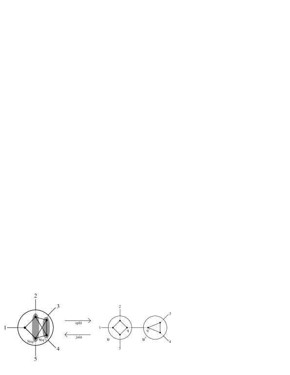
Figure 2: Example of the node-join and node-split.

Let $e=uu^{\prime}$ be an internal tree-edge of a GLT $(T,\mathcal{F})$, and let $q\in V(u)$ and $q^{\prime}\in V(u^{\prime})$ be the extremities of $e$. The node-join of $u$ and $u^{\prime}$ is the following operation: contract the tree-edge $e$, yielding a new node $v$ labelled by the join between $G(u)$ and $G(u^{\prime})$ with respect to $q$ and $q^{\prime}$. Every other tree-edge and their pairs of extremities are preserved. The node-split is the inverse of the node-join. Both operations are illustrated in Figure 2. A key property to observe is that the node-join operation and the node-split operation preserve the accessibility graph of the GLT.

To end this subsection, we recall the main result of split decomposition theory [7], which we restate below in terms of GLTs, as in [13, 14]:

Theorem 2.8 ([7, 13, 14]).

For any connected graph $G$, there exists a unique graph-labelled tree $(T,\mathcal{F})$ whose labels are either prime or degenerate, having a minimal number of nodes, and such that ${Gr}(T,\mathcal{F})=G$.

Definition 2.9.

The unique graph-labelled tree guaranteed by Theorem 2.8 is called the split-tree for $G$, and is denoted $ST(G)$.

For example, the GLT in Figure 1 is the split-tree for the accessibility graph pictured there. The split-tree of a graph $G$ could be thought as a representation of the set of splits: it is known that every split either corresponds to a tree-edge of the split-tree or to the tree-edge resulting from a node-split of some degenerate-node (for more details, the reader should refer to the companion paper [15]).

2.3 Lexicographic Breadth-First Search

Lexicographic Breadth-First Search (LBFS) was developed by Rose, Tarjan, and Lueker for the recognition of chordal graphs [22], and has since become a standard tool in algorithmic graph theory [4]. It appears here as Algorithm 1.

Input: A graph $G$ with $n$ vertices.

Output: An ordering $\sigma$ of $V(G)$ defined by a mapping $\sigma:V(G)\rightarrow\{1,\ldots,n\}$.

foreach $x\in V(G)$ do label($x$) $\leftarrow\epsilon$ (the empty-string) ;

;

for $i=1$ to $n$ do

       pick an unnumbered vertex $x$ with lexicographically largest label;

       $\sigma(x)\leftarrow i$ ;

       // assign $x$ the number $i$

       foreach unnumbered vertex $y\in N(x)$ do append $n-i+1$ to label($y$);

      ;

      

end for

Algorithm 1 Lexicographic Breadth-First Search

By an LBFS ordering of the graph $G$ (or its set of vertices $V(G)$), we mean any ordering $\sigma$ produced by Algorithm 1 when the input is $G$. We write $x<_{\sigma}y$ if $\sigma(x)<\sigma(y)$. Notice that the first vertex in any LBFS ordering is arbitrary. This is because all vertices start out with the empty string label. More generally, the vertex with the lexicographically largest label may not be unique. As another example, if $x$ is numbered first, meaning it is the first vertex in the LBFS ordering, then every vertex in $N(x)$ will share the lexicographically largest label at the time the second vertex is numbered. In other words, any vertex in $N(x)$ can follow $x$ in an LBFS ordering. Interestingly, LBFS orderings can be characterized as follows:

Lemma 2.10 ([9][16]).

An ordering $\sigma$ of a graph $G$ is an LBFS ordering if and only if for any triple of vertices $a<_{\sigma}b<_{\sigma}c$ with $ac\in E(G)$, $ab\notin E(G)$, there is a vertex $d<_{\sigma}a$ such that $db\in E(G)$, $dc\notin E(G)$.

For a subset $S$ of $V(G)$, we denote $\sigma[S]$ as the restriction of $\sigma$ to $S$: that is, for $x,y\in S$, $x<_{\sigma[S]}y$ if and only if $x<_{\sigma}y$. A prefix of $\sigma$ is a subset $S$ such that $x<_{\sigma}y$ and $y\in S$ implies that $x\in S$.

The following remarks are obvious and well-known observations:

Remark 2.11.

If $\sigma$ is an LBFS ordering of a graph $G$, and $x$ is a universal vertex in $G$, then $\sigma[V(G)-\{x\}]$ is an LBFS ordering of $G-x$.

Remark 2.12.

Let $S$ be a prefix of any LBFS ordering $\sigma$ of a graph $G$. Then $\sigma[S]$ is an LBFS ordering of $G[S]$.

Our circle graph recognition algorithm is based on special properties of good vertices and on the hereditary property of LBFS orderings with respect to the label graphs of a GLT (and thus of the split-tree).

Definition 2.13.

A vertex $x\in V(G)$ is good for the graph $G$ if there is an LBFS ordering of $G$ in which $x$ appears last.

Definition 2.14 (Definition 3.5 in [15]).

Let $u$ be a node of a GLT $(T,\mathcal{F})$ and let $\sigma$ be an LBFS ordering of $G=Gr(T,\mathcal{F})$. For any marker vertex $p$, let $x_{p}$ be the earliest vertex of $A(p)$ in $\sigma$. Define $\sigma_{u}$ to be the ordering of $G(u)$ such that for $q,r\in V(u)$, $q<_{\sigma_{u}}r$ if $x_{q}<_{\sigma}x_{r}$.

Lemma 2.15 (Lemma 3.6 in [15]).

Let $\sigma$ be an LBFS ordering of graph $G=Gr(T,\mathcal{F})$, and let $u$ be a node in $(T,\mathcal{F})$. Then $\sigma_{u}$ is an LBFS ordering of $G(u)$.

2.4 Circle Graphs

We will work with circle graphs using a variant of the double occurrence words mentioned in the introduction. A word over an alphabet $\Sigma$ is a sequence of letters of $\Sigma$. If $S$ is a word over $\Sigma$, then $S^{r}$ denotes the reversed sequence of letters. The concatenation of two words $A$ and $B$ is denoted $AB$. A circular word $C$ over an alphabet $\Sigma$ is a circular sequence of letters of $\Sigma$; they can be represented by a word $S$ by considering that the first letter of $S$ follows its last letter. That is: if $S$ is the concatenation $AB$ of the words $A$ and $B$, then $BA$ represents the same circular word $C$ as $S=AB$, and we denote this by $C\sim AB\sim BA$. A factor of a word (respectively of a circular word), over $\Sigma$ is a sequence of consecutive letters in this word (respectively in a word representing this circular word). Formally, we may sometimes make the abuse to consider a factor of a given (circular) word as a set of letters, and conversely, as soon as this set of letters forms a factor in this (circular) word. If the sequence $S$ of elements of $\Sigma$ defines a circular word $C$, then the reversed sequence $S^{r}$ defines the reflection of $C$, denoted $C^{r}$.

We define formally the chord diagrams mentioned in the introduction using circular words. For a set $V$, called a set of chords, a chord diagram on $V$ is a circular word on the alphabet ${\mathcal{V}}=\bigcup_{v\in V}\{v_{1},v_{2}\}$ where every letter appears exactly once. The elements of ${\mathcal{V}}$ are called endpoints, and, for every chord $v\in V$, the letters $v_{1}$ and $v_{2}$ of ${\mathcal{V}}$ are called the endpoints of $v$. Geometrically, a chord diagram can be represented as a circle inscribed by a set of chords (see figure 3). Now, if $C$ is a chord diagram on $V$, then the simple chord diagram induced by $C$ is the circular word $\bar{C}$ on $V$ obtained by replacing the endpoints appearing in $C$ by the corresponding chords of $V$ (or equivalently, removing the subscripts from the endpoints). If $a$ and $b$ are two endpoints of the chord diagram $C\sim AaBbA^{\prime}$, with $A,B,A^{\prime}$ words on ${\mathcal{V}}$, then we define the factor $C(a,b)=B$. Based on this, it follows that $C(b,a)=A^{\prime}A$, and similarly $C^{r}(a,b)=A^{r}A^{\prime r}$ and $C^{r}(b,a)=B^{r}$.

The chord diagram $C$ encodes the graph $G=(V,E)$ as follows: the chords of $C$ correspond to the vertices $V$, two of which are adjacent if and only if their corresponding chords intersect. Using the notation from above, vertices $x$ and $y$ are adjacent if and only if the factor $C(x_{1},x_{2})$ contains either $y_{1}$ or $y_{2}$ but not both. The circle graphs are the graphs that can be encoded by chord diagrams in this way. We say that $C$ is a chord diagram for $G$, or that $C$ encodes $G$. The above definitions are naturally extended to simple chord diagrams. Notice that if $C$ is a chord diagram for $G$, then $C^{r}$ is a chord diagram for $G$ as well. An example appears in Figure 3.

Figure 3: A chord diagram $C$ drawn on a circle (on the left) and the corresponding circle graph $G$ (on the right). By convention we read the sequences clockwise from figures. We have $C(a_{2},f_{2})=h_{1}e_{1}b_{2}a_{1}d_{1}$ and $C(f_{2},a_{2})=e_{2}g_{1}f_{1}h_{2}g_{2}c_{1}d_{2}b_{1}c_{2}$.

If $L\subseteq V(G)$, then $C[L]$ is the chord diagram formed by removing from $C$ all chords corresponding to vertices not in $L$.

Remark 2.16.

If $C$ is a chord diagram for $G$, and $L\subseteq V(G)$, then $C[L]$ is a chord diagram for $G[L]$.

Simple chord diagrams are in general not uniquely determined by the graph they encode, as demonstrated by the example of cliques and stars (depicted in Figure 4). A chord diagram $C$ of a clique $G$ is of the form $C\sim AA$, where $A$ is any permutation of its vertices. If $G$ is a star with centre vertex $c$, a chord diagram $C$ is of the form $C\sim cAcA^{r}$, where $A$ is any permutation of the non-centre vertices of the star. In both cases, one can transpose any two chords (distinct from the centre, in the case of a star). On the contrary, it is known that if a circle graph is prime (i.e. has no split) then it has a unique simple chord diagram (up to reflection), and that the converse is true provided the graph has more than four vertices [1] (see also [6]).

Figure 4: A simple chord diagram for a clique; a simple chord diagram for a star.

The concept of join between two graphs $G$ and $G^{\prime}$ with respect to two vertices $q\in V(G)$ and $q^{\prime}\in V(G^{\prime})$ was defined in Section 2.1. A similar join operation directly applies to chord diagrams. It will be thoroughly used in our incremental split-tree construction of circle graphs.

Definition 2.17.

Let $C$ and $C^{\prime}$ be chord diagrams on $V$ and $V^{\prime}$, respectively, and let $q$ belong to $V$ and $q^{\prime}$ belong to $V^{\prime}$. We define a circle-join operation between $C$ and $C^{\prime}$ with respect to $q$ and $q^{\prime}$ as follows

$$(C,q)\odot(C^{\prime},q^{\prime})\ \sim\ C(q_{1},q_{2})C^{\prime}(q^{\prime}_{1},q^{\prime}_{2})C(q_{2},q_{1})C^{\prime}(q^{\prime}_{2},q^{\prime}_{1})$$

Observe that the circle-join is not commutative. We may use the notation $(C,q)\ \hat{\odot}\ (C^{\prime},q^{\prime})$ instead of $(C^{\prime},q^{\prime})\ \odot\ (C,q)$. By construction, the resulting sequences of letters define chord diagrams on the set of chords $(V\setminus\{q\})\cup(V^{\prime}\setminus\{q^{\prime}\})$. An illustration of this construction and of the obvious remark below is given in Figure 5.

Figure 5: A circle-join $(C,q)\odot(C^{\prime},q^{\prime})$, and the corresponding node-join between graphs $G$ and $G^{\prime}$ encoded by $C$ and $C^{\prime}$ respectively (Remark 2.18).

Remark 2.18.

Let $C$ and $C^{\prime}$ be chord diagrams of $G$ and $G^{\prime}$, respectively, and let $q$ belong to $V(G)$ and $q$ belong to $V(G^{\prime})$. The chord diagrams $(C,q)\odot(C^{\prime},q^{\prime})$ and $(C,q)\ \hat{\odot}\ (C^{\prime},q^{\prime})$ encode the graph $H=(G,q)\otimes(G^{\prime},q^{\prime})$.

Assume that $G^{\prime}$ and $C^{\prime}$ are as in Remark 2.18. Let us also remark that, as $C^{\prime r}$ is a chord diagram of $G^{\prime}$, both $(C,q)\odot(C^{\prime r},q^{\prime})$ and $(C,q)\ \hat{\odot}\ (C^{\prime r},q^{\prime})$ are also chord diagrams of the same graph $H$. Finally, Remark 2.18 also allows us to obtain the following well-known result, restated in terms of graph-labelled trees:

Corollary 2.19.

Let $(T,\mathcal{F})$ be a GLT. The accessiblity graph ${Gr}(T,\mathcal{F})$ is a circle graph if and only if for every node $u$ in $T$, the label $G(u)$ is a circle graph.

Proof.

Notice that by recursively performing node-joins, any GLT can be reduced to a single node labelled by its accessibility graph. Thus, by Remark 2.18, if every label in the GLT is a circle graph, then so is its accessibility graph. For the converse, notice that every label in a GLT is isomorphic to an induced subgraph of its accessibility graph (Remark 2.7). Since every induced subgraph of a circle graph is also a circle graph (Remark 2.16), if $G$ is a circle graph, so is every label in a GLT having $G$ as its accessibility graph. ∎

3 Consecutiveness and LBFS Incremental Characterization

The key technical concept for this paper is given by the definition below of consecutiveness. Subsections 3.1, 3.2 and 3.3 that follow are independent from each other and provide general properties of circle graphs with respect to consecutiveness. Their results will be merged in Subsection 3.4 with the incremental construction of the split-tree from [15] to get the main theorem of this section.

Definition 3.1.

Let $C$ be a chord diagram on a set $V$ of chords. If a set of endpoints $S_{e}\subseteq{\mathcal{V}}$ is a factor of $C$ (i.e. appears consecutively), then the first and last endpoint in this factor are called bookends for $S_{e}$.

Definition 3.2.

A set of chords $S\subseteq V$ is consecutive in $C$ if $C$ contains a set of endpoints $S_{e}\subseteq{\mathcal{V}}$ as a factor such that $|S_{e}\cap\{x_{1},x_{2}\}|=1$ for all $x\in S$, and $S_{e}\cap\{x_{1},x_{2}\}=\emptyset$ for all $x\notin S$. In this case, $S_{e}$ certifies the consecutiveness of $S$, and a vertex $x\in S$ is a bookend for $S$ if one of its endpoints is a bookend for $S_{e}$. The definition naturally extends to a simple chord diagram $\bar{C}$ by considering any chord diagram $C$ whose underlying simple chord diagram is $\bar{C}$.

Observe that if $S$ is a consecutive set of at least two chords, then two distinct chords of $S$ are bookends. On the chord diagram $C$ depicted in Figure 5, the consecutiveness of the subset of chords $S=\{b,c,d\}$ is certified by $S_{e}=\{c_{1},d_{2},b_{1}\}$; the bookends of $S_{e}$ are $c_{1}$ and $b_{1}$, meaning $b$ and $c$ are bookends for $S$.

3.1 Circle-Join Property

Lemma 3.3 below will be crucial (in Section 3.4) for maintaining chord diagrams during the vertex insertions constructing the split-tree in the companion paper [15]. It is illustrated in Figure 6 below.

Lemma 3.3.

Let $C$ and $C^{\prime}$ be chord diagrams on the sets of chords $V$ and $V^{\prime}$ respectively. Let $S\subset V$ and $S^{\prime}\subset V^{\prime}$ be sets of chords such that $1<\mid S\mid<\mid V\mid$ and $1<\mid S^{\prime}\mid<\mid V^{\prime}\mid$. Assume that $S$ and $S^{\prime}$ are consecutive in their respective chord diagrams. If $q$ is a bookend of $S$, and $q^{\prime}$ is a bookend of $S^{\prime}$, then the set of chords $(S\setminus\{q\})\cup(S^{\prime}\setminus\{q^{\prime}\})$ is consecutive in (at least) one of the following chord diagrams, with bookends being those of $S$ and $S^{\prime}$ other than $q$ and $q^{\prime}$:

$$(C,q)\odot(C^{\prime},q^{\prime}),~{}~{}~{}~{}~{}~{}(C,q)\ \hat{\odot}\ (C^{\prime},q^{\prime}),~{}~{}~{}~{}~{}~{}(C,q)\odot(C^{\prime r},q^{\prime}),~{}~{}~{}~{}~{}~{}(C,q)\ \hat{\odot}\ (C^{\prime r},q^{\prime}).$$

Proof.

Assume that the consecutiveness of $S$ in $C$ is certified by the set $S_{e}$ of endpoints and, without loss of generality, let $q_{1}$ be the endpoint of $q$ in $S_{e}$. Let $r_{1}$ denote the other bookend of $S_{e}$ with chord $r$ distinct from $q$. Similarly assume that the consecutiveness of $S^{\prime}$ in $C^{\prime}$ is certified by the set $S^{\prime}_{e}$ of endpoints, and without loss of generality let $q^{\prime}_{1}$ be the endpoint of $q^{\prime}$ in $S^{\prime}_{e}$. Let $r^{\prime}_{1}$ denote the other bookend of $S^{\prime}_{e}$ with chord $r^{\prime}$ distinct from $q^{\prime}$. Observe that either $S_{e}$ is a factor of (but not equal to) $q_{1}C(q_{1},q_{2})$ or of $C(q_{2},q_{1})q_{1}$. Assume the former. Observe also that either $S^{\prime}_{e}$ is a factor of (but not equal to) $q^{\prime}_{1}C^{\prime}(q^{\prime}_{1},q^{\prime}_{2})$ or of $C^{\prime}(q^{\prime}_{2},q^{\prime}_{1})q^{\prime}_{1}$. Assume the former. We complete the proof under these two assumptions, the other cases are similar.

Let $a$ and $b$ be the first and last endpoints of $C(q_{1},q_{2})$. Observe that $a\in S_{e}$ and $b\notin S_{e}$ and thus $b$ is not an endpoint of $r$. Let $a^{\prime}$ and $b^{\prime}$ be the first and last endpoints of $C^{\prime}(q^{\prime}_{1},q^{\prime}_{2})$. Observe that $a^{\prime}\in S^{\prime}_{e}$ and $b^{\prime}\notin S^{\prime}_{e}$ and thus $b^{\prime}$ is not an endpoint of $r^{\prime}$. By construction, $a$ and $a^{\prime}$ appear consecutively on $(C,q)~{}\odot~{}(C^{\prime r},q^{\prime})$. Then $(S\setminus\{q\})\cup(S^{\prime}\setminus\{q^{\prime}\})$ is consecutive and has bookends $r_{1}$ and $r^{\prime}_{1}$. ∎

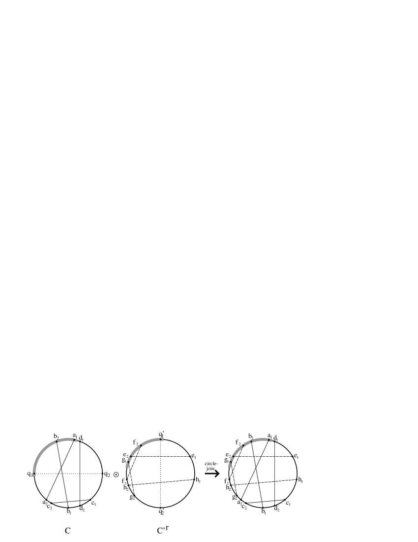
Figure 6: A consecutivity preserving circle-join requiring a reflection (Lemma 3.3 with $S=\{q,a,b\}$ and $S^{\prime}=\{q^{\prime},f,e,g\}$). Here $C^{\prime r}$ is the reflection of $C^{\prime}$ from Figure 5. The resulting chord diagram is $(C,q)\odot(C^{\prime r},q^{\prime})$, where $\{a,b,f,e,g\}$ is consecutive with inherited bookends $a$ and $g$.

3.2 Split-Tree Property

This subsection shows how a consecutive set of chords/vertices in a chord diagram $C$ of a circle graph $G$ induces a consecutive set of chords/vertices of the chord diagram of the circle graph $G(u)$ for any node $u$ of the split-tree $ST(G)$. The proof relies on the following result, which can be found in an equivalent form as proposition 9 in [6].

Proposition 3.4 (Proposition 9 in [6]).

Let $C$ be a chord diagram for the circle graph $G$. Let $q$ and $r$ be the extremities of a tree-edge in $ST(G)$. Then $C$ can be partitioned into four factors $C\sim A_{1}B_{1}A_{2}B_{2}$ such that $A_{1}\cup A_{2}=\bigcup_{x\in L(q)}\{x_{1},x_{2}\}$ and $B_{1}\cup B_{2}=\bigcup_{y\in L(r)}\{y_{1},y_{2}\}$.

Together with Remark 2.6, the above proposition yields the following:

Corollary 3.5.

Let $q$ and $r$ be the extremities of a tree-edge in $ST(G)$. Let $C\sim A_{1}B_{1}A_{2}B_{2}$ be a chord diagram for the circle graph $G$ such that $A_{1}\cup A_{2}=\bigcup_{x\in L(q)}\{x_{1},x_{2}\}$ and $B_{1}\cup B_{2}=\bigcup_{y\in L(r)}\{y_{1},y_{2}\}$. Consider an arbitrary leaf $l$ in $ST(G)$. Then $l$ is in $A(q)$ if and only if it has one endpoint in $A_{1}$ and the other in $A_{2}$.

Proof.

By Remark 2.6, $A(q)$ and $A(r)$ are the frontiers of the split $(L(q),L(r))$ in $G$. In other words, every leaf of $A(r)$ is adjacent in $G$ to every leaf of $A(q)$. Equivalently, these pairs of leaves correspond to intersecting pairs of chords $l,l^{\prime}$ such that $l\in A_{1}\cup A_{2}$ and $l^{\prime}\in B_{1}\cup B_{2}$. Observe that this holds if and only if $l$ (respectively $l^{\prime}$) has one endpoint in $A_{1}$ (respectively $B_{1}$) and the other in $A_{2}$ (respectively $B_{2}$). ∎

If $u$ is a node of $ST(G)$, then applying proposition 3.4 on every tree-edge incident to $u$, we obtain:

Corollary 3.6.

Let $C$ be a chord diagram encoding the circle graph $G$. If $u$ is a node of degree $k$ in $ST(G)$, then $C$’s endpoints can be partitioned into $2k$ factors $C\sim A_{1}A_{2}\dots A_{2k-1}A_{2k}$ such that for every $q$ in $V(u)$, there exists a distinct pair $A_{i},A_{j}$ such that

$$A_{i}\cup A_{j}=\bigcup_{x\in L(q)}\{x_{1},x_{2}\}.$$

From Corollary 3.6, given a circle graph with chord diagram $C$ and a node $u$ in its split-tree, we can define the simple chord diagram $\bar{C}[u]$ of $u$ induced by $C$ as follows: for each $q\in V(u)$, remove the factors $A_{i}$ and $A_{j}$ corresponding to $L(q)$ and replace them with $q$.

Corollary 3.7.

Let $C$ be a chord diagram encoding the circle graph $G$, and let $u$ be a node in $ST(G)$. Assume that $S$ is a consecutive set of chords in $C$. Let

$$S[u]=\{\ q\in V(u)\ |\ L(q)\cap S\neq\emptyset\ \}.$$

Then $S[u]$ is consecutive in $\bar{C}[u]$. Moreover if $x$ in $L(q)$ is a bookend for $S$, then $q$ is a bookend for $S[u]$.

Proof.

Assume that $C\sim A_{1}A_{2}\dots A_{2k-1}A_{2k}$, as defined in Corollary 3.6. Without loss of generality, assume that the consecutiveness of $S$ is certified by a factor contained in $A_{i}\dots A_{j}$, with $1\leqslant i<j\leqslant 2k$. As $S$ is consecutive, observe that every $A_{h}$, $i\leqslant h\leqslant j$, corresponds to a distinct marker vertex $q_{h}$ of $u$. This clearly implies that $S[u]$ is consecutive in $\bar{C}[u]$. Moreover, as the bookends of $S$ belong to $A_{i}$ and $A_{j}$, then the bookends of $S[u]$ are the corresponding marker vertices $q_{i}$ and $q_{j}$. ∎

One can observe that by definition of $\bar{C}[u]$, Corollary 3.7 implies that if $S$ is consecutive in $C$, then $S\cap L$ is consecutive in $C[L]$, where $L$ is any set of vertices/chords obtained by selecting one accessible leaf in $A(q)$ for every marker vertex $q$ of $u$.

3.3 LBFS Property

The next theorem is a new structural property of circle graphs. It will be used in Section 3.4 to characterize vertex insertion leading to prime circle graphs.

Theorem 3.8.

Let $G$ be a prime circle graph. If $x\in V(G)$ is a good vertex of $G$, then $G$ has a chord diagram in which $N(x)$ is consecutive.

Proof.

Let $C$ be a chord diagram of $G$. As $G$ is prime, we know that $C$ is unique up to reflection [1, 6]. Assume for contradiction that $N(x)$ is not consecutive in $C$. Let $\sigma$ be an LBFS ordering of $G$ in which $x$ is the last vertex. Let $z$ denote the first vertex in $\sigma$. Either one endpoint of $z$ appears in $C(x_{1},x_{2})$ and the other in $C(x_{2},x_{1})$, or the two endpoints appear in one of $C(x_{1},x_{2})$ and $C(x_{2},x_{1})$. Without loss of generality, suppose that $C(x_{1},x_{2})$ contains at most one of $z$’s endpoints.

Since $N(x)$ is not consecutive in $C$, at least one vertex/chord has its two endpoints in $C(x_{1},x_{2})$. Amongst all such vertices, let $y$ be the one occurring earliest in $\sigma$. Observe that by construction, $y\neq z$. Let $B_{y}$ be the set of vertices occurring before $y$ in $\sigma$; and let $A_{y}$ be the set of vertices with the same label as $y$ (including $y$) at the step $y$ is numbered by Algorithm 1.

By the choice of $y$, every neighbour $v$ of $y$ such that $v<_{\sigma}y$ has only one of its endpoints in $C(x_{1},x_{2})$. Therefore $N(y)\cap B_{y}\subseteq N(x)\cap B_{y}$. It follows that at the step $y$ is numbered we have $label(x)=label(y)$, implying $x\in A_{y}$. As $x$ is good, we have $(B_{y},A_{y})$ is a bipartition of $V(G)$. By construction, $A_{y}$ contains at least two vertices (i.e. $x$ and $y$). So if $|B_{y}|\geqslant 2$, the bipartition $(B_{y},A_{y})$ defines a split of $G$, contradicting that $G$ is prime. It follows that $B_{y}=\{z\}$ and $z$ is a universal vertex in $G$; note that $y$ is the second vertex in $\sigma$.

The same argument as above can be applied to $C(x_{2},x_{1})$. There must be a vertex $y^{\prime}$ both of whose endpoints reside in $C(x_{2},x_{1})$, and without loss of generality, we can assume $y^{\prime}$ is the earliest such vertex appearing in $\sigma$. Observe that $y^{\prime}\neq z$ and $y^{\prime}\neq y$, by construction. Define $B_{y^{\prime}}$ and $A_{y^{\prime}}$ similar to $B_{y}$ and $A_{y}$ above. Then following the same argument as above, $N(y^{\prime})\cap B_{y^{\prime}}\subseteq N(x)\cap B_{y^{\prime}}$. Thus $x\in A_{y^{\prime}}$. But now both parts of the bipartition $(B_{y^{\prime}},A_{y^{\prime}})$ have size at least two (recall that $y,z\in B_{y^{\prime}}$). It follows that $(B_{y^{\prime}},A_{y^{\prime}})$ is a split, contradicting $G$ being prime. ∎

3.4 Good Vertex Insertion in Circle Graphs

We now present an LBFS incremental characterization of prime circle graphs. That is, assume that adding a new vertex $x$ to a circle graph $G$ yields a prime graph $G+x$. We answer the following question: which properties of $ST(G)$ are required for $G+x$ to be a circle graph as well? We use the results from the three previous subsections and the incremental charaterization of the split decomposition in [15].

We first need some definitions from [15]. Let $G$ be an abitrary (connected) graph and consider some subset $S\subseteq V(G)$. Let $(T,\mathcal{F})$ be a GLT such that $Gr(T,\mathcal{F})=G$. We stamp the marker vertices of $(T,\mathcal{F})$ with respect to $S$ as follows. If $q$ is a marker vertex opposite a leaf $l\in S$, (respectively $l\not\in S$) we say that $q$ is perfect (respectively empty). Let $q$ be a marker vertex not opposite a leaf. Then $q$ is perfect if $S\cap L(q)=A(q)$; empty if $S\cap L(q)=\emptyset$; and mixed otherwise. Let $P(u)$ denote the set of perfect marker vertices of the node $u$, and let $MP(u)$ denote the set of mixed or perfect (i.e. non-empty) marker vertices of the node $u$ in $ST(G)$: i.e. $MP(u)=\{q\in V(u)\mid S\cap L(q)\not=\emptyset\}$.

Lemma 3.9.

Let $G=(V,E)$ be a circle graph and let $C$ be a chord diagram of $G$ in which the set $S\subseteq V$ is consecutive. If $q$ is a mixed marker vertex of the node $u$ in $ST(G)$ marked with respect to $S$, then $L(q)$ contains a leaf $\ell$ that is a bookend of $S$.

Proof.

By Corollary 3.6, there is a pair of factors $A_{i}$ and $A_{j}$ in $C$ such that $y\in L(q)$ if and only if $y_{1},y_{2}\in A_{i}\cup A_{j}$. Let $S_{e}$ be a set of endpoints certifying that $S$ is consecutive in $C$. Since $q\in MP(u)$, we know $L(q)\cap S\neq\emptyset$. Therefore $S_{e}\cap A_{i}\neq\emptyset$ or $S_{e}\cap A_{j}\neq\emptyset$ (or both). Assume without loss of generality that $S_{e}\cap A_{i}\neq\emptyset$.

If $A_{i}$ does not contain a bookend of $S_{e}$, this implies that $A_{i}\subset S_{e}$. Therefore every chord with one endpoint in $A_{i}$ has its other endpoint in $A_{j}$, by definition of $S_{e}$ being consecutive. By Corollary 3.5, $A(q)$ is the set of chords with exactly one endpoint in $A_{i}$. It follows that $A_{j}$ cannot be a subset of $S_{e}$: if it were, then $A_{i}\cup A_{j}\subseteq S_{e}$, and so there would be a chord with both its endpoints in $S_{e}$, a contradiction by definition of $S_{e}$ being consecutive. We also can not have $A_{j}\cap S_{e}=\emptyset$: if so, we would have $(A_{i}\cup A_{j})\cap S_{e}=A_{i}$, then by Corollary 3.5 and the consecutiveness of $S$, $L(q)\cap S=A(q)$ which implies that $q$ is perfect, a contradiction. Thus, $A_{j}\cap S_{e}\neq\emptyset$ but $A_{j}\not\subseteq S_{e}$. It follows that $A_{j}$ contains a bookend of $S_{e}$.

∎

We extract the following result for arbitrary graphs from [15]:

Theorem 3.10 (Theorem 4.21 in [15]).

A graph $G+x$ is a prime graph if and only if $ST(G)$ marked with respect to $N(x)$ satisfies the following:

1. Every marker vertex not opposite a leaf is mixed,

2. Let $w$ be a degenerate node. If $w$ is a star node, the centre of which is perfect, then $w$ has no empty marker vertex and at most one other perfect marker vertex; and in all other cases, $w$ has at most one empty marker vertex and at most one perfect marker vertex.

Figure 7: States – P for “perfect”, M for “mixed” and E for “empty” – assigned to marker vertices with respect to the shaded leaves representing $N(x)$. This split-tree satisfies Theorem 3.10.

See Figure 7 for an example satisfying the conditions of Theorem 3.10.

Theorem 3.11.

Let $G+x$ be a prime graph such that $x$ is a good vertex and $G$ is a circle graph. Then $G+x$ is a circle graph if and only if for every node $u$ in $ST(G)$, marked with respect to $N(x)$, $G(u)$ has a chord diagram in which $MP(u)$ is consecutive, with the mixed marker vertices being bookends.

Proof.

Necessity: If $G+x$ is a circle graph, it has a chord diagram $C^{\prime}$. By Theorem 3.8, $N(x)$ is consecutive in $C^{\prime}$. Therefore $N(x)$ is consecutive in the chord diagram $C=C^{\prime}[V(G)]$ of $G$. Let $u$ be a node of $ST(G)$, which by assumption is marked with respect to $N(x)$. By the definition of $MP(u)$ (preceding Lemma 3.9) and of $N(x)[u]$ (inside Corollary 3.7), we have $MP(u)=N(x)[u]=\{\ q\in V(u)\ |\ L(q)\cap N(x)\neq\emptyset\ \}.$ So, according to Corollary 3.7, $MP(u)$ is consecutive in $C[u]$, a chord diagram of $G(u)$. By Lemma 3.9, if $q$ is a mixed marker vertex of $u$, then $L(q)$ contains a leaf that is a bookend of $S$, which implies, by Corollary 3.7, that $q$ is a bookend of $MP(u)$.

Sufficiency: By assumption, $ST(G)$ satisfies the following property: (A) for every node $u$, $G(u)$ has a chord diagram $C_{u}$ in which $MP(u)$ is consecutive with mixed marker vertices being bookends. By Theorem 3.10, the extremities of every internal tree-edge of the split-tree $ST(G)$ are mixed. Hence $ST(G)$ also satisfies the following property: (B) for every internal tree-edge $e=uu^{\prime}$, the extremities $q\in V(u)$ and $q^{\prime}\in V(u^{\prime})$ of $e$ are bookends of $MP(u)$ and $MP(u^{\prime})$ respectively.

Also, one can observe that the internal tree-edges of $ST(G)$ form a path. Indeed, because a consecutive set of chords has two distinct bookends, each node $u$ has at most two mixed marker vertices, and hence it has at most two neighbours in $ST(G)$.

By definition of perfect marker vertices, $ST(G)$ also satisfies the following property: (C) $N(x)$ is the set of leaves whose opposite marker vertices belong to $P(u)$ for some node $u$. For a node $v$ in a GLT obtained by a series of node-joins from $ST(G)$, let us extend the previous definitions and denote $P(v)$ to be the set of marker vertices of $v$ opposite a leaf belonging to $N(x)$, and $MP(v)$ this set together with mixed marker vertices, defined as extremities of internal edges.

We now prove that $G$ has a chord diagram $C$ in which $N(x)$ is consecutive, by induction on the number of nodes of a GLT of $G$ satisfying satisfying properties (A), (B) and (C). This would obviously imply that $G+x$ is a circle graph. If such a GLT has a unique node $u$, then $N(x)$ is the set of leaves opposite marker vertices in $MP(u)=P(u)$, and the result trivially holds with $C$ isomorphic to $C_{u}$. Assume that the result holds for every such GLT with $k$ nodes, and consider a GLT with $k+1$ nodes satisfying properties (A), (B) and (C). Let $e=uu^{\prime}$ be an internal tree-edge with extremities $q$ and $q^{\prime}$ and let $C_{u}$, $C_{u^{\prime}}$ be two respective chord diagrams witnessing the consecutiveness of $MP(u)$ and $MP(u^{\prime})$. By Lemma 3.3, the set $(MP(u)\setminus\{q\})\cup(MP(u^{\prime})\setminus\{q^{\prime}\})$ is consecutive, inheriting its bookends from $MP(u)$ and $MP(u^{\prime})$, in (at least) one of the following chord diagrams:

$$(C_{u},q)\odot(C_{u^{\prime}},q^{\prime}),~{}~{}~{}~{}~{}(C_{u},q)~{}\hat{\odot}~{}(C_{u^{\prime}},q^{\prime}),~{}~{}~{}~{}~{}(C_{u},q)\odot(C_{u^{\prime}}^{r},q^{\prime}),~{}~{}~{}~{}~{}(C_{u},q)~{}\hat{\odot}~{}(C_{u^{\prime}}^{r},q^{\prime}).$$

That chord diagram encodes the graph $G(v)$ resulting from the join between $G(u)$ and $G(u^{\prime})$ with respect to $q$ and $q^{\prime}$, by Remark 2.18. This yields a new GLT for $G$ (recall the definition of node-join) with $k$ nodes. By definition, $MP(v)=(MP(u)\setminus\{q\})\cup(MP(u^{\prime})\setminus\{q^{\prime}\})$, which is consecutive in this chord diagram of $G(v)$, with mixed marker vertices being bookends. Hence properties (A) and (B) are satisfied by this GLT. And we have also $P(v)=P(u)\cup P(u^{\prime})$. Hence property (C) is also satisfied by this GLT.

We already proved that $ST(G)$ satisfies properties (A), (B) and (C), hence the result. ∎

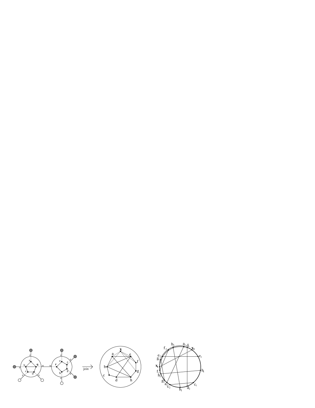
Figure 8: Example of insertion of $x$. The letters P, E, M stand for perfect, empty, mixed, respectively. The involved consecutivity preserving circle-join is the one illustrated in Figure 6.

Figure 8 provides an example of the insertion of a vertex $x$ to a circle graph $G$, where $N(x)=\{a,b,e,f,g\}$ and $G$ is described by the chord diagrams in Figures 5 and 6.

The construction applied in the proof of sufficiency for Theorem 3.11 is the basis of our circle graph recognition algorithm. Recall that successive circle-joins were applied to a path of labels in the split-tree, and each of these circle-joins preserved consecutiveness and bookends. The next section shows how that construction is used to recognize circle graphs.

4 Circle Graph Recognition Algorithm

We now have the material to present our circle graph recognition algorithm. It relies on the split decomposition algorithm of [15] and inserts the vertices one at a time according to an LBFS ordering $\sigma=x_{1}<\dots<x_{n}$. Implementation details from it that are needed for this paper will be introduced as required in the sections that follow. The reader should refer to [15] for complete implementation details.

For circle graph recognition, we will additionally need to maintain, at each prime node, a chord diagram. This is not required for degenerate nodes as their (potentially many) chord diagrams all have the same generic structure (see Figure 4). Whatever chord diagrams for degenerate nodes are required by the algorithm will be constructed as needed.

We first briefly describe how the split decomposition algorithm of [15] updates the split-tree of a graph under a vertex insertion. Based on this, we outline the vertex insertion test for circle graph recognition and prove its correctness. The data-structure and complexity issues are postponed to Section 5.

4.1 Incremental Modification of the Split-Tree

This subsection summarizes the general algorithm from [15]. The next subsection details specific cases and features of that algorithm that will be modified for the purposes of recognizing circle graphs.

We say that a node $u$ in a GLT (marked with respect to some set of leaves $S$) is hybrid if every marker vertex $q\in V(u)$ is either perfect or empty, and its opposite is mixed. A fully-mixed subtree $T^{\prime}$ of a GLT $(T,\mathcal{F})$ is a subtree of $T$ such that: it contains at least one tree-edge; the two extremities of all its tree-edges are mixed; and it is maximal for inclusion with respect to these properties. For a degenerate node $u$, we denote:

$$P^{*}(u) = \{q\in V(u)\mid q\textrm{ perfect and not the centre of a star}\},$$

$$E^{*}(u) = \{q\in V(u)\mid q\textrm{ empty, or }q\textrm{ perfect and the centre of a star}\}.$$

Theorem 4.1 (Theorem 4.14 in [15]).

Let $ST(G)=(T,\mathcal{F})$ be marked with respect to a subset $S$ of leaves. Then exactly one of the following conditions holds:

1. $ST(G)$ contains a clique node $u$ whose marker vertices are all perfect, and this node is unique;

2. $ST(G)$ contains a star node $u$ whose marker vertices are all empty except the centre, which is perfect, and this node is unique;

3. $ST(G)$ contains a unique hybrid node $u$ and this node is prime;

4. $ST(G)$ contains a unique hybrid node $u$ and this node is degenerate;

5. $ST(G)$ contains a tree-edge $e$ whose extremities are both perfect and this edge is unique;

6. $ST(G)$ contains a tree-edge $e$ with one extremity perfect and the other empty and this edge is unique;

7. $ST(G)$ contains a unique fully-mixed subtree $T$.

Now, for a new vertex $x$, and letting $S=N(x)$, the way $ST(G)$ has to be modified to obtain $ST(G+x)$ can be described as follows.

• If one of cases 1, 2 and 3 of Theorem 4.1 holds, then $ST(G+x)$ is obtained by adding to $u$ a marker vertex $q$ adjacent in $G(u)$ to precisely $P(u)$ and making the leaf $x$ the opposite of $q$.

• If case 4 of Theorem 4.1 holds, then $ST(G+x)$ is obtained in two steps:

  1. performing the node-split corresponding to $(P^{*}(u),E^{*}(u))$, thus creating a tree-edge $e$, the extremities of which are perfect or empty;

  2. subdividing $e$ with a new ternary node $v$ adjacent to $x$ and $e$’s extremities, such that $v$ is a clique if both extremities of $e$ are perfect, and otherwise $v$ is a star whose centre is the opposite of $e$’s empty extremity.

• If case 5 of Theorem 4.1 holds, then $ST(G+x)$ is obtained by subdividing $e$ with a new clique node adjacent to $e$’s extremities and $x$.

• If case 6 of Theorem 4.1 holds, then $ST(G+x)$ is obtained by subdividing $e$ with a new star node adjacent to $e$’s extremities and $x$, such that the centre of the star is opposite $e$’s empty extremity.

• If case 7 of Theorem 4.1 holds, then $ST(G+x)$ is obtained in three steps:

  1. [cleaning step] performing, for every degenerate node $u$ of $T$ the node-splits defined by $(P^{*}(u),V(u)\setminus P^{*}(u))$ and/or $(E^{*}(u),V(u)\setminus E^{*}(u))$ as soon as they are splits of $G(u)$. The resulting GLT is denoted $c\ell(ST(G))$, for cleaned split-tree.

  2. [contraction step] contracting, by a series of node-joins, the fully-mixed subtree of $c\ell(ST(G))$ into a single node $u$;

  3. [insertion step] adding to node $u$ a marker vertex $q_{x}$, adjacent in $G(u)$ to precisely $P(u)$, and making $q_{x}$ opposite $x$. The resulting node $u$ is prime.

This combinatorial charaterization of $ST(G+x)$ from $ST(G)$ is valid with no assumption on $x$. The split decomposition algorithm in [15] applies this characterization but inserts vertices with respect to an LBFS ordering because doing so allows its efficient implementation.

4.2 Incremental Circle Graph Recognition Algorithm

Here we describe how to refine the general construction described in Subsection 4.1 for the purposes of recognizing circle graphs. Let us repeat again that, while inserting vertices according to an LBFS ordering, we maintain the split-tree of the input graph as in [15] and with each prime node we associate a chord diagram. Let $G$ be a circle graph, and for a new vertex $x$, let $S=N(x)$. We consider how the changes to $ST(G)$ in arriving at $ST(G+x)$ necessitate updates to the chord diagrams being maintained at prime nodes.

• If one of cases 1, 2, 4, 5 or 6 of Theorem 4.1 holds, then the changes to $ST(G)$ amount to updating a degenerate node or creating a new degenerate node. By Corollary 2.19, this has no impact on the circle graph recognition problem. These modifications will therefore be handled by the split decomposition algorithm as described in [15].

• Case 3 of Theorem 4.1 amounts to updating a prime node $u_{x}$ by attaching a new leaf to it. In other words, adding a new vertex to the prime circle graph $G(u_{x})$ yields a new prime graph. We need to check whether this new prime graph is a circle graph as well. As the vertex insertion ordering is an LBFS ordering, the necessary and sufficient condition is that the neighbourhood of the new vertex is consecutive in the chord diagram of $G(u_{x})$ (Theorem 3.11 and Lemma 2.15).

• The core of the circle graph recognition algorithm resides in case 7 of Theorem 4.1. When $ST(G)$ contains a fully-mixed subtree, a new prime node is built in $ST(G+x)$ from existing nodes of $ST(G)$.

  The first step in case 7, namely the cleaning step, works as in the split-tree algorithm of [15]. It produces the GLT $cl(ST(G))$, the fully-mixed tree that will be transformed, in the second step, into a single node by means of all possible node-join operations. If $u_{x}$ is the result of the above node-joins, then let $G(u_{x})+x$ be the prime graph obtained in the third step by adding a vertex (corresponding to $x$) to $G(u_{x})$ with neighbourhood $P(u_{x})$.

  Notice the similarity between the node-joins in the second step and the construction in the proof of sufficiency of Theorem 3.11. In order to apply that theorem, we make the following observation:

  the fully-mixed subtree of $cl(ST(G))$, as considered in [15], corresponds canonically to $ST(G(u_{x}))$, as considered in Section 3.4 for $G=G(u_{x})$.

  We bring this to the attention of the reader because the implementation in [15] does not explicitly compute $G(u_{x})$ nor $ST(G(u_{x}))$. Instead, by the equivalence above, they exist implicitly as the fully-mixed portion of $cl(ST(G))$. We choose to ignore this technicality in what follows, instead using $ST(G(u_{x}))$ to refer to the fully-mixed portion of $cl(ST(G))$. We will take for granted that we have a data-structure encoding of $ST(G(u_{x}))$ by virtue of the data-structure encoding of $cl(ST(G))$ guaranteed by [15]. This equivalence will be recalled later as $cl(ST(G))\rightsquigarrow ST(G(u_{x}))$. The advantage of working with $ST(G(u_{x}))$ is that it allows for the direct application of Theorem 3.11.

  We apply Theorem 3.11 as follows. Prior to the node-joins in the second step, we test whether its conditions are satisfied for $ST(G(u_{x}))$. This can be done one node at a time. (In case of failure, the graph $G(u_{x})+x$ is not a circle graph, and thus neither is $G+x$.) More precisely, for each node $u$ containing a mixed marker vertex, we test whether $G(u)$ has a chord diagram $C_{u}$ in which $MP(u)$ is consecutive with mixed marker vertices being bookends. If the test does not fail, then we proceed as follows.

  During the contraction step, in addition to a series of node-joins made by algorithm [15] to contract the fully-mixed subtree, we perform a corresponding series of circle-joins, just as in the proof of sufficiency of Theorem 3.11. For two nodes $u$ and $v$ to be joined to form the new node $w$, we need to perform the circle-join that preserves the consecutiveness and bookends of $MP(u)$ and $MP(v)$ (Lemma 3.3).

  Finally, for the third step in case 7, the two endpoints representing a chord $c$ have to be inserted in the chord diagram $C_{u_{x}}$ of the node $u_{x}$ resulting from the contraction step. This new chord corresponds to $x$ and has to cross the chords of $P(u_{x})$. The result is a chord diagram for the new prime node labelled with $G(u_{x})+x$.

The vertex insertion procedure for circle graphs that is informally outlined above is captured more precisely as Algorithm 2. The correctness of Algorithm 2 follows from the above discussion, but we prove it more formally in Theorem 4.2 below. We point out that the implementation of this algorithm has to be thought of as complementary to the implementation from [15]. Thus, in order to lighten Algorithm 2, we consider that a node, whose label is a circle graph, may be directly labelled by a chord diagram of this circle graph.

Input: A graph $G$, a vertex $x\notin V(G)$ which is the last vertex in an LBFS ordering of $G+x$, and the split-tree $ST(G)=(T,\mathcal{F})$ equipped with chord diagrams on prime nodes.

Output: The split-tree $ST(G+x)$ equipped with chord diagrams on prime nodes, if $G+x$ is a circle graph.

1Determine which case of Theorem 4.1 applies based on algorithm [15];

2if case 1, 2, 4, 5 or 6 of Theorem 4.1 applies then

       update $ST(G)$ according to the algorithm [15], as described in Subsection 4.1;

      

3if case 3 of Theorem 4.1 applies (let $u_{x}$ be the unique hybrid prime node) then

      4 if $MP(u_{x})$ is consecutive in the chord diagram $C_{u_{x}}$ of $u_{x}$ (Theorem 3.11) then

             let $S$ be the factor of the chord diagram $C_{u_{x}}$ certifying the consecutiveness of $MP(u_{x})$;

            5 insert in $C_{u}$ a chord $c$ with endpoints $c_{1}$ and $c_{2}$ such that $C_{u_{x}}(c_{1},c_{2})=S$;

             add a leaf $x$ adjacent to $u_{x}$ opposite the marker vertex corresponding to chord $c$;

            

       else return $G+x$ is not a circle graph;

      ;

      

6if case 7 of Theorem 4.1 applies then

       compute $c\ell(ST(G))$ according to the algorithm [15] as described in Subsection 4.1;

       foreach tree-edge $uv$ of the fully-mixed subtree of $c\ell(ST(G))\rightsquigarrow ST(G(u_{x}))$ the extremities of which are $q_{u}$ and $q_{v}$ (they are mixed)  do

            7 if $u$, (respectively $v$) is degenerate then

                  if $G(u)$ (respectively $G(v)$) has a chord diagram in which $MP(u)$ is consecutive with mixed marker vertices being bookends then

                         build such a chord diagram $C_{u}$, respectively $C_{v}$

                   else return $G+x$ is not a circle graph;

                  ;

                  

            8 if $MP(u)$ is consecutive in $C_{u}$ with mixed marker vertices being bookends and $MP(v)$ is consecutive in $C_{v}$ with mixed marker vertices being bookends (Theorem 3.11) then

                  9 perform a circle-join between $C_{u}$ and $C_{v}$ with respect to $q_{u}$ and $q_{v}$ that preserves consecutiveness and bookends (Lemma 3.3);

                   consider that $u$ and $v$ are replaced with a single node whose chord diagram is the above resulting one;

                  

             else return $G+x$ is not a circle graph;

            ;

            

       end foreach

      let $C_{u_{x}}$ be the chord diagram of the node $u_{x}$ resulting from the series of circle-joins;

       let $S$ be the factor of the chord diagram $C_{u_{x}}$ certifying the consecutiveness of $P(u_{x})$;

      10 insert in $C_{u_{x}}$ a chord $c$ with endpoints $c_{1}$ and $c_{2}$ such that $C_{u_{x}}(c_{1},c_{2})=S$;

       add a leaf $x$ adjacent to $u_{x}$ opposite the marker vertex corresponding to chord $c$;

      

Algorithm 2 Vertex insertion

Theorem 4.2.

Given the split-tree $ST(G)$ of a circle graph, equipped with a chord diagram at every prime node, and given a good vertex $x$ of $G+x$, Algorithm 2 tests whether $G+x$ is a circle graph. If so, it returns $ST(G+x)$, equipped with a chord diagram at every prime node.

Proof.

Let $\sigma$ be an LBFS ordering of $G+x$ in which $x$ is good. The algorithm follows the vertex incremental construction of the split-tree proved in [15]. So if $G+x$ is a circle graph, then the returned GLT is its split-tree $ST(G+x)$. To prove the correctness of the recognition test, we focus on case 7, the other cases are straightforward. Let us consider the GLT $(T^{\prime},\mathcal{F^{\prime}})$ obtained from $ST(G)$ by contracting the fully-mixed subtree of $c\ell(ST(G))$ into a single node $u_{x}$ labelled by a graph $G(u_{x})$. Observe that $ST(G+x)$ is obtained from $(T^{\prime},\mathcal{F^{\prime}})$ by: (1) attaching $x$ as a leaf adjacent to node $u_{x}$; and (2) adding a new marker vertex $q_{x}$, opposite to leaf $x$ and adjacent to $S=P(u_{x})$ in $G(u_{x})$. It is proved in [15], that the resulting node $u^{\prime}$ and thereby the graph $G(u^{\prime})=G(u_{x})+q_{x}$ is prime.

As $G$ is a circle graph, $G(u_{x})$ is also a circle graph, by Corollary 2.19. Likewise, it is clear from Corollary 2.19 that $G+x$ is a circle graph if and only if $G(u^{\prime})$ is a circle graph. Also, by Lemma 2.15, $\sigma_{u^{\prime}}$ is an LBFS ordering of $G(u^{\prime})$ and thus $q_{x}$ is a good vertex of $G(u^{\prime})$. We apply Theorem 3.11 to $G(u_{x})$ (a circle graph), $G(u^{\prime})=G(u_{x})+q_{x}$ (a prime graph), and $q_{x}$ (a good vertex vertex). By doing so, we conclude that $G(u^{\prime})$ is prime if and only if for every node $v^{\prime}$ of $ST(G(u_{x}))$ marked with respect to $S$, $G_{v^{\prime}}$ has a chord diagram in which $MP(v^{\prime})$ is consecutive with mixed marker vertices being bookends. Now observe that, by construction, $ST(G(u_{x}))$ is isomorphic to the fully-mixed subtree $T_{m}$ of $c\ell(ST(G))$. We can thereby conclude that $G+x$ is a circle graph if and only if for every node $v$ of $T_{m}$, $G(v)$ has a chord diagram in which $MP(v)$ is consecutive with mixed marker vertices being bookends. Algorithm 2 precisely performs all these tests.

Now assume that $G+x$ is a circle graph. So as above, for every node $v$ of the fully-mixed subtree of $c\ell(ST(G))$, there exists a chord diagram $C_{v}$ in which $MP(v)$ is consecutive with mixed marker vertices being bookends. By Lemma 3.3, for every tree-edge $e=vw$ of $T_{m}$ with extremities $q_{v}\in V(v)$ and $q_{w}\in V(w)$, there is a circle-join of $C_{v}$ and $C_{w}$ with respect to $q_{v}$ and $q_{w}$ that preserves the consecutiveness and bookends. So eventually Algorithm 2 builds a chord diagram $C_{u_{x}}$ of node $u_{x}$ (to which $T_{m}$ is contracted) such that $MP(u_{x})=P(u_{x})$ is consecutive. Adding the chord $q_{x}$, corresponding to the marker vertex opposite $x$, yields a chord diagram of $G(u^{\prime})$ (which is prime). Therefore every prime node of $ST(G+x)$ is equipped with a chord diagram. ∎

Remark 4.3.

At two places in Algorithm 2 there seem to be possible choices, all leading to a final chord diagram: at line 2 to build a chord diagram of a degenerate node, whose existence (but not unicity) is guaranteed by assumption, and at line 2 to perform a circle-join, whose existence (but not unicity) is guaranteed by Lemma 3.3. In fact, since we obtain a chord diagram of a prime circle graph, known to be unique up to reflection, we know that, each time, there is a unique possible choice up to reflection.

5 Data-structure, Implementation and Running Time

The incremental split-tree algorithm from [15] can be implemented as described therein; it runs in time $O(n+m)\alpha(n+m)$. We mention that linear time LBFS implementations appear in [22] (see also [16]) and [17], and either of these can be used as part of the implementation for [15]. Thus, it remains to implement the routines involved in Algorithm 2: consecutiveness test on prime and degenerate nodes; construction of chord diagrams for degenerate nodes; circle-join operations preserving consecutiveness; and finally, chord insertion. To that aim, we first describe the data-structure used to maintain a chord diagram at each prime node of the split-tree throughout its construction. We then describe how Algorithm 2 can be implemented in order to obtain the $O(n+m)\alpha(n+m)$ time complexity for the circle graph recognition problem.

5.1 Chord Diagram Data-Structure

We introduce a new data structure for chord diagrams, namely consistent symmetric cycles, see below. At first glance it would seem that the usual and natural data-structure for chord diagrams would be a circular doubly-linked list; unfortunately, this choice would not allow the performance we require. In particular, under such a data-structure each endpoint would be represented by a node with two pointers, say prev and next, pointing to the endpoint’s counter-clockwise and clockwise neighbours, respectively, in the chord diagram. This would allow consecutive sets of endpoints to be efficiently located and circle-joins to be efficiently performed. The problem is that our circle graph recognition algorithm sometimes performs circle joins using the reflection of a chord diagram. In a circular, doubly-linked list, this would require updating all the prev pointers to become next pointers and vice versa. That proves too costly. To achieve the desired running time for circle graph recognition, circle-joins must be performed in constant time.

One constant-time circle-join alternative using circular, doubly-linked lists would be to simply reinterpret prev as next and vice versa without actually reassigning pointers. But this becomes a problem when the circle-join is performed between one chord diagram, say $C$, and the reflection of another, say $C^{\prime r}$. In that case, pairs of next pointers will end up pointing to each other and pairs of prev pointers will end up pointing to each other. Figure 6 provides one example of a circle-join where this would happen. In that case, the traditional procedure for traversing a circular, doubly-linked list would no longer work. Some of the next and prev pointers need to be interpreted as normal (those from $C$) while the other ones need to be interpreted as the opposite (those from $C^{\prime r}$). The data structure we propose below for chord diagrams generalizes the circular, doubly-linked list to allow for this duality.

Definition 5.1.

A symmetric cycle is the digraph $C$ obtained from a cycle by replacing every edge with a pair of opposite arcs. Every vertex $y$ of a symmetric cycle is thereby associated with two out-neighbours, namely $+_{C}(y)$ and $-_{C}(y)$.

Definition 5.2.

Let $C$ be a symmetric cycle on the vertex set ${\mathcal{V}}=\bigcup_{v\in{\mathcal{V}}}\{v_{1},v_{2}\}$. Then each $v_{1},v_{2}$ are said to be matched, and $C$ is said to be consistent if for every pair $y_{1}$ and $y_{2}$ of matched vertices, $+_{C}(y_{1})$ and $+_{C}(y_{2})$ belong to the same connected component of $C-\{y_{1},y_{2}\}$.

Our data-structure for a chord diagram on $V$ implements in the natural way a consistent symmetric cycle (CSC) on ${\mathcal{V}}=\cup_{v\in V}\{v_{1},v_{2}\}$. That is, for a chord $y\in V$, the two endpoints $y_{1}$ and $y_{2}$ are matched with pointers from each one to the other. Pointers are also maintained between $y$ and those endpoints. Observe that a CSC for chord diagram $C$ is simultaneously a CSC for chord diagram $C^{r}$. One can distinguish a chord diagram and its reflection by specifying a direction. That is, precisely: chord diagrams up to reflection are encoded by CSCs, and chord diagrams are encoded by CSCs together with the choice of a direction. In what follows, we assume that this precision is implicit and we will just talk about CSCs as encoding chord diagrams. This data-structure is illustrated in Figure 9. Observe that searching a CSC in a given direction is achieved in linear time by a depth-first search (DFS).

Figure 9: Example encoding of a circle graph by a CSC. Arrows represent pointers. The $+/-$ pointer types in the CSC structure are distinguished by two types of dashed arrows. The consistency rule for these pointers is illustrated on the right.

Let $y_{1}$ and $y_{2}$ be the endpoints of chord $y$ of the chord diagram $C$. Let $+_{C}(y_{1},y_{2})$ denote the sequence of endpoints (other than $y_{1}$ and $y_{2}$) encountered while starting a DFS on $C$ from $y_{1}$ with pointer $+_{C}(y_{1})$ and stopping at $+_{C}(y_{2})$. The sequences $-_{C}(y_{1},y_{2})$, $+_{C}(y_{2},y_{1})$ and $-_{C}(y_{2},y_{1})$ are defined similarly. Observe that the sequence $+_{C}(y_{1},y_{2})$ is the reversal of $+_{C}(y_{2},y_{1})$. The following observation establishes the links between the CSC representation of a chord diagram $C$ and its representation by a circular word.

Observation 5.3.

If $y_{1}$ and $y_{2}$ are the endpoints of chord $y$ in a chord diagram $C$, then exactly one of the following holds:

1. $+_{C}(y_{1},y_{2})=C(y_{1},y_{2})$ (and thus $+_{C}(y_{2},y_{1})=C^{r}(y_{1},y_{2})$, $-_{C}(y_{1},y_{2})=C^{r}(y_{2},y_{1})$ and $-_{C}(y_{2},y_{1})=C(y_{2},y_{1})$)

2. $+_{C}(y_{1},y_{2})=C^{r}(y_{2},y_{1})$ (and thus $+_{C}(y_{2},y_{1})=C(y_{2},y_{1})$, $-_{C}(y_{1},y_{2})=C(y_{1},y_{2})$ and $-_{C}(y_{2},y_{1})=C^{r}(y_{1},y_{2})$)

For the sake of implementation, this data-structure for circle graphs completes the data-structure used in [15] to represent the split-tree $ST(G)$ of a graph $G$.

5.2 Implementation with CSCs

This section uses CSCs to implement the routines involved in Algorithm 2 and evaluates their costs. The computation of the perfect/empty/mixed states for marker vertices of nodes is handled in the algorithm from [15] (here at line 2 in Algorithm 2). Notably, the set of non-empty marker vertices $MP(u)$ is also computed by [15], and assumed to be known for every involved node $u$. It is also important to remind the reader that a CSC simultaneously encodes a chord diagram $C$ and its reflection $C^{r}$. This will be crucial for the efficiency of the implementation of Algorithm 2.

5.2.1 Testing Consecutiveness in a CSC

There are three different times during algorithm 2 when we need to test whether $G(u)$ has a chord diagram $C_{u}$ in which the chords of $MP(u)$ are consecutive with mixed marker vertices being bookends (lines 2, 2 and 2). We also have to build such a chord diagram if the node is degenerate (line 2 in Algorithm 2). Recall that a prime label is already equipped with its chord diagram. We argue below that, if $u$ is a degenerate node, then this test can be performed (and a chord diagram can be built) in constant time; and otherwise, this test can be performed in $O(|MP(u)|)$.

The case of degenerate nodes follows directly from Theorem 3.10, satisfied by $ST(G(u_{x}))$.

Lemma 5.4.

Let $ST(G)$ be marked with respect to $N(x)$ with $x$ a good vertex of $G+x$. If $u$ is a degenerate node of the fully-mixed subtree of $c\ell(ST(G))$ $\rightsquigarrow ST(G(u_{x}))$, then testing if there exists a CSC for a chord diagram $C_{u}$ of $G(u)$ in which $MP(u)$ is consecutive with mixed marker vertices being bookends, and, if so computing it, requires constant time.

Proof.

Assume there exists a chord diagram $C_{u}$ in which $MP(u)$ is consecutive with mixed marker vertices being bookends. Therefore $MP(u)$ contains at most two mixed marker vertices. Applying Theorem 3.10 to $ST(G(u_{x}))$, we see that $u$ has at most two non-mixed marker vertices. Hence, $u$ contains at most four marker vertices. The number of possible chord diagrams is thereby bounded by a constant (there are at most 8 chord endpoints to arrange). Thus, the construction of an appropriate chord diagram $C_{u}$, or the test that no appropriate chord diagram exists, can be done in constant time. Let us recall that chord diagrams of degenerate nodes have the form demonstrated in Figure 4. ∎

We now consider the case of a prime node $u$. Recall that the set $MP(u)$ is given, as well as a chord diagram $C_{u}$ of $G(u)$ (in fact unique up to reflection).

Lemma 5.5.

Let $ST(G)$ be marked with respect to $N(x)$ with $x$ a good vertex of $G+x$. If $u$ is a prime node, then testing if $MP(u)$ is consecutive with mixed marker vertices being bookends in the chord diagram $C_{u}$ of $G(u)$ requires $O(|MP(u)|)$ time.

Proof.

Recall that $MP(u)$ can be assumed to have been computed by the split algorithm of [15]. Consider some marker vertex $q\in MP(u)$. If $S_{e}$ is a set of endpoints certifying that $MP(u)$ is consecutive in $C_{u}$, then $q_{1}\in S_{e}$ or $q_{2}\in S_{e}$ but not both. Moreover, $S_{e}$ is of the form $S_{e}^{-}q_{1}S_{e}^{+}$ or $S_{e}^{-}q_{2}S_{e}^{+}$ with $S_{e}^{-}$ and $S_{e}^{+}$ being possibly empty words. So, to test the consecutiveness of $MP(u)$, it suffices to test the existence of these sets $S_{e}^{-}$ and $S_{e}^{+}$ of endpoints. To that aim, proceed as follows: search $C_{u}$ from $q_{1}$ in one direction, say using the pointer $-_{C_{u}}(q_{1})$, as long as the encountered endpoint corresponds to a marker vertex $q^{\prime}$ of $MP(u)$ and the other endpoint of $q^{\prime}$ has not yet been discovered. Using the pointers between the endpoints of each chord, it can be determined in constant time if the other endpoint has already been discovered. Perform the same search in the other direction, i.e. with the pointer $+_{C_{u}}(q_{1})$. If $S_{e}^{-}q_{1}S_{e}^{+}$ isn’t located in this, then perform the same search, but this time starting at $q_{2}$. With these searches, the existence of $S_{e}$ can be determined in $O(|MP(u)|)$ time with DFS. Once this test has been performed, testing if non-bookend elements of $S$ are non-mixed has the same cost $O(|MP(u)|)$. ∎

5.2.2 Circle-Joins Preserving Consecutiveness (with CSCs)

We want to prove that we can identify – in constant time – which of the four possible circle-joins of Lemma 3.3 preserves consecutiveness and bookends (line 2 in Algorithm 2). Recall that some of the constructions from Lemma 3.3 use the reflection of the chord diagram. Our use of consistent symmetric cycles and their property of being invariant under reflection (Section 5.1) is important in this regard: it means that no additional work is required to compute the reflection of a chord diagram in implementing the circle-joins of Lemma 3.3.

Lemma 5.6.

Let $C_{u}$ and $C_{v}$ be two chord diagrams, respectively, on the set of chords $V(u)$ and $V(v)$. Let $S_{u}\subseteq V(u)$ and $S_{v}\subseteq V(v)$ be consecutive sets of chords in $C_{u}$ and $C_{v}$, respectively. Given the CSCs for $C_{u}$ and $C_{v}$, the bookends $q$ and $q^{\prime}$ of $S_{u}$, and the bookends $r$ and $r^{\prime}$ of $S_{v}$, one can build in constant time a CSC for a chord diagram $C$ on $(V(u)\setminus\{q\})\cup(V(v)\setminus\{r\})$ satisfying the conclusion of Lemma 3.3, which we recall as

1. $C$ results from a circle-join $\odot$ or $\hat{\odot}$ of $C_{u}$ and $C_{v}$ or $C^{r}_{v}$ with respect to $q$ and $r$,

2. $S=(S_{u}\setminus\{q\})\cup(S_{v}\setminus\{r\})$ is consecutive in $C$,

3. $S$ has bookends $q^{\prime}$ and $r^{\prime}$.

Proof.

We will address the following case (the others are similar): $C_{u}(q_{1},q^{\prime}_{1})$ and $C_{v}(r_{1},r^{\prime}_{1})$ respectively certify the consecutiveness of $S_{u}$ in $C_{u}$ and of $S_{v}$ in $C_{v}$; $C_{u}(q_{1},q^{\prime}_{1})$ and $C_{v}(r_{1},r^{\prime}_{1})$ are, respectively, strictly contained in $C_{u}(q_{1},q_{2})$ and $C_{v}(r_{1},r_{2})$; $C_{u}(q_{1},q_{2})=+_{C_{u}}(q_{1},q_{2})$ and $C_{v}(r_{1},r_{2})=+_{C_{v}}(r_{1},r_{2})$. By Observation 5.3, we have

$(C_{u},q)\odot(C_{v},r)\sim+_{C_{u}}(q_{1},q_{2})+_{C_{v}}(r_{1},r_{2})-_{C_{u}}(q_{2},q_{1})-_{C_{v}}(r_{2},r_{1})$

$(C_{u},q)~{}\hat{\odot}~{}(C_{v},r)\sim+_{C_{u}}(q_{1},q_{2})-_{C_{v}}(r_{2},r_{1})-_{C_{u}}(q_{2},q_{1})+_{C_{v}}(r_{1},r_{2})$

$(C_{u},q)\odot(C^{r}_{v},r)\sim+_{C_{u}}(q_{1},q_{2})-_{C_{v}}(r_{1},r_{2})-_{C_{u}}(q_{2},q_{1})+_{C_{v}}(r_{2},r_{1})$

$(C_{u},q)~{}\hat{\odot}~{}(C^{r}_{v},r)\sim+_{C_{u}}(q_{1},q_{2})+_{C_{v}}(r_{2},r_{1})-_{C_{u}}(q_{2},q_{1})-_{C_{v}}(r_{1},r_{2})$

By Lemma 3.3, one of the four chord diagrams above preserves consecutiveness and bookends. Under the assumptions above, $S$ is consecutive in $C=(C_{u},q)~{}\hat{\odot}~{}(C^{r}_{v},r)$, with bookends $r^{\prime}$ and $q^{\prime}$. The CSC for $C$ is obtained from those for $C_{u}$ and $C_{v}$ by reassigning a constant number of pointers. For example, assuming the following (the other cases are similar):

$-_{C_{u}}(q_{1})=a_{u}$ and $+_{C_{u}}(a_{u})=q_{1}$; $+_{C_{u}}(q_{1})=b_{u}$ and $-_{C_{u}}(b_{u})=q_{1}$;

$+_{C_{u}}(q_{2})=c_{u}$ and $+_{C_{u}}(c_{u})=q_{2}$; $-_{C_{u}}(q_{2})=d_{u}$ and $+_{C_{u}}(d_{u})=q_{2}$;

$-_{C_{v}}(r_{1})=a_{v}$ and $+_{C_{v}}(a_{v})=r_{1}$; $-_{C_{v}}(r_{1})=b_{v}$ and $-_{C_{v}}(b_{v})=r_{1}$;

$-_{C_{v}}(r_{2})=c_{v}$ and $+_{C_{v}}(c_{v})=r_{2}$; $-_{C_{v}}(r_{2})=d_{v}$ and $+_{C_{v}}(d_{v})=r_{2}$;

then we perform the following updates:

$+_{C}(b_{v})=b_{u}$ and $-_{C}(b_{u})=b_{v}$; $+_{C}(c_{u})=a_{v}$ and $+_{C}(a_{v})=c_{u}$;

$+_{C}(d_{v})=d_{u}$ and $+_{C}(d_{u})=d_{v}$; $+_{C}(a_{u})=c_{v}$ and $+_{C}(c_{v})=a_{u}$.

It is not difficult to check that the above pointer reassignments preserve the consistency property. Regarding the running time, observe that only a constant number of pointer reassignments are required. Moreover, given the bookends $q_{1},q_{1}^{\prime},r_{1},r_{1}^{\prime}$, their other endpoints $q_{2},q_{2}^{\prime},r_{2},r_{2}^{\prime}$, respectively, can be accessed in constant time using the pointers between the endpoints of each chord. And to decide in constant time which of the possible circle-joins we need to perform, it suffices to store a constant size table describing every possible case, along with the required circle-join operation for that case. ∎

5.2.3 Chord Insertion in a CSC

To complete the implementation of Algorithm 2, it remains to describe how a new chord $c$ can be inserted in a CSC. This task occurs at lines 2 and 2. In both cases the resulting chord diagram $C$ corresponds to a prime graph. Moreover, thanks to the previous steps, the neighbourhood of the vertex represented by $c$ is consecutive in $C$.

Lemma 5.7.

Given a CSC for a chord diagram $C$ and the bookends of a consecutive set $S_{e}$ of endpoints in $C$, the insertion of a new chord $c$ intersecting exactly the chords with an endpoint in $S_{e}$ requires constant time.

Proof.

Let $b$ and $b^{\prime}$ be the bookends of $S_{e}$ and let $a\notin S_{e}$ and $a^{\prime}\notin S_{e}$ be the endpoints neighbouring $b$ and $b^{\prime}$, respectively. It suffices to reassign a constant number of pointers towards the endpoints $c_{1}$ and $c_{2}$ of the new chord $c$. For example, if $+_{C}(a)=b$ and $+_{C}(b)=a$, then set $+_{C}(a)=c_{1}$ and $+_{C}(b)=c_{1}$; and if $-_{C}(b^{\prime})=a$ and $+_{C}(a^{\prime})=b^{\prime}$, then set $-_{C}(b^{\prime})=c_{2}$ and $+_{C}(a^{\prime})=c_{2}$. The other cases are symmetric. Following that, we need to initialize the pointers of $c_{1}$ and $c_{2}$ in a consistent way: for example $+_{C}(c_{1})=b$ and $+_{C}(c_{2})=b^{\prime}$. ∎

5.3 The Running Time

As already described, compared to the LBFS incremental split decomposition algorithm of [15], the circle graph recognition problem must only handle the consecutiveness test of Algorithm 2 and the maintenance of CSCs for the chord diagrams of prime nodes. So if we prove that, at each vertex insertion, these tasks can be performed in time linear in the cost of the split-tree modifications, then we could conclude that the circle graph recognition problem can be solved as efficiently as the split decomposition algorithm. Regarding the latter, [15] proved the following:

Theorem 5.8 (Theorem 6.21 in [15]).

The split-tree $ST(G)$ of a graph $G=(V,E)$ with $n$ vertices and $m$ edges can be built incrementally according to an LBFS ordering in time $O(n+m)\alpha(n+m)$, where $\alpha$ is the inverse Ackermann function.

For an LBFS ordering $\sigma=x_{1}<\dots<x_{n}$ of a graph $G$, let $G_{i}$ be the subgraph of $G$ induced by $V_{i}=\{x_{1},\dots,x_{i}\}$. Let insertion-cost$(x_{i},ST(G_{i-1}))$ denote the complexity of the LBFS incremental split decomposition algorithm [15] to compute $ST(G_{i})$ from $ST(G_{i-1})$ marked with $N_{i}(x_{i})=N(x_{i})\cap V_{i-1}$. From Theorem 5.8 we have:

$$\sum_{i=1}^{n}\mbox{{insertion-cost}}(x_{i},ST(G_{i-1}))~{}\in~{}O(n+m)\alpha(n+m)$$

Theorem 5.9.

The circle graph recognition test can be performed in time $O(n+m)\alpha(n+m)$ on any graph on $n$ vertices and $m$ edges.

Proof.

Let $\sigma=x_{1}<\dots<x_{n}$ be an LBFS ordering of the graph $G$. Assume that $ST(G_{i-1})$, marked with respect to $N_{i}(x_{i})$, is equipped with a CSC at every prime node. We prove that computing $ST(G_{i})$ and the CSCs of its prime nodes (if $G_{i}$ is a circle graph) requires $O($insertion-cost$(x_{i},$ $ST(G_{i-1})))$.

First, observe that in cases 1, 2, 4, 5, and 6 of Theorem 4.1 (line 2 in Algorithm 2) the prime nodes of $ST(G_{i-1})$ are not affected by $x_{i}$’s insertion. So none of the CSCs stored at prime nodes are affected, and thus no extra work is required for the circle graph recognition problem.

Now assume that case 3 of Theorem 4.1 holds (line 2 in Algorithm 2). Let $u_{x}$ denote the unique prime hybrid node of $ST(G_{i-1})$. We need to insert a chord $c$ in the CSC for the chord diagram $C_{u_{x}}$ of $G(u_{x})$ which exactly intersects the chords in $MP(u_{x})$. As $u_{x}$ is the only prime node affected by $x_{i}$’s insertion (Theorem 3.11), $G_{i}$ is a circle graph if and only if $MP(u_{x})$ is consecutive in $C_{u_{x}}$. As $ST(G_{i-1})$ is marked with respect to $N_{i}(x_{i})$ (i.e. $MP(u_{x})$ is identified by the split-tree algorithm), testing the consecutiveness of $MP(u_{x})$ requires $O(|MP(u_{x})|)$ time, by Lemma 5.5. Moreover by Lemma 5.7, inserting the chord $c$ only takes constant time. The total amount of time spent to update the CSC for $C_{u_{x}}$ is clearly $O($insertion-cost$(x_{i},ST(G_{i-1})))$, since $MP(u_{x})$ has been computed by the split decomposition tree algorithm (at this step $i$).

Finally, assume that case 7 of Theorem 4.1 holds (line 2 in Algorithm 2). Let $u_{x}$ denote the node resulting from the contraction of the fully-mixed subtree $T_{m}$ of $c\ell(ST(G_{i-1}))$ $\rightsquigarrow ST(G(u_{x}))$. We need to compute a CSC for the chord diagram $C_{u_{x}}$ of $G({u_{x}})$ such that $MP({u_{x}})$ is consecutive and then insert a new chord, say $c_{x}$, exactly intersecting $MP({u_{x}})$. Again, by Theorem 3.11, this is possible (i.e. $G_{i}$ is a circle graph) if and only if every node $v$ of $T_{m}$ has a chord diagram in which $MP(v)$ is consecutive with mixed marker vertices being bookends. This property of $MP(v)$ can be tested and built in constant time if $v$ is a degenerate node of $c\ell(ST(G_{i-1}))$ (Lemma 5.4), and can be tested in $O(|MP(v)|)$ time if $v$ is a prime node of $T_{m}$ (by Lemma 5.5). The sum of these costs over involved nodes $v$ is $O($insertion-cost$(x_{i},ST(G_{i-1})))$ since $MP(v)$ is computed by the split decomposition algorithm [15] for each $v$. Moreover, by Lemma 5.6, with a constant time extra cost, a circle-join preserving consecutiveness and bookends can be performed in parallel to every node-join operation required to contract $T_{m}$ into ${u_{x}}$ that is performed by the split decomposition algorithm [15], with total cost $O($insertion-cost$(x_{i},ST(G_{i-1})))$. Finally as in the previous case, we eventually insert the new chord $c_{x}$ in the CSC for the resulting chord diagram $C_{u_{x}}$. By Lemma 5.7, this also requires constant time since $MP({u_{x}})$ is known. In total, the amount of time spent to built the CSC of the new prime node is $O($insertion-cost$(x_{i},ST(G_{i-1})))$. ∎

6 Concluding Remarks

This paper presents the first subquadratic circle graph recognition algorithm. It also develops a new characterization of circle graphs in terms of LBFS (upon which the algorithm is based). The algorithm operates incrementally, extending the incremental split decomposition algorithm from the companion paper [15]. The two operate in parallel. As each new vertex is inserted, the circle graph recognition algorithm inspects properties of the split-tree to determine if the resulting graph will remain a circle graph. If it does, the split-tree is updated to account for the new vertex. The running time for the entire process is $O(n+m)\alpha(n+m)$, where $\alpha$ is the inverse Ackermann function, which is essentially constant for all practical graphs. It is important to note that this $\alpha$ factor is due to the split decomposition algorithm; the circle portion is consistent with linear time. Thus, a linear time implementation of the split decomposition portion would result in a linear time circle graph recognition algorithm.

Eliminating the dependence on the incremental split decomposition portion may prove difficult. Recall that split decomposition reduces the problem of recognizing circle graphs to that of recognizing prime circle graphs. But since prime graphs cannot be further decomposed, simply knowing the split decomposition a priori does not help. Therefore bypassing the incremental split decomposition portion above may necessarily mean bypassing split decomposition altogether. In this way, it is necessary to fully explore the implications of the new LBFS characterization. Being specified in terms of LBFS end vertices, it appears uniquely suited to the incremental setting of this paper. It remains to be seen if it can be applied to some benefit in the “offline” setting. Linear time circle graph recognition via the LBFS characterization could still be a possibility with such an approach.

But there may yet be additional applications of the incremental split decomposition algorithm coupled with the LBFS characterization. One possibility for exploration is rank-width determination. Its connection with circle graphs was noted in the introduction. However, there are also connections with split decomposition. For example, distance-hereditary graphs – the family of graphs without prime subgraphs – are precisely the graphs with rank-width 1. An algorithm to determine the split decomposition of distance-hereditary graphs appeared in [13, 14] using a restricted version of the algorithm presented in our companion paper. It would be interesting to investigate what LBFS and split decomposition can together reveal about other graphs of bounded rank-width. Similarly, could LBFS and split decomposition yield fast simple recognition algorithms for permutation graphs (strictly contained in circle graphs) as well as parity graphs and Meyniel graphs? Both families strictly contain distance-hereditary graphs.

References

- [1] A. Bouchet. Reducing prime graphs and recognizing circle graphs. Combinatorica, 7:243–254, 1987.
- [2] A. Bouchet. Graphic presentations of isotropic systems. Journal of Combinatorial Theory, Series B, 45:58–76, 1988.
- [3] T. H. Cormen, C. Stein, R.L. Rivest, and C.E. Leiserson. Introduction to Algorithms. McGraw-Hill Higher Education, 2001.
- [4] D.G. Corneil. Lexicographic breadth first search - a survey. In International Workshop on Graph Theoretical Concepts in Computer Science (WG), Lecture Notes in Computer Science, 3353:1–19, 2004.
- [5] B. Courcelle. The monadic second-order logic of graphs XVI: canonical graph decomposition. Logical Methods in Computer Science, 2(2):1–46, 2006.
- [6] B. Courcelle. Circle graphs and monadic second-order logic. Journal of Applied Logic, 6(3):416 – 442, 2008.
- [7] W.H. Cunningham. Decomposition of directed graphs. SIAM Journal on Algebraic Discrete Methods, 3:214–228, 1982.
- [8] E. Dahlhaus. Parallel algorithms for hierarchical clustering and applications to split decomposition and parity graph recognition. Journal of Algorithms, 36(2):205–240, 2000.
- [9] F. Dragan, F. Nicolai, and A. Brandstädt. LexBFS-orderings and powers of graphs. In International Workshop on Graph Theoretical Concepts in Computer Science (WG), Lecture Notes in Computer Science, 1197:166–180, 1996.
- [10] S. Even and A. Itai. Queues, stacks and graphs. Theory of Machines and Computations, pages 71–86, 1971.
- [11] C.P. Gabor, W.L. Hsu, and K.J. Suppovit. Recognizing circle graphs in polynomial time. Journal of ACM, 36:435–473, 1989.
- [12] J. Geelen and S.-I. Oum. Circle graph obstructions under pivoting. Journal of Graph Theory,, 61(1):1–11, 2009.
- [13] E. Gioan and C. Paul. Dynamic distance hereditary graphs using split decomposition. In International Symposium on Algorithms and Computation (ISAAC), Lecture Notes in Computer Science, 4835:41–51, 2007.
- [14] E. Gioan and C. Paul. Split decomposition and graph-labelled trees: characterizations and fully-dynamic algorithms for totally decomposable graphs. Discrete Applied Mathematics, 160(6):708–733, 2012.
- [15] E. Gioan, C. Paul, M. Tedder, and D. Corneil. Practical and efficient split decomposition via graph-labelled trees. arXiv:1104.3283, 2011.
- [16] M.C. Golumbic. Algorithmic graph theory and perfect graphs, 2nd Edition. Elsevier, 2004.
- [17] M. Habib, R.M. McConnell, C. Paul, and L. Viennot. Lex-BFS and partition refinement, with applications to transitive orientation, interval graph recognition and consecutive ones testing. Theoretical Computer Science, 234, 1-2: 59-84, 2000.
- [18] T.-H. Ma and J. Spinrad. An algorithm for undirected split decomposition. Journal of Algorithms, 16:145–160, 1994.
- [19] W. Naji. Reconnaissance des graphes de cordes. Discrete Mathematics, 54:329–337, 1985.
- [20] S.-I. Oum. Rank-width and vertex minors. Journal of Combinatorial Theory, Series B, 95(1):79–100, 2005.
- [21] S.-I. Oum. Excluding a bipartite circle graph from line graphs. Journal of Graph Theory, 60(3):183–203, 2009.
- [22] D.J. Rose, R.E. Tarjan, and G.S. Lueker. Algorithmic aspects of vertex elimination on graphs. SIAM Journal on Computing, 5(2):266–283, 1976.
- [23] J. Spinrad. Recognition of circle graphs. Journal of Algorithms, 16:264–282, 1994.
- [24] R.E. Tarjan. Efficiency of a good but not linear set union algorithm. Journal of the ACM, 22(2):146–160, 1975.