Affine trajectory correction for
nonholonomic mobile robots

Abstract

Planning trajectories for nonholonomic systems is difficult and computationally expensive. When facing unexpected events, it may therefore be preferable to deform in some way the initially planned trajectory rather than to re-plan entirely a new one. We suggest here a method based on affine transformations to make such deformations. This method is exact and fast: the deformations and the resulting trajectories can be computed algebraically, in one step, and without any trajectory re-integration. To demonstrate the possibilities offered by this new method, we use it to derive position and orientation correction algorithms for the general class of planar wheeled robots and for a tridimensional underwater vehicle. These algorithms allow in turn achieving more complex applications, including obstacle avoidance, feedback control or gap filling for sampling-based kinodynamic planners.

I Introduction

A bicycle, a car, an aircraft, or a submarine are but a few examples of nonholonomic systems. Planning trajectories for such systems is difficult because, by nature, some of their degrees of freedom can only be controlled in a coupled manner (see e.g. [13] and references therein). As a consequence, when such systems encounter on their ways an unexpected event (e.g. a random perturbation of the system state or of the target state, an unforeseen obstacle, etc.), it may be more efficient to deform in some manner the initially planned trajectory rather than to re-plan entirely a new one [11, 10, 12, 19].

Lamiraux and colleagues [12] suggested to iteratively deform the original path by perturbing infinitesimally the control inputs at each iteration. However, as underlined by Seiler and colleagues [19], that method requires re-integrating the whole trajectory at each iteration, which is computationally expensive. These authors then described a new method based on Lie group symmetries, which requires re-integrating only parts of the trajectory.

The Lie groups considered in [4, 19] are in fact Euclidean (or isometry) groups. We propose here to use larger Lie groups, namely, affine groups, which contain the Euclidean transformations as subgroups. Using affine transformations allows making more versatile trajectory corrections. In particular, the corrections are exact and can be computed algebraically, in one step, which makes iterative deformations [12] or gradient search [4, 19] unnecessary. Furthermore, there is no need to re-integrate even a part of the trajectory. Note that, in contrast with previous works where the studied systems are invariant under Euclidean transformations [4, 19], here trajectories and control inputs are not in general affine-invariant. More technical precautions need therefore to be taken to define and guarantee the feasibility (or admissibility) of the deformed trajectories under the system nonholonomic constraints. In particular, the admissibility conditions are formulated using differential equations with discontinuous right-hand sides [5].

In section II, we present the general framework of affine trajectory correction. We then apply this framework to derive position and orientation correction algorithms for two classical examples in nonholonomic mobile robotics: the general class of planar wheeled robots (sections III) and a tridimensional underwater vehicle (section IV). In section V, we study some more elaborate applications including trajectory correction for a car towing trailers, obstacle avoidance, feedback control and gap-filling techniques. Finally, in section VI, we discuss the advantages and drawbacks of the presented method, its domain of applicability, and possible future developments.

A preliminary version [17] of the present manuscript describing position and orientation correction algorithms for the unicycle, the bicycle and an underwater vehicle was accepted for presentation at the conference Robotics: Science and Systems 2011.

II General framework

II-A Affine spaces and affine transformations

An affine space is a set $\mathbb{A}$ together with a group action of a vector space $\mathbb{W}$. An element $\mathbf{w}\in\mathbb{W}$ transforms a point $P\in\mathbb{A}$ into another point $P^{\prime}$ by $P^{\prime}=P+\mathbf{w},$ which can also be noted $\overrightarrow{PP^{\prime}}=\mathbf{w}$.

Given a point $O\in\mathbb{A}$ (the origin), an affine transformation $\mathcal{F}$ of the affine space can be defined by a couple $(\mathbf{w},\mathcal{M})$ where $\mathbf{w}\in\mathbb{W}$ and $\mathcal{M}$ is a non-singular endomorphism of $\mathbb{W}$ (i.e. a non-singular linear application $\mathbb{W}\rightarrow\mathbb{W}$). The transformation $\mathcal{F}$ operates on $\mathbb{A}$ by

$$\forall P\in\mathbb{A}\quad\mathcal{F}(P)=O+\mathcal{M}(\overrightarrow{OP})+\mathbf{w}.$$

Note that, if $P_{0}$ is a fixed-point of $\mathcal{F}$, then $\mathcal{F}$ can be written in the form

$$\forall P\in\mathbb{A}\quad\mathcal{F}(P)=P_{0}+\mathcal{M}(\overrightarrow{P_{0}P}).$$

II-B Admissible trajectories and admissible trajectory deformations

Let us consider a commanded system of dimension $N$. Suppose that $n$ of the system variables form an affine space. As an example, consider the unicycle model [13]

$$\left\{\begin{array}[]{ccc}\dot{x}&=&v\cos(\theta)\\ \dot{y}&=&v\sin(\theta)\\ \dot{\theta}&=&\omega\end{array}\right.,$$ (1)

where $(v,\omega)$ are the system control inputs (or commands) and $(x,y,\theta)$, the system variables. The $(x,y)$ space can be viewed as an affine space of dimension $n=2$. We call $(x,y)$ the base variables and the associated affine space, the base space.

We say that a full-space trajectory $\bar{\mathcal{C}}(t)_{t\in[0,T]}$ ($\bar{\mathcal{C}}(t)=(x(t),y(t),\theta(t))$ in the above example) is admissible if one can find a set of admissible commands ($v$ and $\omega$ in the example) that generates $\bar{\mathcal{C}}$. A base-space trajectory $\mathcal{C}$ ($\mathcal{C}=(x,y)$ in the example) is admissible if there exists an admissible full-space trajectory whose projection on the base space coincides with $\mathcal{C}$.

Let $\mathcal{C}(t)_{t\in[0,T]}$ be a base-space trajectory and $\tau\in[0,T]$, a given time instant. We say that a transformation $\mathcal{F}$ occurring at $\tau$ deforms $\mathcal{C}(t)_{t\in[0,T]}$ into $\mathcal{C}^{\prime}(t)_{t\in[0,T]}$ if

$$\begin{array}[]{rcl}\forall t<\tau&{}\hfil&\mathcal{C}^{\prime}(t)=\mathcal{C}(t)\\ \forall t\geq\tau&{}\hfil&\mathcal{C}^{\prime}(t)=\mathcal{F}(\mathcal{C}(t)).\end{array}$$

Given an admissible base-space trajectory $\mathcal{C}$, an affine transformation $\mathcal{F}$ is said to be admissible if $\mathcal{F}$ deforms $\mathcal{C}$ into an admissible trajectory.

II-C Differential equations with discontinuous right-hand sides

For convenience, we denote by $\mathscr{D}^{0}$ the space of piecewise continuous functions with finite limits at the discontinuity points – or piecewise $C^{0}$ functions (see Fig. 1, top plot, for an example). Typically, the linear acceleration of a mobile robot would belong $\mathscr{D}^{0}$: indeed, any brusque press on the throttle or on the brake pedal would correspond to a discontinuity of the linear acceleration.

Figure 1: Examples of functions of $\mathscr{D}^{0}$ (top) and of $\mathscr{D}^{1}$ (bottom). Note that the top function is actually the derivative of the bottom function.

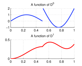
Let $u$ be a function of $\mathscr{D}^{0}$ and consider the following differential equation with discontinuous right-hand side (see [5])

$$\left\{\begin{array}[]{rcl}\dot{x}(t)&=&u(t)\\ x(0)&=&x_{0}\\ \end{array}\right..$$ (2)

It follows from the definition of $\mathscr{D}^{0}$ that any solution $x$ of system (2) is $C^{0}$ and piecewise $C^{1}$. Conversely, for any function $x$ which is $C^{0}$ and piecewise $C^{1}$, one has $\dot{x}\in\mathscr{D}^{0}$. For convenience, we denote by $\mathscr{D}^{1}$ the space of such $x$ functions (see Fig. 1, bottom plot, for an example).

Finally, we denote by $\mathscr{D}^{2}$ the space of differentiable functions whose derivatives are in $\mathscr{D}^{1}$. This definition does not involve technical difficulties since the functions of $\mathscr{D}^{1}$ are continuous.

In the unicycle example of section II-B, if the linear and angular accelerations $a$ and $\omega$ are assumed to be in $\mathscr{D}^{0}$ then the linear velocity $v$ and the orientation $\theta$ will belong to $\mathscr{D}^{1}$, which implies in turn that the position $(x,y)$ belongs to $\mathscr{D}^{2}$.

II-D Dimension of the space of admissible affine deformations

From the previous section, one can see that, typically, some of the variables are required to be continuous. These continuity conditions are particularly critical at the time instant $\tau$ when the deformation occurs. In general, if one needs to guarantee the continuities of $m$ variables at $\tau$, this will define $m$ constraints on the set of admissible affine transformations. On the other hand, the affine transformations of an $n$-dimensional space form a Lie group of dimension $n+n^{2}$ ($n$ coordinates for the translation and $n^{2}$ coordinates for the endomorphism of the associated vector space, where $n$ is the number of base variables). Consequently, if $n+n^{2}>m$, one could expect to have at our disposal $\tau$ and $n+n^{2}-m$ “extra degrees of freedom” to achieve the desired correction while staying admissible.

For wheeled robots of class I (see section III-C) and wheeled robots of class II (section III-D), the base space $(x,y)$ is of dimension $n=2$. We show that there are respectively $m=4$ and $m=5$ continuity conditions for these systems, yielding respectively $n+n^{2}-m=2$ and $n+n^{2}-m=1$ “extra degrees of freedom”. We then suggest how to play with $\tau$ and these “extra degrees of freedom” to make corrections towards virtually any desired final position and orientation. For the tridimensional underwater vehicle (section IV), the base space $(x,y,z)$ is of dimension $n=3$ and there are $m=6$ continuity conditions, yielding $n+n^{2}-m=6$ “extra degrees of freedom”.

III Affine trajectory correction for planar wheeled robots

The above presented framework suggests the following general scheme to study affine trajectory correction for a particular system

1. check the conditions for a base-space trajectory to be admissible;

2. characterize the set of admissible affine deformations;

3. compute the admissible affine deformation that achieves the desired trajectory correction.

To illustrate, let us now apply the above scheme to wheeled robots, which constitute an important class of nonholonomic systems.

III-A Model description

At the kinematic level, any wheeled robot whose wheels obey the rolling without slipping constraints can be modeled by [3]

$$\left\{\begin{array}[]{ccl}\dot{\xi}&=&B(\xi,\beta)\eta\\ \dot{\beta}&=&\zeta\end{array}\right.$$

where $\xi=(x,y,\theta)^{\top}$ is the posture of the robot and $\beta=(\beta_{1}\dots\beta_{h})^{\top}$ contains the steering angles of the centered orientable conventional wheels ($h=0$ if there are no such wheels). As in the unicycle example of section II-B, we choose $x$ and $y$ to be the base variables. The base space is thus of dimension 2. The non-base variables are $\theta$ and $\beta_{1}\dots\beta_{h}$.

Throughout this section III, we assume, to avoid singularities, that the linear velocity $\sqrt{\dot{x}^{2}+\dot{y}^{2}}$ of the robot is always strictly positive.

The commands of the system are given by $\eta$, which contains the linear velocities of well-defined reference points on the frame of the robot, and $\zeta$, which contains the rates of change of the steering angles of the centered orientable wheels. We assume that the commands obey the following conditions

• the space of admissible commands $\eta$ is $\mathscr{D}^{1}$. This is consistent with the fact that the linear accelerations $a$ of the reference points, which are the derivatives of $\eta$, are in $\mathscr{D}^{0}$. The possible discontinuities of $a$ would correspond to e.g. brusque presses on the throttle or on the brake pedal;

• the space of admissible commands $\zeta$ is $\mathscr{D}^{0}$. The possible discontinuities of $\zeta$ would correspond to e.g. hard turns of the steering wheel in a car.

III-B Admissible base-space trajectories

As shown in [3], any planar wheeled mobile robot can be described by one out of the five sets of “forward” kinematic equations of Table I, given a suitable choice of a reference point and of a basis attached to the robot frame.

TABLE I: Forward and reverse kinematic equations for planar wheeled robots

Type	Examples	“Forward” kinematic equations (cf [3])	“Reverse” equations	Admissibility cond.
(3,0)	Omni- directional robots	$\begin{array}[]{ccl}(\dot{x},\dot{y})^{\top}&=&\mathbf{R}(\theta)(\eta_{1},\eta_{2})^{\top}\\ \dot{\theta}&=&\eta_{3}\end{array}$ where $\mathbf{R}(\theta)=\left(\begin{array}[]{cc}\cos\theta&-\sin\theta\\ \sin\theta&\cos\theta\end{array}\right)$	$\begin{array}[]{ccl}\theta&\in&\mathscr{D}^{2}\textrm{ (arbitrary)}\\ (\eta_{1},\eta_{2})^{\top}&=&\mathbf{R}(\theta)^{-1}(\dot{x},\dot{y})^{\top}\\ \eta_{3}&=&\dot{\theta}\end{array}$	$(x,y)\in\mathscr{D}^{2}$
(2,0)	Two-wheel differential drive	$\begin{array}[]{ccl}\dot{x}&=&-\eta_{1}\sin\theta\\ \dot{y}&=&\eta_{1}\cos\theta\\ \dot{\theta}&=&\eta_{2}\end{array}$	$\begin{array}[]{ccl}\theta&=&\mathrm{arctan2}(\dot{y},\dot{x})\\ \eta_{1}&=&\sqrt{\dot{x}^{2}+\dot{y}^{2}}\\ \eta_{2}&=&\dot{\theta}\end{array}$	$(x,y)\in\mathscr{D}^{2}$ $\mathrm{arctan2}(\dot{y},\dot{x})\in\mathscr{D}^{2}$
(2,1)	Unicycle	$\begin{array}[]{ccl}\dot{x}&=&-\eta_{1}\sin(\theta+\beta)\\ \dot{y}&=&\eta_{1}\cos(\theta+\beta)\\ \dot{\theta}&=&\eta_{2}\\ \dot{\beta}&=&\zeta_{1}\end{array}$	$\begin{array}[]{ccl}\theta&\in&\mathscr{D}^{2}\textrm{ (arbitrary)}\\ \beta&=&\mathrm{arctan2}(\dot{y},\dot{x})-\theta\\ \eta_{1}&=&\sqrt{\dot{x}^{2}+\dot{y}^{2}}\\ \eta_{2}&=&\dot{\theta}\\ \zeta_{1}&=&\dot{\beta}\end{array}$	$(x,y)\in\mathscr{D}^{2}$
(1,1)	Bicycle, kinematic car	$\begin{array}[]{ccl}\dot{x}&=&-\eta_{1}L\sin\theta\sin\beta\\ \dot{y}&=&\eta_{1}L\cos\theta\sin\beta\\ \dot{\theta}&=&\eta_{1}\cos\beta\\ \dot{\beta}&=&\zeta_{1}\end{array}$	$\begin{array}[]{ccl}\theta&=&\mathrm{arctan2}(\dot{y},\dot{x})\\ \beta&=&\mathrm{arctan2}(\dot{y}/(L\cos\theta),\dot{\theta})\\ \eta_{1}&=&\sqrt{\dot{x}^{2}+\dot{y}^{2}}/(L\sin\beta)\\ \zeta_{1}&=&\dot{\beta}\end{array}$	$(x,y)\in\mathscr{D}^{2}$ $\mathrm{arctan2}(\dot{y},\dot{x})\in\mathscr{D}^{2}$
(1,2)	Kludge robot (cf [3])	$\begin{array}[]{ccl}\dot{x}&=&-\eta_{1}(2L\cos\theta\sin\beta_{1}\sin\beta_{2}\\ &&+L\sin\theta\sin(\beta_{1}+\beta_{2}))\\ \dot{y}&=&-\eta_{1}(2L\sin\theta\sin\beta_{1}\sin\beta_{2}\\ &&-L\cos\theta\sin(\beta_{1}+\beta_{2}))\\ \dot{\theta}&=&\eta_{1}\sin(\beta_{2}-\beta_{1})\\ \dot{\beta}_{1}&=&\zeta_{1}\\ \dot{\beta}_{2}&=&\zeta_{2}\end{array}$	$\begin{array}[]{ccl}\theta&\in&\mathscr{D}^{2}\textrm{ (arbitrary)}\\ \beta_{1}&=&\mathrm{arctan2}(\dot{x}\cos\theta+\dot{y}\sin\theta,\\ &&2L\dot{\theta}-\dot{x}\sin\theta+\dot{y}\cos\theta)\\ \beta_{1}&=&\mathrm{arctan2}(\dot{x}\cos\theta+\dot{y}\sin\theta,\\ &&-2L\dot{\theta}-\dot{x}\sin\theta+\dot{y}\cos\theta)\\ \eta_{1}&=&\dot{\theta}/\sin(\beta_{2}-\beta_{1})\\ \zeta_{1}&=&\dot{\beta}_{1}\\ \zeta_{2}&=&\dot{\beta}_{2}\end{array}$	$(x,y)\in\mathscr{D}^{2}$

For each type of robot, we now characterize the admissible base-space trajectories given the spaces of admissible commands assumed in the previous section. The reader is referred to Table I for the necessary notations and equations.

III-B1 Type (3,0)

Consider $(\eta_{1},\eta_{2},\eta_{3})\in\mathscr{D}^{1}$. The third “forward” kinematic equation ($\dot{\theta}=\eta_{3}$) implies that $\theta\in\mathscr{D}^{2}$. The first and the second forward equations then imply that $x\in\mathscr{D}^{2}$ and $y\in\mathscr{D}^{2}$.

Conversely, consider a base-space trajectory $\mathcal{C}=(x,y)\in\mathscr{D}^{2}$. One can choose an arbitrary function $\theta\in\mathscr{D}^{2}$ and then compute $(\eta_{1},\eta_{2},\eta_{3})\in\mathscr{D}^{1}$ by the “reverse” equations.

In summary, a base-space trajectory of a (3,0) wheeled robot is admissible if and only if it belongs to $\mathscr{D}^{2}$.

III-B2 Type (2,0)

Consider $(\eta_{1},\eta_{2})\in\mathscr{D}^{1}$. As previously, the forward equations imply that $x$ and $y$ belong to $\mathscr{D}^{2}$.

Conversely, consider a base-space trajectory $\mathcal{C}=(x,y)\in\mathscr{D}^{2}$. One can then compute $\theta$ by the first reverse equation $\theta=\mathrm{arctan2}(\dot{y},\dot{x})$ where

$$\mathrm{arctan2}(b,a)=\left\{\begin{array}[]{cc}\pi/2&\textrm{if $a=0$ and $b\geq 0$}\\ -\pi/2&\textrm{if $a=0$ and $b<0$}\\ \arctan(b/a)&\textrm{if $a\neq 0$}\end{array}\right..$$

Remark that the so-calculated $\theta$ belongs to $\mathscr{D}^{1}$, but not necessarily to $\mathscr{D}^{2}$. Next, one can compute $\eta_{2}$ by the third reverse equation. For $\eta_{2}$ to be in $\mathscr{D}^{1}$, one would need $\theta\in\mathscr{D}^{2}$. As just remarked, the latter condition is not automatically guaranteed by $\mathcal{C}=(x,y)\in\mathscr{D}^{2}$. On the other hand, demanding that $\mathcal{C}=(x,y)\in\mathscr{D}^{3}$ would be unduly restrictive. Thus the condition $\theta\in\mathscr{D}^{2}$ must be specified as an independent supplementary condition.

In summary, a base-space trajectory $\mathcal{C}$ of a (2,0) robot is admissible if and only if it belongs to $\mathscr{D}^{2}$, and if the function $\theta$ – as computed from $\mathcal{C}$ by the first reverse equation – also belongs to $\mathscr{D}^{2}$.

Note that these admissibility conditions can also be formulated in terms of continuity constraints on the path curvature [2, 7].

III-B3 Type (2,1)

Consider $(\eta_{1},\eta_{2})\in\mathscr{D}^{1}$ and $\zeta\in\mathscr{D}^{0}$. The third and fourth forward equations imply that $\theta$ and $\beta$ belong respectively to $\mathscr{D}^{2}$ and $\mathscr{D}^{1}$. Next, the first and second forward equations imply that $x$ and $y$ belong to $\mathscr{D}^{2}$.

Conversely, consider a base-space trajectory $\mathcal{C}=(x,y)\in\mathscr{D}^{2}$. One can choose an arbitrary function $\theta\in\mathscr{D}^{2}$ and then compute successively $\beta\in\mathscr{D}^{1}$, $(\eta_{1},\eta_{2})\in\mathscr{D}^{1}$, and $\zeta\in\mathscr{D}^{0}$ by the reverse equations.

In summary, as for (3,0) robots, a base-space trajectory of a (2,1) robot is admissible if and only if it belongs to $\mathscr{D}^{2}$.

III-B4 Type (1,1)

As previously, a necessary condition for the admissibility of a base-space trajectory is that it belongs to $\mathscr{D}^{2}$. Conversely, consider $\mathcal{C}=(x,y)\in\mathscr{D}^{2}$. The first reverse equation allows to compute $\theta\in\mathscr{D}^{1}$. Remark that, as for $(2,0)$ robots, the so-calculated $\theta$ does not necessarily belong to $\mathscr{D}^{2}$. Next, $\beta$ can be computed from the second reverse equation. Remark that the derivative of $\theta$ is used in the computation of $\beta$, such that $\beta$ belongs to $\mathscr{D}^{0}$, but not necessarily to $\mathscr{D}^{1}$. However, in order to compute next $\zeta$, one needs $\beta\in\mathscr{D}^{1}$, and consequently $\theta\in\mathscr{D}^{2}$.

In summary, as for (2,0) robots, a base-space trajectory $\mathcal{C}$ of a (1,1) robot is admissible if and only if it belongs to $\mathscr{D}^{2}$, and if the function $\theta$ – as computed from $\mathcal{C}$ by the first reverse equation – also belongs to $\mathscr{D}^{2}$.

III-B5 Type (1,2)

This type of robots can be treated in the same way as (3,0) and (2,1) robots. A base-space trajectory of a (1,2) robot is admissible if and only if it belongs to $\mathscr{D}^{2}$.

III-B6 Summary

Following the previous development, one can divide wheeled robots in two classes. Class I comprises robots of type (3,0), (2,1), and (1,2), or in other words, those whose degrees of maneuvrability [3] equal 3. A base-space trajectory for robots of this class is admissible if and only if it belongs to $\mathscr{D}^{2}$.

Class II comprises robots of type (2,0) and (1,1), or in other words, those whose degrees of maneuvrability equal 2. A base-space trajectory $\mathcal{C}=(x,y)$ for robots of this class is admissible if and only if it belongs to $\mathscr{D}^{2}$ and if the function $\theta=\mathrm{arctan2}(\dot{y},\dot{x})$ also belongs to $\mathscr{D}^{2}$.

Important remark: From a computational viewpoint, if one obtains an admissible base-space trajectory $\mathcal{C}^{\prime}(t)_{t\in[0,T]}$ (for instance by deforming a given $\mathcal{C}(t)_{t\in[0,T]}$), the reverse equations allow to easily compute the commands that generate that trajectory by some differentiations and elementary operations. $\triangle$

Relationship with flatness theory: Our approach here bears some resemblance with flatness theory [6]. In both cases, a reduced set of variables is manipulated (here: the base variables; in flatness theory: the flat outputs) and the state of the other variables are subsequently recovered from this reduced set (here: using the reverse equations). There are however two important differences. First, in our approach, certain non-base variables, in some systems, are not computed from the base variables but chosen arbitrarily: e.g. the orientation $\theta$ in wheeled robots of class I (see above) or the roll angle $\phi$ in the underwater vehicle (see section IV-B). Second, in some systems, certain non-base variables are computed from the base variables using integration: e.g. the orientation $\theta_{i}$ ($i>0$) of the trailers (see section V-A). In flatness theory, all non-base variables must be computed from the flat outputs, and they must be done so using only differentiations and algebraic operations.

Finally, note that it could be interesting to study affine deformations of the trajectories of the flat outputs. $\triangle$

III-C Class I robots

We now characterize the affine deformations that preserve the admissibility of base-space trajectories for robots of class I. Using this characterization, we then suggest practical algorithms for trajectory correction.

III-C1 Admissible deformations

Consider an admissible base-space trajectory $\mathcal{C}(t)_{t\in[0,T]}$ and an affine deformation $\mathcal{F}$ occurring at time $\tau$ that deforms $\mathcal{C}$ into $\mathcal{C}^{\prime}$. In what follows, we note $v=\sqrt{\dot{x}^{2}+\dot{y}^{2}}$ (the linear velocity of the robot) and $\theta=\mathrm{arctan2}(\dot{y},\dot{x})$ (its orientation). Note that, following section III-B6, $\mathcal{C}$ is admissible if and only if $(x,y)\in\mathscr{D}^{2}$, i.e., if and only if $(v,\theta)\in\mathscr{D}^{1}$. Note also that the function $\theta$ here is not the same as the $\theta$ chosen arbitrarily in Table I. For instance, the unicycle described by equations (1) is a in fact a (2,1) robot, with the following correspondance between the variables

$$\left\{\begin{array}[]{ccc}\theta_{\mathrm{robot}}&=&0\\ \beta_{\mathrm{robot}}&=&\theta_{\mathrm{unicycle}}-\pi/2\\ {\eta_{1}}_{\mathrm{robot}}&=&v_{\mathrm{unicycle}}\\ {\eta_{2}}_{\mathrm{robot}}&=&0\\ \zeta_{\mathrm{robot}}&=&\omega_{\mathrm{unicycle}}\end{array}\right..$$ (3)

One has first, by definition, $\mathcal{C}^{\prime}(t)_{t\in(\tau,T]}=\mathcal{F}(\mathcal{C}(t)_{t\in(\tau,T]})$. Since $\mathcal{F}$ is a smooth application, it is clear that $\mathcal{C}^{\prime}(t)_{t\in(\tau,T]}$ – note that the interval is open at $\tau$ – is in $\mathscr{D}^{2}$ if and only if $\mathcal{C}(t)_{t\in(\tau,T]}$ is in $\mathscr{D}^{2}$.

Regarding the time instant $\tau$, the continuities of $x$ and $y$ impose that $\mathcal{F}(\mathcal{C}(\tau))=\mathcal{C}(\tau)$. Thus $\mathcal{F}$ can be written in the form

$$\forall P\in\mathbb{A}\quad\mathcal{F}(P)=\mathcal{C}(\tau)+\mathcal{M}(\overrightarrow{\mathcal{C}(\tau)P}).$$ (4)

One now needs to guarantee the continuities of $v$ and $\theta$ at $\tau$, since the two remaining conditions (differentiability and finite limits for the derivative) do not depend on the behavior of $\mathcal{C}^{\prime}$ at the discrete point $\tau$, and are therefore already satisfied by virtue of the smoothness of $\mathcal{F}$.

Consider the velocity vector $\mathbf{v}=(\dot{x},\dot{y})^{\top}$. Remark that the continuity of this velocity vector is equivalent to those of $v$ and $\theta$. The continuity of $\mathbf{v}$ means that $\mathbf{v}(\tau-)$ and $\mathbf{v}(\tau+)$ (where the signs $-$ and $+$ denote respectively the left and right limits) are well defined, and that $\mathbf{v}(\tau-)=\mathbf{v}(\tau+)=\mathbf{v}(\tau)$.

Similarly, the continuity of $\mathbf{v}^{\prime}$ would mean $\mathbf{v}^{\prime}(\tau+)=\mathbf{v}^{\prime}(\tau-)=\mathbf{v}(\tau)$. On the other hand, one has $\mathbf{v}^{\prime}(\tau+)=\mathcal{M}(\mathbf{v}(\tau))$. These equalities together imply $\mathcal{M}(\mathbf{v}(\tau))=\mathbf{v}(\tau)$.

Let us now decompose $\mathcal{M}$ is the basis $\{\mathbf{u}_{\parallel},\mathbf{u}_{\perp}\}$ where $\mathbf{u}_{\parallel}=(\cos(\theta),\sin(\theta))^{\top}$ is the unit tangent vector and $\mathbf{u}_{\perp}=(-\sin(\theta),\cos(\theta))^{\top}$ is the unit normal vector. The condition $\mathcal{M}(\mathbf{v}(\tau))=\mathbf{v}(\tau)$ is equivalent to

$$\exists\lambda,\mu\in\mathbb{R}\quad\mathbf{M}=\left(\begin{array}[]{rcl}1&\lambda\\ 0&1+\mu\end{array}\right),$$ (5)

where $\mathbf{M}$ is the matrix representing $\mathcal{M}$ in the basis $\{\mathbf{u}_{\parallel},\mathbf{u}_{\perp}\}$.

In summary, the admissible affine transformations at time $\tau$ form a Lie group of dimension 2, parameterized by $\lambda$ and $\mu$ in equation (5)

III-C2 Trajectory correction

We consider only the correction of the final position and assume that $\tau$ is given. It is possible to achieve more complex corrections (e.g. correcting the final orientation) or to choose “optimal” $\tau$s: these developments are left to the reader.

From equation (4), to correct the final position $\mathcal{C}(T)$ towards a desired position $P_{d}=(x_{d},y_{d})$, one needs to look for a linear application $\mathcal{M}$ such that

$$\mathcal{M}(\overrightarrow{\mathcal{C}(\tau)\mathcal{C}(T)})=\overrightarrow{\mathcal{C}(\tau)P_{d}}.$$ (6)

Let $\mathbf{Q}=[\mathbf{u}_{\|},\mathbf{u}_{\perp}]$ and let the matrix representing $\mathcal{M}$ in the basis $\{\mathbf{u}_{\|},\mathbf{u}_{\perp}\}$ be

$$\mathbf{M}=\left(\begin{array}[]{cc}1&\lambda\\ 0&1+\mu\\ \end{array}\right).$$

Equation (6) implies

$$\mathbf{Q}\mathbf{M}\mathbf{Q}^{-1}\left(\begin{array}[]{c}x(T)-x(\tau)\\ y(T)-y(\tau)\\ \end{array}\right)=\left(\begin{array}[]{c}x_{d}-x(\tau)\\ y_{d}-y(\tau)\\ \end{array}\right).$$ (7)

Let next

$$\left(\begin{array}[]{c}x_{1}\\ y_{1}\\ \end{array}\right)=\mathbf{Q}^{-1}\left(\begin{array}[]{c}x(T)-x(\tau)\\ y(T)-y(\tau)\\ \end{array}\right),$$

$$\left(\begin{array}[]{c}x_{2}\\ y_{2}\\ \end{array}\right)=\mathbf{Q}^{-1}\left(\begin{array}[]{c}x_{d}-x(\tau)\\ y_{d}-y(\tau)\\ \end{array}\right).$$

Equation (7) then implies

$$\lambda=(x_{2}-x_{1})/y_{1},\quad\mu=(y_{2}-y_{1})/y_{1},$$

provided that $y_{1}\neq 0$, i.e. that the tangent at $\tau$ does not go through $\mathcal{C}(T)$ (see also discussion in section III-D2). Fig. 8 shows examples of trajectory corrections for the unicycle.

Note that any desired position in the whole space – and not only those in the vicinity of the initially planned final position as in [19] – can theoretically be reached. Remark on the other hand that the distance (e.g. the $L_{2}$ distance) of the corrected trajectory from the original trajectory is a continuous function of $\lambda$ and $\mu$, meaning that using small $\lambda$s and $\mu$s results in small changes in the overall trajectory (and in the commands).

III-D Class II robots

III-D1 Admissible deformations

Consider an admissible base-space trajectory $\mathcal{C}$ of a class II robot and an affine deformation $\mathcal{F}$ occurring at time $\tau$ that deforms $\mathcal{C}$ into $\mathcal{C}^{\prime}$. In what follows, we note $v=\sqrt{\dot{x}^{2}+\dot{y}^{2}}$ (the linear velocity of the robot), $\theta=\mathrm{arctan2}(\dot{y},\dot{x})$ (its orientation), and $\omega=\dot{\theta}$ (its angular velocity). Note that, following section III-B6, $\mathcal{C}$ is admissible if and only if $v\in\mathscr{D}^{1}$ and $\omega\in\mathscr{D}^{1}$.

Following the same reasoning as in section III-C1, one can show that $\mathcal{C}^{\prime}(t)_{t\in(\tau,T]}$ is in $\mathscr{D}^{2}$ if and only if $\mathcal{F}(\mathbf{v}(\tau))=\mathbf{v}(\tau)$, where $\mathbf{v}(\tau)$ is is the velocity vector at $\tau$. One now needs to check the continuities of $\omega^{\prime}$ at $\tau$ and at the discontinuity points of the second derivative of $\mathcal{C}$ (the continuity and differentiability of $\omega^{\prime}$ elsewhere are already guaranteed by the smoothness of $\mathcal{F}$, cf. section III-C1).

Consider for this the acceleration vector $\mathbf{a}=(\ddot{x},\ddot{y})^{\top}$. By definition, one has

$$\mathbf{a}=a\mathbf{u}_{\parallel}+v\omega\mathbf{u}_{\perp},$$

with $\mathbf{a}$ not necessarily continuous. One can next write

$$\mathbf{a}\cdot\mathbf{u}_{\perp}=v\omega.$$ (8)

Consider now a time instant $t>\tau$ when $\mathbf{a}$ is possibly discontinuous, that is $\mathbf{a}(t-)\neq\mathbf{a}(t+)$. Since $\omega$ and $v$ are continuous, one has by equation (8)

$$\mathbf{a}(t-)\cdot\mathbf{u}_{\perp}(t)=\mathbf{a}(t+)\cdot\mathbf{u}_{\perp}(t),$$

or, in other words, that $\mathbf{a}(t+)-\mathbf{a}(t-)$ and $\mathbf{u}_{\parallel}(t)$ are collinear. Here comes into play a nice property of affine transformations: they preserve collinearity. Using this property, one obtains that $\mathcal{M}(\mathbf{a}(t+)-\mathbf{a}(t-))$ and $\mathcal{M}(\mathbf{u}_{\parallel}(t))$ are collinear. But the former vector is no other than $\mathbf{a}^{\prime}(t+)-\mathbf{a}^{\prime}(t-)$ and the latter is collinear with $\mathbf{u}^{\prime}_{\parallel}(t)$, since

$$\mathbf{u}^{\prime}_{\parallel}(t)=\frac{\mathcal{M}(\mathbf{u}_{\parallel}(t))}{\|\mathcal{M}(\mathbf{u}_{\parallel}(t))\|}.$$

Thus $\mathbf{a}^{\prime}(t-)\cdot\mathbf{u}^{\prime}_{\perp}(t)=\mathbf{a}^{\prime}(t+)\cdot\mathbf{u}^{\prime}_{\perp}(t)$, which in turn implies the continuity of $\omega^{\prime}$ at $t$ (note that this conclusion also relies on the fact that $v^{\prime}$ is nonzero if $v$ is nonzero, owing to the non-singularity of $\mathcal{M}$).

Remark: Since the affine group is the largest transformation group of the plane that preserves collinearity, the previous development shows that it is also the largest group that preserves the admissibility of every trajectory of a class II robot! $\triangle$

Turning now to the time instant $\tau$, the same reasoning as previously shows that $\omega^{\prime}$ is continuous at $\tau$ if and only if

$$\mathbf{a}^{\prime}(\tau+)\cdot\mathbf{u}_{\perp}(\tau)=\mathbf{a}(\tau)\cdot\mathbf{u}_{\perp}(\tau),$$

or equivalently, if

$$\mathcal{M}(\mathbf{a}(\tau))\cdot\mathbf{u}_{\perp}(\tau)=\mathbf{a}(\tau)\cdot\mathbf{u}_{\perp}(\tau).$$ (9)

Remark now that, since $\mathbf{v}\cdot\mathbf{u}_{\perp}=0$, condition (9) is in fact equivalent to

$$\exists\lambda\in\mathbb{R}\quad\mathcal{M}(\mathbf{a}(\tau))=\mathbf{a}(\tau)+\lambda\mathbf{v}(\tau).$$

Denoting by $\mathcal{B}$ the linear application such that $\mathcal{B}(\mathbf{v}(\tau))=\mathbf{0}$ and $\mathcal{B}(\mathbf{a}(\tau))=\mathbf{v}(\tau)$ (one can compute $\mathcal{B}$ explicitly by $\mathcal{B}=[\mathbf{0},\mathbf{v}(\tau)][\mathbf{v}(\tau),\mathbf{a}(\tau)]^{-1}$), one obtains

$$\exists\lambda\in\mathbb{R}\quad\mathcal{M}=\mathcal{I}+\lambda\mathcal{B},$$

where $\mathcal{I}$ is the identity application.

In summary, the admissible affine transformations at time $\tau$ form a Lie group of dimension 1, given by $\{\mathcal{I}+\lambda\mathcal{B}\}_{\lambda\in\mathbb{R}}$.

Inflection points: The previous development is valid only when $\mathbf{v}(\tau)$ and $\mathbf{a}(\tau)$ are non-collinear, that is, when $\mathcal{C}(\tau)$ is not an inflection point (see also [1] for an interesting discussion on inflection points in the context of human movements). $\triangle$

III-D2 Trajectory correction I: position correction using one affine deformation

Let us now play with $\tau$ and the “extra degree of freedom” $\lambda$ to make trajectory corrections.

For this, we first study how the final position of the trajectory $\mathcal{C}(T)$ is affected by an admissible affine deformation occurring at time $\tau$. By definition, one has

$$\begin{array}[]{rcl}\mathcal{C}^{\prime}(T)&=&\mathcal{C}(\tau)+(\mathcal{I}+\lambda\mathcal{B})(\overrightarrow{\mathcal{C}(\tau)\mathcal{C}(T)})\\ &=&\mathcal{C}(T)+\lambda\mathcal{B}(\overrightarrow{\mathcal{C}(\tau)\mathcal{C}(T)}).\end{array}$$

Let us decompose $\overrightarrow{\mathcal{C}(\tau)\mathcal{C}(T)}$ in the (in general non-orthonormal) basis $\{\mathbf{v}(\tau),\mathbf{a}(\tau)\}$

$$\overrightarrow{\mathcal{C}(\tau)\mathcal{C}(T)}=\gamma\mathbf{v}(\tau)+\delta\mathbf{a}(\tau).$$

By definition of $\mathcal{B}$, one has

$$\mathcal{C}^{\prime}(T)=\mathcal{C}(T)+\lambda\delta\mathbf{v}(\tau).$$ (10)

Consequently, if $\delta$ is nonzero (that is, if $\overrightarrow{\mathcal{C}(\tau)\mathcal{C}(T)}$ and $\mathbf{v}(\tau)$ are non-collinear, or in other words, if the tangent at $\tau$ does not go through $\mathcal{C}(T)$), then the locus of $\mathcal{C}^{\prime}(T)$ when $\lambda$ varies is the line that goes through $\mathcal{C}(T)$ and that collinear with $\mathbf{v}(\tau)$.

In order to make a correction of the final position from $\mathcal{C}(T)$ to a desired position $P_{d}$, it therefore suffices to

1. compute the vector $\mathbf{e}_{d}=\overrightarrow{\mathcal{C}(T)P_{d}}$;

2. find a time instant $\tau$ when the tangent $\mathbf{u}_{\parallel}(\tau)$ is collinear with $\mathbf{e}_{d}$;

3. compute $\lambda=\overline{\mathbf{e}_{d}}/(\delta\overline{\mathbf{v}(\tau)})$ where the overline denotes the signed norm;

4. make the affine deformation of parameter $\lambda$ at time $\tau$.

Fig. 2 shows some examples of trajectory correction for a kinematic car, which is a robot of type (1,1). The equation of a kinematic car is given by [13]

$$\left\{\begin{array}[]{ccc}\dot{x}&=&v\cos(\theta)\\ \dot{y}&=&v\sin(\theta)\\ \dot{\theta}&=&\frac{v\tan(\beta)}{L}\\ \dot{\beta}&=&\zeta\\ \end{array}\right.,$$ (11)

which can be put in the form of a robot of type (1,1) (cf. Table I) using the following correspondance between the variables

$$\left\{\begin{array}[]{ccc}\theta_{\mathrm{robot}}&=&\theta_{\mathrm{car}}-\pi/2\\ \beta_{\mathrm{robot}}&=&\pi/2-\beta_{\mathrm{car}}\\ {\eta_{1}}_{\mathrm{robot}}&=&v_{\mathrm{car}}/(L\cos\beta_{\mathrm{car}})\\ \zeta_{\mathrm{robot}}&=&-\zeta_{\mathrm{car}}\end{array}\right..$$ (12)

Figure 2: Accessible final positions (in cyan) and two examples of position corrections. The original trajectory is in red. For each correction, the black plain line represents the tangent at $\tau$ while the black dotted line joins the original final position $\mathcal{C}(T)$ to the desired final position $P_{d}$. Note the collinearity of the plain line and the dotted line.

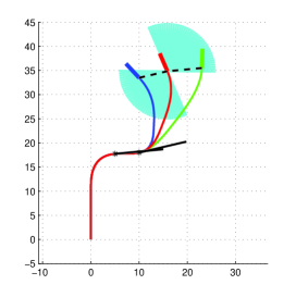
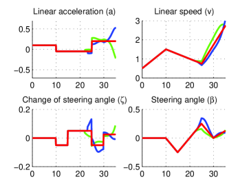
Accessible positions: From the previous development, it appears that a position $P_{d}$ is accessible if and only if the original trajectory $\mathcal{C}(t)_{t\in[0,T]}$ has a tangent that is parallel to $\overrightarrow{\mathcal{C}(T)P_{d}}$. Therefore the set of the trajectory tangents (minus the tangents at the inflection points) determine the accessible directions for position corrections, as shown in Fig. 2. $\triangle$

III-D3 Trajectory correction II: orientation correction using one affine deformation

Remark that, if $\delta=0$ in equation (10), the final position $\mathcal{C}(T)$ does not move when $\lambda$ varies. However, the final orientation does vary with $\lambda$. Exploiting this fact, one can make corrections to the final orientation without changing the final position.

As remarked earlier, $\delta=0$ when $\overrightarrow{\mathcal{C}(\tau)\mathcal{C}(T)}$ and $\mathbf{v}(\tau)$ are collinear, that is, when the tangent line at time $\tau$ goes through $\mathcal{C}(T)$. Consequently, in order to make a correction of the final tangent vector from $\mathbf{u}_{\parallel}(T)$ to a desired tangent vector $\mathbf{u}_{d}$ while keeping the final position unchanged, it suffices to (see Fig. 3A)

1. find a time instant $\tau$ such that the tangent line at $\tau$ goes through $\mathcal{C}(T)$;

2. compute the appropriate $\lambda$ (see below);

3. make the affine deformation of parameter $\lambda$ at time $\tau$.

A

B

Figure 3: A: accessible final orientations (in cyan) and two examples of orientation corrections. The black line represents the tangent at $\tau$. Note that the black line goes through the final position, which remains unchanged by the orientation corrections. B: illustration for the computation of $\lambda$ in the correction of the final orientation.

Computation of $\lambda$: Remark that the final orientation of the deformed trajectory is given by the vector $\mathcal{M}(\mathbf{u}_{\parallel}(T))$. Observe next that

$$\mathcal{M}(\mathbf{u}_{\parallel}(T))=\mathbf{u}_{\parallel}(T)+\lambda\delta_{u}\mathbf{v}(\tau)$$

where $\delta_{u}$ is the coefficient multiplying $\mathbf{a}(\tau)$ in the decomposition of $\mathbf{u}_{\parallel}(T)$ in the basis $\{\mathbf{v}(\tau),\mathbf{a}(\tau)\}$.

Consider the intersection $I$ between the line containing $\mathbf{u}_{d}$ and the line parallel to $\mathbf{v}$ and which goes through the tip of $\mathbf{u}_{\parallel}(T)$ (see illustration in Fig. 3B). The directed distance between $I$ and the tip of $\mathbf{u}_{\parallel}(T)$ is given by

$$d=\frac{\sin(\widehat{\mathbf{v}(\tau),\mathbf{u}_{\parallel}(T)})}{\tan(\widehat{\mathbf{v}(\tau),\mathbf{u}_{d}})}-\cos(\widehat{\mathbf{v}(\tau),\mathbf{u}_{\parallel}(T)}).$$

The appropriate $\lambda$ must then satisfy

$$\lambda\delta_{u}\overline{\mathbf{v}(\tau)}=d,$$

which leads to $\lambda=d/(\delta_{u}\overline{\mathbf{v}(\tau)})$. $\triangle$

Accessible orientations: The accessible orientations are restricted to the half-circle defined by the tangent line and in which lies $\theta(T)$, as shown in Fig. 3A. Note that different choices of the tangent lines (when there exist more than one possible tangent line) induce different sets of accessible orientations, whose union forms the total set of accessible orientations. Note that the tangents at the inflection points are also forbidden here. $\triangle$

III-D4 Trajectory correction III: position correction using two affine deformations

One can in fact compose several affine deformations to achieve more powerful trajectory corrections. In particular, composing two deformations allows making position correction towards any desired final position in space, so long as the initial trajectory $\mathcal{C}$ is not a straight line, as follows (see Fig. 4)

1. select two (non-inflection) time instants $\tau_{1}$ and $\tau_{2}$, with $\tau_{1}<\tau_{2}$, such that $\mathbf{v}(\tau_{1})$ and $\mathbf{v}(\tau_{2})$ are non-collinear. Such two time instants exist since $\mathcal{C}$ is not a straight line;

2. decompose $\overrightarrow{\mathcal{C}(T)P_{d}}$ in the basis $\{\mathbf{v}(\tau_{1}),\mathbf{v}(\tau_{2})\}$ as $\overrightarrow{\mathcal{C}(T)P_{d}}=\alpha_{1}\mathbf{v}(\tau_{1})+\alpha_{2}\mathbf{v}(\tau_{2})$;

3. apply a first deformation on $\mathcal{C}$ at $\tau_{2}$ to obtain $\mathcal{C}^{\prime}$, with $\mathcal{C}^{\prime}(T)=\mathcal{C}(T)+\alpha_{2}\mathbf{v}(\tau_{2})$;

4. apply a second deformation on $\mathcal{C}^{\prime}$ at $\tau_{1}$ to obtain $\mathcal{C}^{\prime\prime}$, with $\mathcal{C}^{\prime\prime}(T)=\mathcal{C}^{\prime}(T)+\alpha_{1}\mathbf{v}(\tau_{1})$. By construction $\mathcal{C}^{\prime\prime}(T)=\mathcal{C}(T)+\alpha_{2}\mathbf{v}(\tau_{2})+\alpha_{1}\mathbf{v}(\tau_{1})=P_{d}$.

Figure 4: Position correction using two successive affine deformations. Note that the desired final position at $P_{d}=(20,40)$ is not accessible by any single deformation because the initial trajectory $\mathcal{C}$ (red) has no tangent parallel with the line $\mathcal{C}(T)P_{d}$ (yellow line). To overcome this, $\mathcal{C}$ is first deformed into $\mathcal{C}^{\prime}$ (blue), which in turn is deformed into $\mathcal{C}^{\prime\prime}$ (green).

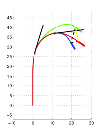
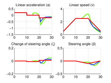
It is crucial that the deformation at $\tau_{2}$ is made first (and the deformation at $\tau_{1}$ only second) so as to leave the velocity vector at $\tau_{1}$ unchanged ($\mathbf{v}^{\prime}(\tau_{1})=\mathbf{v}(\tau_{1})$).

III-D5 Trajectory correction IV: position and orientation correction using three affine deformations

Composing three affine deformations allows achieving both the desired final position and orientation as follows (see Fig. 5)

1. select three (non-inflection) time instants $\tau_{1}$, $\tau_{2}$, and $\tau_{3}$ with $\tau_{1}<\tau_{2}<\tau_{3}$, such that $\mathbf{v}(\tau_{1})$, $\mathbf{v}(\tau_{2})$ and $\mathbf{v}(\tau_{3})$ are pairwise non-collinear. Such three time instants exist since $\mathcal{C}$ is not a straight line;

2. apply a first deformation on $\mathcal{C}$ at $\tau_{3}$ to obtain $\mathcal{C}^{\prime}$, with $\mathcal{C}^{\prime}(T)=\mathcal{C}(T)+\alpha_{3}\mathbf{v}(\tau_{3})$, where $\alpha_{3}$ is a coefficient to be tuned later;

3. following the results of the previous section, one can use the second and third deformations to correct back to the desired position $\mathcal{C}^{\prime\prime\prime}(T)=P_{d}$. Remark that the final orientation of $\mathcal{C}^{\prime\prime\prime}$ depends on $\alpha_{3}$ as shown in Fig. 5. The formula to algebraically compute $\alpha_{3}$ as a function of the desired final orientation can be obtained in a similar way as in section III-D3.

Figure 5: Position and orientation correction using three successive affine deformations. The left and right plots correspond to two different values of $\alpha_{3}$. Remark that the trajectory $\mathcal{C}^{\prime\prime\prime}$ (magenta) ends at the same position ($P_{d}=(20,40)$) in the left and right plots, but that its final orientation differs significantly between the two plots. By varying $\alpha_{3}$, it is thus possible to cover a large range of possible desired final orientations while keeping the desired final position fixed.

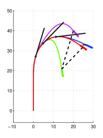
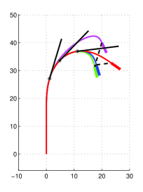
Finally, remark that one can also set the final linear speed to arbitrary values while keeping the final position and orientation unchanged by using the extension technique of section V-D.

IV Affine trajectory correction for a tridimensional underwater vehicle

IV-A Model description

A tridimensional underwater vehicle can be modeled by the following equations [16]

$$\left\{\begin{array}[]{ccc}\dot{x}&=&v\cos\psi\cos\theta\\ \dot{y}&=&v\sin\psi\cos\theta\\ \dot{z}&=&-v\sin\theta\\ \left(\begin{array}[]{c}\dot{\phi}\\ \dot{\theta}\\ \dot{\psi}\end{array}\right)&=&\mathbf{R}(\phi,\theta)\left(\begin{array}[]{c}\omega_{x}\\ \omega_{y}\\ \omega_{z}\end{array}\right)\end{array}\right.,$$ (13)

where $(v,\omega_{x},\omega_{y},\omega_{z})$ are the system commands, $(x,y,z,\phi,\theta,\psi)$ the system variables, and

$$\mathbf{R}(\phi,\theta)=\left(\begin{array}[]{ccc}1&\sin\phi\tan\theta&\cos\phi\tan\theta\\ 0&\cos\phi&-\sin\phi\\ 0&\sin\phi\sec\theta&\cos\phi\sec\theta\end{array}\right).$$

We choose $x$, $y$, and $z$ to be the base variables. The base space is thus of dimension 3. The non-base variables are $\phi$, $\theta$, and $\psi$.

As in the case of planar wheeled robots, the admissible commands $v$ are assumed to be in $\mathscr{D}^{1}$ (allowing possible discontinuities in the linear acceleration). The admissible commands $\omega_{x}$, $\omega_{y}$, and $\omega_{z}$ are assumed to be in $\mathscr{D}^{0}$.

IV-B Admissible base-space trajectories

Following the same line of reasoning as previously, a necessary condition for the admissibility of a base-space trajectory $\mathcal{C}(t)_{t\in[0,T]}=(x(t),y(t),z(t))_{t\in[0,T]}$ is that $x$, $y$ and $z$ belong to $\mathscr{D}^{2}$.

Conversely, assume that $x$, $y$ and $z$ belong to $\mathscr{D}^{2}$. Remark first that, from the system equations (13), the “roll” angle $\phi$ is independent of $(x(t),y(t),z(t))_{t\in[0,T]}$. Next, given an arbitrary roll angle profile $\phi(t)_{t\in[0,T]}\in\mathscr{D}^{1}$, one can safely write the following reverse equations (assuming that the velocity is always strictly positive and that the trajectory stays away from the singularities of the Euler angles [16])

$$\left\{\begin{array}[]{ccc}\psi&=&\mathrm{arctan2}(\dot{y},\dot{x})\\ v&=&\sqrt{\dot{x}^{2}+\dot{y}^{2}+\dot{z}^{2}}\\ \theta&=&\arcsin(\dot{z}/v)\\ \left(\begin{array}[]{c}\omega_{x}\\ \omega_{y}\\ \omega_{z}\end{array}\right)&=&\mathbf{R}(\phi,\theta)^{-1}\left(\begin{array}[]{c}\dot{\phi}\\ \dot{\theta}\\ \dot{\psi}\end{array}\right)\end{array}\right.,$$

In summary, a base-space trajectory is admissible if and only if it is in $\mathscr{D}^{2}$.

IV-C Admissible affine deformations

Consider now an admissible base-space trajectory $\mathcal{C}$ and an affine deformation $\mathcal{F}$ occurring at time $\tau$ that deforms $\mathcal{C}$ in to $\mathcal{C}^{\prime}$. As in section III-C1, one can show that $\mathcal{C}^{\prime}(t)_{t\in(\tau,T]}$ belongs to $\mathscr{D}^{2}$, owing to the smoothness of $\mathcal{F}$.

At the time instant $\tau$, the continuities of $x$, $y$ and $z$ impose that $\mathcal{F}(\mathcal{C}(\tau))=\mathcal{C}(\tau)$. Thus $\mathcal{F}$ can be written in the form

$$\forall P\in\mathbb{A}\quad\mathcal{F}(P)=\mathcal{C}(\tau)+\mathcal{M}(\overrightarrow{\mathcal{C}(\tau)P}).$$ (14)

Next, following again the same reasoning as in section III-C1, the continuities of $v$, $\psi$ and $\theta$ are equivalent to setting $\mathcal{M}(\mathbf{v}(\tau))=\mathbf{v}(\tau)$.

In summary, an affine deformation $\mathcal{F}$ occurring at time $\tau$ is admissible if and only if $\mathcal{M}(\mathbf{v}(\tau))=\mathbf{v}(\tau)$ when $\mathcal{F}$ is written in the form (14). As a consequence, the admissible affine transformations at time $\tau$ form a Lie group of dimension 6.

In practice, we shall compute $\mathcal{M}$ in the basis $\{\mathbf{u}_{\|},\mathbf{w}_{1},\mathbf{w}_{2}\}$ where $\mathbf{w}_{1}$ and $\mathbf{w}_{2}$ are two arbitrary unit vectors forming an orthonormal basis with $\mathbf{u}_{\|}$. In this basis, the condition $\mathcal{M}(\mathbf{v}(\tau))=\mathbf{v}(\tau)$ is equivalent to setting the first column of the matrix that represents $\mathcal{M}$ to $(1,0,0)$. It suffices then to find the six remaining coefficients.

IV-D Trajectory correction

We consider only the correction of the final position, at a given $\tau$. It is possible to achieve more complex corrections as well (correcting the final orientation, avoiding obstacles, etc.) or to optimize the time instant $\tau$: these developments are left to the reader.

Theoretically, three free coefficients are sufficient to reach any final position. As a consequence, we have here more coefficients than needed. We solve this “redundancy” problem by choosing an affine transformation that is the “closest” to the identity matrix, i.e., that affects the least the original trajectory.

As in section III-C2, to correct towards a desired position $P_{d}=(x_{d},y_{d},z_{d})$, one needs to look for a linear application $\mathcal{M}$ such that

$$\mathcal{M}(\overrightarrow{\mathcal{C}(\tau)\mathcal{C}(T)})=\overrightarrow{\mathcal{C}(\tau)P_{d}}.$$ (15)

Let $\mathbf{Q}=[\mathbf{u}_{\|},\mathbf{w}_{1},\mathbf{w}_{2}]$ and let the matrix representing $\mathcal{M}$ in the basis $\{\mathbf{u}_{\|},\mathbf{w}_{1},\mathbf{w}_{2}\}$ be

$$\mathbf{M}=\left(\begin{array}[]{ccc}1&\lambda&\mu\\ 0&1+\nu&\xi\\ 0&\sigma&1+\chi\end{array}\right).$$

Equation (15) implies

$$\mathbf{Q}\mathbf{M}\mathbf{Q}^{-1}\left(\begin{array}[]{c}x(T)-x(\tau)\\ y(T)-y(\tau)\\ z(T)-z(\tau)\end{array}\right)=\left(\begin{array}[]{c}x_{d}-x(\tau)\\ y_{d}-y(\tau)\\ z_{d}-z(\tau)\end{array}\right).$$ (16)

Let next

$$\left(\begin{array}[]{c}x_{1}\\ y_{1}\\ z_{1}\end{array}\right)=\mathbf{Q}^{-1}\left(\begin{array}[]{c}x(T)-x(\tau)\\ y(T)-y(\tau)\\ z(T)-z(\tau)\end{array}\right),$$

$$\left(\begin{array}[]{c}x_{2}\\ y_{2}\\ z_{2}\end{array}\right)=\mathbf{Q}^{-1}\left(\begin{array}[]{c}x_{d}-x(\tau)\\ y_{d}-y(\tau)\\ z_{d}-z(\tau)\end{array}\right).$$

Equation (16) then implies

$$\mathbf{U}\left(\begin{array}[]{c}\lambda\\ \mu\\ \nu\\ \xi\\ \sigma\\ \chi\end{array}\right)=\left(\begin{array}[]{c}x_{2}-x_{1}\\ y_{2}-y_{1}\\ z_{2}-z_{1}\end{array}\right),$$ (17)

where

$$\mathbf{U}=\left(\begin{array}[]{cccccc}y_{1}&z_{1}&0&0&0&0\\ 0&0&y_{1}&z_{1}&0&0\\ 0&0&0&0&y_{1}&z_{1}\end{array}\right).$$

The $(\lambda,\mu,\nu,\xi,\sigma,\chi)$ with minimal norm (i.e. that yields a $\mathcal{M}$ closest to identity according to the Frobenius distance) and that satisfies the under-determined system (17) is given by

$$\mathbf{U}^{+}\left(\begin{array}[]{c}x_{2}-x_{1}\\ y_{2}-y_{1}\\ z_{2}-z_{1}\end{array}\right),$$

where $\mathbf{U}^{+}$ denotes the Moore-Penrose pseudo-inverse of $\mathbf{U}$.

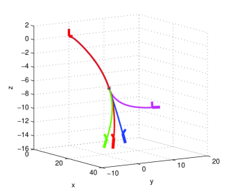
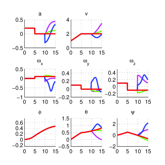
Finally, one needs to choose the “independent” angle $\phi(t)_{t\in[\tau,T]}$. Here our strategy consists of keeping the same $\phi$ as in the original trajectory. Other strategies (e.g. keeping the same absolute roll as in the original trajectory) can also be used. Fig. 6 shows some examples of trajectory corrections.

Figure 6: Examples of trajectory corrections for an underwater vehicle. The original trajectory is in red.

V Further applications

We now use the trajectory correction algorithms just developped as basic tools to tackle more complex tasks. We mostly use the kinematic car (which is a wheeled robot of type (1,1) and class II, see section III-B4) as illustrative example but the following developments can be easily adapted to other nonholonomic systems, provided that affine corrections are available for these systems.

V-A Wheeled robots towing trailers

A kinematic car towing $p$ trailers can be modeled by

$$\left\{\begin{array}[]{ccc}\dot{x}&=&v\cos(\theta_{0})\\ \dot{y}&=&v\sin(\theta_{0})\\ \dot{\theta}_{0}&=&\frac{v\tan(\beta)}{L_{0}}\\ \dot{\beta}&=&\zeta\\ &&\textrm{and for $i=1\dots p$}\\ \dot{\theta}_{i}&=&\frac{v}{L_{i}}\left(\prod_{j=1}^{i-1}{\cos(\theta_{j-1}-\theta_{j})}\right)\sin(\theta_{i-1}-\theta_{i})\end{array}\right.,$$ (18)

where $(v,\zeta)$ are the system commands (respectively the linear velocity of the car and the rate of change of the steering angle) and $(x,y,\beta,\theta_{0},\theta_{1},\dots\theta_{n})$, the system variables (respectively, the $x$ and $y$ coordinates of the car in the laboratory reference frame, the steering angle, the angle of the car with respect to the laboratory reference frame, the angle of the first trailer with respect to the laboratory reference frame, etc.).

The same reasoning as in the case of the simple kinematic car shows that a base-space trajectory $\mathcal{C}=(x,y)$ is admissible only if it belongs to $\mathscr{D}^{2}$ and if $\theta_{0}$ – computed from $\mathcal{C}$ by $\theta_{0}=\mathrm{arctan2}(\dot{y},\dot{x})$ – belongs to $\mathscr{D}^{2}$. Conversely, assume that $\mathcal{C}$ is in $\mathscr{D}^{2}$ and $\theta_{0}$ – computed from $\mathcal{C}$ – is in $\mathscr{D}^{2}$. One can then safely compute $v\in\mathscr{D}^{1}$, $\beta\in\mathscr{D}^{1}$, $\theta_{0}\in\mathscr{D}^{2}$ (by assumption) and $\zeta\in\mathscr{D}^{0}$ as in the case of the simple car. Next, to obtain $\theta_{i}$ (for $i=1\dots n$), it suffices to solve successively the following (ordinary) differential equations

$$\dot{\theta}_{i}=\frac{v}{L_{i}}\left(\prod_{j=1}^{i-1}{\cos(\theta_{j-1}-\theta_{j})}\right)\sin(\theta_{i-1}-\theta_{i})$$

In summary, the set of admissible base-space trajectories of a car towing $p$ trailers is the same as that of a simple car. As a consequence, the admissible affine deformations and the trajectory correction algorithms for a car towing $p$ trailers are also the same as those for a simple car. An example of trajectory correction for a car towing two trailers is given in Fig. 7.

Note that we have no “control” over the configurations of the trailers, contrary to the literature (transformations to chained forms [15, 20], flatness theory [6], etc.). However, consider the (commonly encountered) case when the end of the initially planned trajectory consists of a straight segment, in order to align the trailers with the car. Since affine transformations preserve collinearity, the end of the corrected trajectory will also consist of a straight line, which automatically guarantees the alignment of the trailers with the car.

Note finally that it could be interesting to study affine deformations of the trajectory of the flat output [6], which is, in the present case, the middle of the rear wheels axle of the last trailer (assuming that each trailer is hooked up at the middle of the rear wheels axle of the preceding trailer).

Figure 7: Trajectory correction for a car towing two trailers. One can imagine the following scenario: a trajectory $\mathcal{C}$ (red) is initially planned to park the car with trailers in a given parking slot; following the occupation of that parking slot, a new trajectory $\mathcal{C}^{\prime\prime\prime}$ (magenta) is obtained by deforming the red trajectory using the algorithm of section III-D5 (where the blue and green trajectories correspond respectively to $\mathcal{C}^{\prime}$ and $\mathcal{C}^{\prime\prime}$). The new trajectory allows the car to be parked in a neighboring slot, with the same final orientation. Note that the collinearity-preserving property of affine transformations automatically guarantees the straightness of the final segments of the blue, green and magenta trajectories, which in turn implies the alignment of the trailers with the car.

V-B Obstacle avoidance

In the trajectory correction algorithms previously developped, one can in fact replace the final time $T$ by any time instant $t>\tau$. This allows implementing interactive obstacle avoidance algorithms as follows

1. determine a time instant $t_{\mathrm{obs}}$ when the initially planned trajectory would collide with the obstacle;

2. select a new, non colliding, intermediate position $(x_{\mathrm{inter}},y_{\mathrm{inter}})$ to which one could make a correction;

3. make the correction of $(x(t_{\mathrm{obs}}),y(t_{\mathrm{obs}}))$ towards $(x_{\mathrm{inter}},y_{\mathrm{inter}})$, using $\tau$(s) $<t_{\mathrm{obs}}$;

4. re-correct the final position towards the initially planned final position, using $\tau$(s) $\geq t_{\mathrm{obs}}$.

Figure 8: An example of obstacle avoidance for the unicycle. The original trajectory $(x,y)$ (red) was planned knowing the position of the black obstacles. During the execution, an unforeseen obstacle (cyan) appears on the original path. A new trajectory $(x_{1},y_{1})$ (blue) is obtained by deforming the original trajectory. The blue star indicates the position $(x(\tau_{1}),y(\tau_{1}))$ where the deformation occurs, and the black plain line joins $(x(t_{\mathrm{obs}}),y(t_{\mathrm{obs}}))$ to $(x_{\mathrm{inter}},y_{\mathrm{inter}})$. Next, in order to get back to the original target, an other trajectory (green) is obtained by deforming the blue one. The green star indicates the position $(x_{1}(\tau_{2}),y_{1}(\tau_{2}))$ where the deformation occurs, and the black dashed line joins $(x_{1}(T),y_{1}(T))$ to $(x(T),y(T))$.

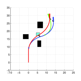
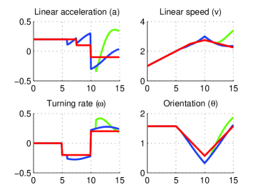
This algorithm can be run iteratively to avoid all obstacles.

One can also prescribe a specific position/orientation of the trajectory at a given time instant $t_{\mathrm{door}}$ (this is desirable for instance when two large obstacles are close to each other, leaving between them a small doorway through which the robot could go), as follows

1. make the correction of $(x(t_{\mathrm{door}}),y(t_{\mathrm{door}}))$ towards the specified intermediate position;

2. make the correction of $\theta(t_{\mathrm{door}})$ towards the specified intermediate orientation;

3. re-correct the final position towards the initially planned final position, using $\tau$(s) $>t_{\mathrm{door}}$.

V-C Feedback control

So far, we have been focusing on perturbations affecting the state of the target (position and/or orientation) or the environment (unexpected appearance of obstacles). Here we show, through a simplified feedback control algorithm, how affine corrections can also be used to deal with perturbations affecting the robot’s own state.

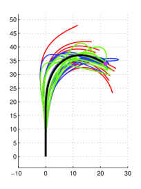
Consider again the example of the kinematic car. Assume that a trajectory has been initially planned (black trajectory in Fig. 9A), in terms of the time series of the control inputs $(a_{\mathrm{plan}}(t)_{t\in[0,T]},\zeta_{\mathrm{plan}}(t)_{t\in[0,T]})$. Assume now that these control imputs are corrupted by random perturbations

$$\forall t\in[0,T]\quad\left\{\begin{array}[]{ccc}a(t)&=&a_{\mathrm{plan}}(t)+\xi_{1}(t)\\ \zeta(t)&=&\zeta_{\mathrm{plan}}(t)+\xi_{2}(t)\end{array}\right.,$$

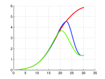
where $\xi_{1}$ and $\xi_{2}$ two piecewise constant random functions. The red trajectories in Fig. 9A represent several trajectories of the car corresponding to different realizations of the pertubations $\xi_{1}$ and $\xi_{2}$. One can notice that the perturbations make the final positions of the red trajectories deviate randomly from the target (denoted by the magenta dot). This can also be noted from the variability profile (red curve in Fig. 9B), which is nonzero at the end of the movement.

A

B

Figure 9: Feedback control using affine corrections. A: uncorrected sample trajectories (red), corrected using at most one correction (blue) or at most five corrections (green). The initially planned trajectory is in black. B: variability profiles computed across 2000 realizations of the random perturbations $\xi_{1}$ and $\xi_{2}$.

We propose the following feedback control algorithm inspired from [21, 18]. The algorithm maintains at every step two time series $(a_{\mathrm{cur}}(t)_{t\in[0,T]},\zeta_{\mathrm{cur}}(t)_{t\in[0,T]})$ termed “currently planned control inputs”. These time series are initialized at the values of $(a_{\mathrm{plan}}(t)_{t\in[0,T]},\zeta_{\mathrm{plan}}(t)_{t\in[0,T]})$. The movement time $T$ is divided in $S+1$ equal parts. At each time instant $t_{i}=iT/(S+1)$, $i=1\dots S$, the robot is given the possibility to make a correction as follows

1. compute the final position of the robot, had the control inputs $(a_{\mathrm{cur}}(t)_{t\in[t_{i},T]},\zeta_{\mathrm{cur}}(t)_{t\in[t_{i},T]})$ been applied starting at the current state $\bar{\mathcal{C}}(t_{i})$ and until the end of the movement. Denote this final simulated position $(x_{\mathrm{sim}},y_{\mathrm{sim}})$;

2. compute appropriate trajectory deformations with $\tau(s)>t_{i}$ to correct the final position from $(x_{\mathrm{sim}},y_{\mathrm{sim}})$ towards $(x_{\mathrm{target}},y_{\mathrm{target}})$. This gives rise to new time series of control inputs, denoted $(a_{\mathrm{new}}(t)_{t\in[t_{i},T]},\zeta_{\mathrm{new}}(t)_{t\in[t_{i},T]})$;

3. if the new control inputs are acceptable (i.e. do not imply too large accelerations or too sharp turns), set $a_{\mathrm{cur}}(t)_{t\in[t_{i},T]}\leftarrow a_{\mathrm{new}}(t)_{t\in[t_{i},T]}$ and $\zeta_{\mathrm{cur}}(t)_{t\in[t_{i},T]}\leftarrow\zeta_{\mathrm{new}}(t)_{t\in[t_{i},T]}$. Otherwise, keep the current values of $a_{\mathrm{cur}}$ and $\zeta_{\mathrm{cur}}$.

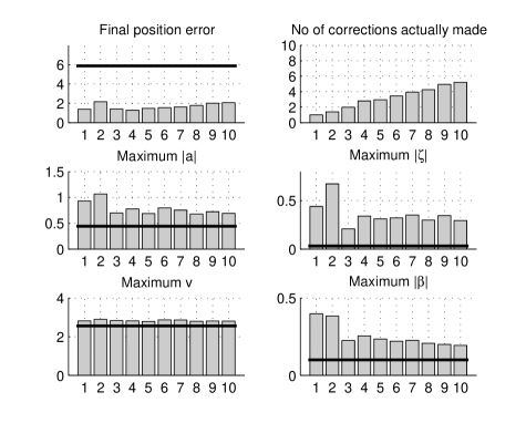
Figure 9A shows the results of the feedback control algorithm for $S=1$ (blue curves) and $S=5$ (green curve). Note that the blue and green curves are driven by the same realizations of the perturbations as the red curves (uncorrected trajectories). However, the blue and green curves end up much closer to the target position. Figure 9B confirms this observation: the final variabilities of the corrected trajectories (blue and green profiles) at $T$ are much lower ($\sim$1.3m) than that of the uncorrected trajectories ($\sim$6m).

One could ask: why make multiple corrections (green) while making one unique correction (blue) yields approximately the same final average error? Figure 10 shows that $S=1$ is associated with larger values of $a$, $\zeta$ and $\beta$ than $S=5$. This is because when the robot is allowed to make multiple corrections, the changes to $a$ and $\zeta$ are distributed instead of being concentrated in one single large correction near the end of the trajectory. Figure 9B confirms this observation: the green variability profile ($S=5$) starts decreasing before the blue variability profile ($S=1$). Note however that choosing $S>5$ does not improve the algorithm.

Figure 10: Statistics of the feedback control algorithm across 2000 realizations of the random perturbations $\xi_{1}$ and $\xi_{2}$. The X-axis represents the maximum number of corrections allowed $S$. The horizontal lines report the values corresponding to the uncorrected trajectories ($S=0$).

Finally, note that this algorithm is not a trajectory-tracking algorithm but rather a simplified implementation of “optimal feedback control” [21, 18].

V-D Gap filling for sampling-based kinodynamic planners

Gap-reduction techniques are a core component of any sampling-based kinodynamic planner [4]. As an example, consider the approach proposed in [14], which consists of growing two rapidly-exploring random tree (RRT) rooted respectively at the initial state and at the target state – a solution trajectory is obtained when these two trees intersect. When nonholonomic constraints are present, exact intersections of the trees occur with probability zero, such that one usually assumes intersection when the trees are within a nonzero distance of each other, yielding thereby a gap in the solution trajectory. As the performance of the planner critically depends on the permitted gap size (the larger the permitted gap size, the quicker the growing trees find an “intersection”, but also the more difficult filling the gaps), efficient gap-reduction techniques have been shown to dramatically improve the performance of the planner [4].

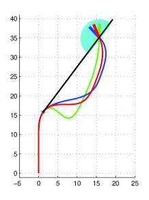
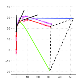
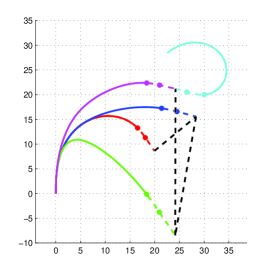
We now show how affine corrections can be used to fill trajectory gaps. Consider two trajectories $\mathcal{C}_{1}(t)_{t\in[0,T_{1}]}$ and $\mathcal{C}_{2}(t)_{t\in[0,T_{2}]}$ of a kinematic car (respectively in red and cyan in Fig. 11) separated by a gap. We first “prepare” the two trajectories as follows

1. grow a first stub with time duration $\Delta_{a}$ at the end of $\mathcal{C}_{1}$. Using the time interval $[T_{1},T_{1}+\Delta_{a}]$, bring the steering angle $\beta_{1}$ to 0 by “counter-steering” (i.e. turning the steering wheel back to the straight-ahead position);

2. grow a second stub with time duration $\Delta_{b}$ at the end of the extended $\mathcal{C}_{1}(t)$. During this time interval, the steering angle $\beta_{1}$ is kept to 0, resulting in a straight segment. One can easily verify that the (doubly) extended trajectory $\mathcal{C}_{1}(t)_{t\in[0,T_{1}+\Delta_{a}+\Delta_{b}]}$ is admissible. The two stubs are shown by dashed red lines in Fig. 11;

3. similarly, grow two other stubs at the beginning of $\mathcal{C}_{2}$ (shown by dashed cyan lines in Fig. 11).

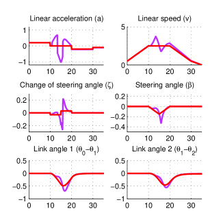
After this “preparation”, we have two trajectories which respectively ends and begins by straight segments. The lengths of the added stubs depend on the $\Delta$s and can be made relatively short if the $\beta$s are small and large braking and counter-steering rates are permitted. We can now use the position and orientation algorithms given in the previous sections to bring the end of the extended $\mathcal{C}_{1}$ towards the beginning of the extended $\mathcal{C}_{2}$. Fig. 11 shows an example of such correction using three succesive affine deformations (cf. section III-D5). The admissibility conditions are verified by observing that

• since affine transformations preserve collinearity, the corrected extended trajectory $\mathcal{C}^{\prime\prime\prime}_{1}$ (magenta) also ends by a straight segment. When this straight segment connects with the straight segment at the beginning of the extended $\mathcal{C}_{2}$, the continuity of $\beta$ is guaranteed;

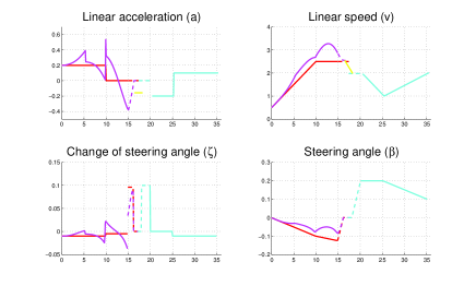
• regarding the continuity of $v$, one can use the straight parts around the connection point to modulate the speed profile to make it continuous without altering the geometric path: see the yellow lines in the plots of $a$ and $v$ in Fig. 11.

Figure 11: Filling trajectory gaps. Top plot: geometric paths. The original trajectories to be connected are showned in plain red line ($\mathcal{C}_{1}$) and plain cyan line ($\mathcal{C}_{2}$). These trajectories are first “prepared” by growing stubs at their extremities (red and cyan dashed lines). The extended $\mathcal{C}_{1}$ is then corrected into $\mathcal{C}^{\prime\prime\prime}_{1}$ (magenta) by three successive affine deformations (the blue and green lines represent the intermediate trajectories $\mathcal{C}^{\prime}_{1}$ and $\mathcal{C}^{\prime\prime}_{1}$ ). Note that $\mathcal{C}^{\prime\prime\prime}_{1}$ smoothly connects with $\mathcal{C}_{2}$. Bottom plot: profiles of the other variables. The yellow lines in the plots of $a$ and $v$ show the modifications that make $v$ continuous without changing the geometric paths.

VI Discussion

As stated at the beginning of section III, one can apply the following general scheme to study affine trajectory corrections for nonholonomic systems

1. check the conditions for a base-space trajectory to be admissible. Often (but not always), a base-space trajectory is admissible if it – and some functions computed from it – belong to certain classes $\mathscr{D}^{i}$;

2. based on the admissibility conditions of trajectories, particularly at the time instant when the deformation occurs, characterize the set of admissible affine deformations. Often (but not always), the admissible affine deformations at a given time instant form a Lie group of dimension $n+n^{2}-m$ where $n$ is the number of base variables and $m$ the number of continuity conditions;

3. finally, play with $\tau$ and the $n+n^{2}-m$ “extra degrees of freedom” to achieve the desired correction. If there are more “extra degrees of freedom” than needed, one can “optimize” by choosing the affine transformations that are the closest to identity.

This general scheme suggests in turn the classes of systems that can or cannot be tackled by the proposed method. For instance, an underwater vehicle whose changes in turning rate ($\rho_{x}=\dot{\omega}_{x}$, $\rho_{y}=\dot{\omega}_{y}$, $\rho_{z}=\dot{\omega}_{z}$) are required to be continuous could probably be treated by the method (since in this case $n+n^{2}-m=3$). The development of the theory to deal with other classes of nonholonomic systems are also the subject of ongoing efforts.

Holonomic systems, such as the end-point of a robotic manipulator, are not subject, by nature, to the differential constraints with which the current manuscript is concerned. However, it is sometimes desirable for efficiency reasons to artificially enforce some differential constraints, such as the continuity of the velocity vector. For instance, if a planned path is not $\mathscr{C}^{1}$ at some points, the robot must stop-and-start at these points [9], which clearly is an undesired behavior. In this perspective, the regularity-preserving deformation algorithms developped here can also be useful for holonomic trajectory planning.

As just remarked, this manuscript is mostly concerned with the differential constraints that stem from the nonholonomic nature of the considered systems. In practice, other constraints, such as upper limits on the absolute acceleration or on the trajectory curvature, could further restrict the set of admissible affine deformations. This can be treated by observing that the changes in acceleration or curvature from the original trajectory can be computed from the affine transformation at hand (see also [1]). The integration of such constraints into the current framework represents an important task (see e.g. [8]).

Another promising direction of research may consist of combining the approach presented here with existing approaches for trajectory planning and deformation. We have mentioned earlier possible interactions with flatness theory. A complementary use of affine-based and perturbation-based deformations [12] may also lead to more efficient algorithms. For instance, affine corrections perform badly when the original trajectory is close to a straight line. Using the results in [12], it should be possible to slightly perturb the original trajectory to generate local curved portions, which subsequently allow applying affine deformations with greater effectiveness.

As mentioned in the Introduction, one advantage of the method presented in this manuscript is that it requires no re-integration of the trajectory. On the other hand, differentiations of the trajectory must be performed in order to recover the commands (see “Important remark” in section III-B6). Note however that, if multiple deformations are made, the differentiations need to be performed only once, after all the deformations have been applied.

The group property of affine transformations can also be used to further accelerate the computations (as in [19] with Euclidean transformations). Assume for instance that two affine transformations $\mathcal{F}_{1}$ and $\mathcal{F}_{2}$ are applied at time instants $\tau_{1}$ and $\tau_{2}$, with $\tau_{1}<\tau_{2}$. Then one can apply $\mathcal{F}_{1}$ to $\mathcal{C}(t)_{t\in[\tau_{1},\tau_{2}]}$ and next $\mathcal{F}_{2}\circ\mathcal{F}_{1}$, which is also an affine transformation, to $\mathcal{C}(t)_{t\in(\tau_{2},T]}$.

Another advantage, also mentioned in the Introduction, is that the method presented here can be executed in one step, while other methods require iterative deformations of the trajectory [12] or gradient descent to find the appropriate deformation coefficients [4, 19]. This may result in significant performance gains, in particular, in real-time applications or in highly compute-intensive tasks such as the building of probabilistic roadmaps [14].

Finally, the method is exact: for example, a desired position can be reached exactly, and not only approached iteratively “as close as we want”. This may have important consequences. For example, in the initial trajectory planning, one would no longer need to spend time finding a trajectory that ends very close to the target. Instead, one can plan a trajectory that ends roughly somewhere near the target, and then make an affine deformation towards the exact target position.

A last word on the biological implications of the ideas presented here. One source of inspiration for the present work was indeed the recent studies of affine invariance in human perception and movements (see e.g. [1] and references therein). Conversely, one could ask (and experimentally test) whether humans use algorithms similar to those described here to correct their hand or locomotor trajectories.

Acknowledgments

The author is deeply grateful to Prof. Daniel Bennequin, Prof. Yoshihiko Nakamura, and Dr. Oussama Kanoun for their highly valuable suggestions and comments. This research was funded by an University of Tokyo grant and by a JSPS postdoctoral fellowship.

References

- Bennequin et al. [2009] D. Bennequin, R. Fuchs, A. Berthoz, and T. Flash. Movement timing and invariance arise from several geometries. PLoS Comput Biol, 5(7):e1000426, Jul 2009. doi: 10.1371/journal.pcbi.1000426.
- Boissonnat et al. [1994] J.D. Boissonnat, A. Cerezo, and J. Leblond. A note on shortest paths in the plane subject to a constraint on the derivative of the curvature. Rapports de recherche-INRIA, 1994. ISSN 0249-6399.
- Campion et al. [1996] G. Campion, G. Bastin, and B. D’Andrea-Novel. Structural properties and classification of kinematic and dynamic models of wheeled mobile robots. IEEE Transactions on Robotics, 12(1):47–62, 1996. doi: 10.1109/70.481750.
- Cheng et al. [2008] P. Cheng, E. Frazzoli, and S. LaValle. Improving the performance of sampling-based motion planning with symmetry-based gap reduction. IEEE Transactions on Robotics, 24(2):488–494, 2008. ISSN 1552-3098.
- Filippov [1988] A. Filippov. Differential equations with discontinuous righthand sides. Springer, 1988. ISBN 902772699X.
- Fliess et al. [1995] M. Fliess, J. Lévine, P. Martin, and P. Rouchon. Flatness and defect of non-linear systems: introductory theory and examples. International journal of control, 61(6):1327–1361, 1995. ISSN 0020-7179.
- Fraichard and Scheuer [2004] T. Fraichard and A. Scheuer. From Reeds and Shepp’s to continuous-curvature paths. IEEE Transactions on Robotics, 20(6):1025–1035, 2004. doi: 10.1109/TRO.2004.833789.
- Hillion and Lamiraux [2007] M. Hillion and F. Lamiraux. Taking into account velocity and acceleration bounds in nonholonomic trajectory deformation. In Robotics and Automation, 2007 IEEE International Conference on, pages 3080–3085. IEEE, 2007. ISBN 1424406013.
- Kanehiro et al. [2008] F. Kanehiro, W. Suleiman, F. Lamiraux, E. Yoshida, and J.P. Laumond. Integrating dynamics into motion planning for humanoid robots. In Intelligent Robots and Systems, 2008. IROS 2008. IEEE/RSJ International Conference on, pages 660–667. IEEE, 2008.
- Kelly and Nagy [2003] A. Kelly and B. Nagy. Reactive nonholonomic trajectory generation via parametric optimal control. The International Journal of Robotics Research, 22(7-8):583, 2003. ISSN 0278-3649.
- Khatib et al. [1997] M. Khatib, H. Jaouni, R. Chatila, and J.P. Laumond. Dynamic path modification for car-like nonholonomic mobile robots. In IEEE International Conference on Robotics and Automation, 1997. ISBN 0780336127.
- Lamiraux et al. [2004] F. Lamiraux, D. Bonnafous, and O. Lefebvre. Reactive path deformation for nonholonomic mobile robots. IEEE Transactions on Robotics, 20(6):967–977, 2004. doi: .829459.
- Laumond [1998] J.-P. Laumond. Robot Motion Planning and Control. Springer-Verlag, New York, 1998.
- LaValle and Kuffner [2001] S.M. LaValle and J.J. Kuffner. Randomized kinodynamic planning. The International Journal of Robotics Research, 20(5):378, 2001. ISSN 0278-3649.
- Murray and Sastry [1993] R. M. Murray and S. S. Sastry. Nonholonomic motion planning: steering using sinusoids. IEEE Transactions on Automatic Control, 38(5):700–716, 1993. doi: 10.1109/9.277235.
- Nakamura and Savant [1992] Y. Nakamura and S. Savant. Nonlinear tracking control of autonomous underwater vehicles. In IEEE International Conference on Robotics and Automation, 1992. doi: 10.1109/ROBOT.1992.220005.
- Pham [2011] Q.-C. Pham. Fast trajectory correction for nonholonomic mobile robots using affine transformations. In Robotics: Science and Systems, 2011.
- Pham and Hicheur [2009] Q.-C. Pham and H. Hicheur. On the open-loop and feedback processes that underlie the formation of trajectories during visual and nonvisual locomotion in humans. J Neurophysiol, 102(5):2800–15, November 2009. ISSN 1522-1598.
- Seiler et al. [2010] K. Seiler, S. Singh, and H. Durrant-Whyte. Using Lie group symmetries for fast corrective motion planning. In Algorithmic Foundations of Robotics IX, 2010.
- Sordalen and Egeland [1995] O. J. Sordalen and O. Egeland. Exponential stabilization of nonholonomic chained systems. IEEE Transactions on Automatic Control, 40(1):35–49, 1995. doi: 10.1109/9.362901.
- Todorov and Jordan [2002] E. Todorov and M.I. Jordan. Optimal feedback control as a theory of motor coordination. Nat Neurosci, 5(11):1226–35, November 2002. ISSN 1097-6256.