Exact infinite-time statistics of the Loschmidt echo for a quantum quench

Abstract

The equilibration dynamics of a closed quantum system is encoded in the long-time distribution function of generic observables. In this paper we consider the Loschmidt echo generalized to finite temperature, and show that we can obtain an exact expression for its long-time distribution for a closed system described by a quantum XY chain following a sudden quench. In the thermodynamic limit the logarithm of the Loschmidt echo becomes normally distributed, whereas for small quenches in the opposite, quasi-critical regime, the distribution function acquires a universal double-peaked form indicating poor equilibration. These findings, obtained by a central limit theorem-type result, extend to completely general models in the small-quench regime.

Introduction

Imagine an isolated quantum system, say the laboratory, prepared in a state $\rho_{0}$. According to the laws of quantum mechanics, the state will evolve unitarily into $\rho\left(t\right)$. The average result of a measurement of an observable $O$ will be the time average $\overline{\langle O\left(t\right)\rangle}:=T^{-1}\int_{0}^{T}\langle O\left(t\right)\rangle dt$, where $T$ is the measurement time. Since $T$ is much larger than the microscopic time scales of the system it is often set to infinity for mathematical clarity. Now, the postulates of statistical mechanics assert that the time-averaged expectation value is indistinguishable from that obtained using the statistical microcanonical ensemble. Although this postulate is confirmed by a number of numerical simulations (see e.g. Rigol et al. (2008)), to date no explanation exists for why this is so. In other words, the mechanisms of thermalization in quantum systems are unknown (though there exist possible approaches such as the eigenstate thermalization hypothesis Deutsch (1991); *srednicki94 or normal typicality von Neumann (1929); *goldstein2009; *tasaki2010).

In such a context it is important to have exact results, at least for some particular cases, which can serve to guide our intuition. Ideally one is interested in the full, long-time statistics of a generic observable $\langle O\left(t\right)\rangle$. This article provides a result in this direction. Namely, concentrating on the Loschmidt echo, we will obtain its exact, long-time distribution function and investigate the effects that proximity to critical points has on the equilibration dynamics. In the thermodynamic limit, also called the off-critical regime, i.e. when the system size is much larger than all length scales of the system, we will see that a central limit theorem result applies leading to universal Gaussian equilibration. In the opposite regime of quasi-criticality, where the correlation length is equal to or larger than the system size, we will again find universal behavior, although one in which fluctuations are large and thermalization does not occur.

The scenario we consider here is that of a quantum quench, generalized to the mixed case. A closed system is initialized in the state $\rho_{0}$ commuting with the Hamiltonian $H_{0}$. The system is then instantaneously quenched and left to evolve according to Hamiltonian $H_{1}$. This is an important generalization, since in principle there is no reason why the “initial” state of the system should be pure. In particular, for its experimental relevance we will use Gibbs initial states $\rho_{0}\sim e^{-\beta H_{0}}$. Such a situation is in fact often realized in the laboratory by first thermalizing the system by putting it in contact with an external reservoir and then detaching the reservoir.

The quantity we consider is the Loschmidt echo (LE), which generalized to the mixed case is given by

$$\mathcal{L}\left(t\right)=F\!\left(\rho\left(t\right),\rho_{0}\right),\,\,F\!\left(\rho,\sigma\right)=\left(\mathrm{tr}\sqrt{\rho^{1/2}\sigma\rho^{1/2}}\right)^{2}.$$

Here $F$ is the Uhlmann fidelity Uhlmann (1976) which characterizes the degree of distinguishability between two mixed states. Note that if either (or both) of $\rho$ and $\sigma$ is pure, the Uhlmann fidelity simplifies to $F\!\left(\rho,\sigma\right)=\mathrm{tr}\left(\rho\sigma\right)$.

The quantum XY chain

The model we investigate here is the quantum XY chain in a transverse magnetic field,

$$H=-\sum_{i=1}^{L}\frac{(1+\gamma)}{2}\sigma_{i}^{x}\sigma_{i+1}^{x}+\frac{(1-\gamma)}{2}\sigma_{i}^{y}\sigma_{i+1}^{y}+h\sigma_{i}^{z}.$$ (1)

A Jordan-Wigner transformation brings Eq. (1) to a quadratic form in Fermi operators $c_{i}$, and hence can be exactly diagonalized. At zero temperature the model (1) displays two kinds of quantum phase transition lines in the $\left(h,\gamma\right)$ plane. For $h=\pm 1$ and $\gamma\neq 0$ the model is in the Ising universality class described by a $c=1/2$ conformal field theory (CFT). Instead, in the segment $\gamma=0$, $\left|h\right|\leq 1$ the underlying CFT has central charge $c=1$. To specify completely the problem we must fix boundary conditions (BC’s). As is customary Barouch et al. (1970), to avoid unnecessary complications we will fix BC’s on the fermions not (a). Diagonalization brings Eq. (1) to free Fermion form: $H=\sum_{k}2\Lambda_{k}\eta_{k}^{\dagger}\eta_{k}$. Our choice of BC’s fixes quasimomenta to be quantized according to $k=\left(2n+1\right)\pi/L$, $n=-L/2,\ldots,L/2-1$, whereas the single-particle dispersion is $\Lambda_{k}=\sqrt{\left(\cos k+h\right)^{2}+\gamma^{2}\sin^{2}k}$.

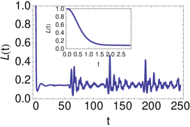
Figure 1: Typical behavior of $\mathcal{L}(t)$. The inset shows Gaussian behavior for short times, as happens for the pure case Campos Venuti and Zanardi (2010a). Here $L=100$, $\beta=6$, $h_{0,1}=1$, $\gamma_{0}=0.5,\,\gamma_{1}=0.8$.

The Loschmidt echo has been shown for the XY chain to be Zanardi et al. (2007a) $\mathcal{L}(t)=\prod_{k>0}f_{k}\left(\Lambda_{k}^{1}t\right)$, with

$$f_{k}\left(\Lambda_{k}^{1}t\right)=\left[\frac{1+\sqrt{c_{k}^{2}-\left(c_{k}^{2}-1\right)\alpha_{k}\sin^{2}(\Lambda_{k}^{1}t)}}{1+c_{k}}\right]^{2}$$ (2)

where $c_{k}=\cosh\left(\beta\Lambda_{k}^{0}\right)$, $\alpha_{k}=\sin^{2}(\Delta\theta_{k})$ , $\Delta\theta_{k}=\theta_{k}^{1}-\theta_{k}^{0}$ and $\theta_{k}=\arctan\left[\gamma\sin\left(k\right)/\left(h+\cos\left(k\right)\right)\right]$. From its explicit form we can read off a number of important points which we will use extensively in the following: i) the time-dependence is governed by $L/2$ frequencies $\Lambda_{k}^{1}$, ii) the LE is a product of an extensive number of terms, and in particular iii) the LE is a product of $L/2$ functions over the $L/2$ allowed values of $k$. The dependence on $k$ is analytic everywhere except for the critical points ($\gamma=0$ and $\left|h\right|\leq 1$ or $\left|h\right|=1$ and $\gamma\neq 0$). No singularity other than those expected at criticality emerges.

Typical behavior of $\mathcal{L}(t)$ is depicted in Fig. 1. The LE quickly drops from unity at $t=0$ and then oscillates about its average value, with almost periodic revivals Häppölä et al. (2010).

Following the spirit of Refs Campos Venuti and Zanardi (2010a, b), we are interested in the distribution function of the LE seen as a random variable over infinite time equipped with the uniform measure. The probability density of the LE can be written as $P_{\mathcal{L}}\left(x\right):=\overline{\delta\left(\mathcal{L}\left(t\right)-x\right)}$, where the bar denotes the time average (i.e. $\overline{f}=\lim_{T\to\infty}T^{-1}\int_{0}^{T}f\left(t\right)dt$). Saying that the LE spends most of the time close to a certain value corresponds to a concentration result for $P_{\mathcal{L}}\left(x\right)$.

The moments of the LE can be computed using the methods developed in Campos Venuti and Zanardi (2010a). Here one has the additional complication given by the presence of the square-root in Eq. (2), which must first be expanded into an infinite series. The result for the first moment is $\overline{\mathcal{L}}=\prod_{k>0}f_{k}^{1}$, with $f_{k}^{1}=1-\left(1-c_{k}^{-1}\right)\frac{\alpha_{k}}{2}+\frac{2c_{k}}{\left(1+c_{k}\right)^{2}}\left[\frac{2}{\pi}E\left(b_{k}\right)+b_{k}/4-1\right]$. Here, $b_{k}=\left(1-c_{k}^{-2}\right)\sin^{2}\left(\Delta\theta_{k}\right)$ and $E$ is the complete elliptic integral of the second kind. Expanding $f_{k}^{1}$ in the small quench regime, that is up to second order in $\Delta\theta_{k}$, one is able to relate the dynamical quantity $\overline{\mathcal{L}}$ to a static quantity. Specifically, one obtains $\overline{\mathcal{L}}\simeq F\left(\rho_{0},\rho_{1}\right)^{2}$, where $\rho_{0,1}$ are Gibbs states with Hamiltonians $H_{0,1}$. This result extends the pure state result $\overline{\mathcal{L}}=\mathrm{tr}\left(\overline{\rho}^{2}\right)\simeq\left|\langle\psi_{0}|\psi_{1}\rangle\right|^{4}$ which can be recovered sending $\beta\to\infty$ Rossini et al. (2007a); *rossini07.

The distribution function for the LE in the Ising model (i.e. $\gamma=1$) at zero temperature was considered in Campos Venuti and Zanardi (2010a). Through numerical simulations it was argued that, in the off-critical regime, two different behaviors were observed. The distribution of the LE was seen as similar to an exponential one, ($P_{\mathcal{L}}\left(x\right)\simeq\vartheta\left(x\right)e^{-x/\overline{\mathcal{L}}}/\overline{\mathcal{L}}$) or to a bell-shaped Gaussian-looking one. In the next section we will unify both of these conjectured results.

Off-critical regime and Gaussian equilibration

The form of the LE suggests that the LE should be thought of as a product of variables. Let us then consider the new variable $Z=\ln\mathcal{L}$. We will show that, under a very mild hypothesis, the variable $Z$ satisfies the standard central limit theorem (CLT). In particular, in the off-critical regime, as $L\to\infty$, the rescaled variable $Y=\left(Z-\overline{Z}\right)/\sqrt{L}$ will tend in distribution to a Gaussian with zero mean and well-defined variance. To this aim we will show that all the cumulants of $Z$ scale extensively, so that for the rescaled variable $Y$ we will get $\kappa_{n}\left(Y\right)\propto L^{1-n/2}$ for $n\geq 2$ while $\kappa_{1}\left(Y\right)=0$ by construction. Hence only the first two cumulants of $Y$ survive in the $L\to\infty$ limit, thus showing Gaussianity of $Y$. In turn, Gaussianity of $Y$ implies that the LE is approximately Log-Normally distributed. This explains the behavior observed in Campos Venuti and Zanardi (2010a), as a Log-Normal has regimes where it looks approximately exponential or Gaussian.

In order to prove our assertion we need the (logarithm of the) moment generating function of $Z$, $M^{Z}\left(\lambda\right):=\overline{e^{\lambda Z}}=\overline{\mathcal{L}^{\lambda}}$. At this point we make the reasonable assumptions that the $L/2$ frequencies $\Lambda_{k}^{1}$ are rationally independent (that is, linearly independent over the field of rational numbers). Thanks to rational independence (RI) we can use the theorem of averages (see e.g. V.I.Arnold (1989) on page 286) to compute the time-average of $\mathcal{L}^{\lambda}$ as a phase space average over an $L/2$-dimensional torus not (b). Our numerical simulations show that a possible rational dependence is very mild and it would be quite unlucky to produce enough correlations to invalidate the CLT. With RI, we obtain

$$M^{Z}\left(\lambda\right)=\prod_{k>0}g_{k}\left(\lambda\right),\,\,g_{k}\left(\lambda\right)=\frac{1}{2\pi}\int_{0}^{2\pi}\left[f_{k}\left(\vartheta\right)\right]^{\lambda}d\vartheta.$$

Hence $M^{Z}\left(\lambda\right)=\exp\sum_{k>0}\ln g_{k}\left(\lambda\right)$. The last steps of the proof come from the fact that $\ln g_{k}\left(\lambda\right)$ as a function of $k$ is Riemann integrable, with a finite integral, provided we are away from critical points. Moreover, in the same region of parameters, $\ln g_{k}\left(\lambda\right)$ (and so its integral over $k$) is analytic in $\lambda$. Specifically, for large $L$, we obtain, $\ln\left[M^{Z}\left(\lambda\right)\right]\simeq LG\left(\lambda\right)$, with $G\left(\lambda\right)=\int_{0}^{\pi}\ln g_{k}\left(\lambda\right)dk/\left(2\pi\right)$ analytic in $\lambda$. Differentiating with respect to $\lambda$ we obtain that all the cumulants of $Z$ are extensive, which completes the proof. $\square$

In particular, one has the CLT anywhere away from the critical points: no other source of singularity emerges other than those expected at criticality.

Let us now pause for a moment and discuss how the CLT could be violated. One possibility is that the variance of $Z$ may grow with $L$ more than extensively, i.e. $\kappa_{2}\left(Z\right)\propto L^{Q}$, with $Q>1$. This would imply that the variance of the rescaled variable would diverge as $L\to\infty$, thus breaking the CLT. It can be shown that $\kappa_{2}\left(Z\right)=\sum_{k>0}\kappa_{2}\left(k\right)$ with $\kappa_{2}\left(k\right)=m_{2}\left(k\right)-\left[m_{1}\left(k\right)\right]^{2}$, and $m_{n}\left(k\right)=\frac{1}{2\pi}\int_{0}^{2\pi}\left[\ln\left(f_{k}\left(\vartheta\right)\right)\right]^{n}d\vartheta$ with $n=1,2$. By direct inspection of the integrals it turns out that $\kappa_{2}\left(k\right)$ is a bounded function in the entire parameter range. Hence $\kappa_{2}\left(Z\right)\leq\mathrm{const.}\times L$ also at critical points.

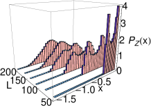
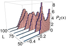
Figure 2: $P_{Z}$ close to the Ising (left) and anisotropy transition (right). As $L$ grows we enter the off-critical regime and $P_{Z}$ becomes Gaussian. Close to the quasi-critical regime (small $L$) the distribution becomes a broad, generally double-peaked function. For the anisotropy transition, one can have $L$ for which the highest amplitudes are nearly equal (see text). This results in a collapse from two peaks to one. Parameters are $\beta=40$ and (left) $h_{0}=0.98,\,h_{1}=1.02,\gamma_{0,1}=1.0$ and $L=50$ to $200$ in steps of $30$, (right) $h_{0,1}=0.5,\,\gamma_{0}=0.01,\gamma_{1}=-0.01$ and $L=50$ to $100$ in steps of $10$. Another way to enter the off-critical regime is to increase the temperature. Similar plots are obtained replacing $L$ with the temperature $T$.

Quasi-critical regime and universal critical equilibration

In Ref. Campos Venuti and Zanardi (2010b) it was argued that for a small quench close to a critical point, no observable (except for trivial constants of motion) thermalizes. Here we will show that this result generalizes to the mixed case considered here. Moreover, as we will see, some universal features of the underlying critical theory show up in the long-time distribution function. For the reasons explained above, the right quantity to look at is the Log of the LE.

Since we are interested in the small quench regime, we expand the Log of the LE up to the first non-zero order in $\Delta\theta_{k}$. The constant terms add up to contribute to the average and, dropping fourth-order terms and going to the energy variable $\omega_{j}=2\Lambda_{k_{j}}^{1}$ we arrive at

$$\ln\mathcal{L}\left(t\right)=\overline{Z}+\sum_{j}a_{j}\cos\left(t\omega_{j}\right),$$ (3)

where the amplitudes are defined via $a\left(k\right)=\left(1-c_{k}^{-1}\right)\left(\Delta\theta_{k}\right)^{2}$ and $a_{j}=a\left(k_{j}\right)$.

Now we make the important observation that the quantity (3) is in fact a sum of $L/2$ independent random variables. This can be shown assuming again RI of the frequencies $\omega_{j}$. Using the ergodic theorem one realizes that the moment generating function of $\ln\mathcal{L}$ is simply the product of $L/2$ generating functions. Taking the Fourier transform, one sees that each variable is distributed according to $P_{j}\left(x\right)=\pi^{-1}\vartheta\left(a_{j}^{2}-x^{2}\right)/\sqrt{a_{j}^{2}-x^{2}}$, with zero mean and variance $a_{j}^{2}/2$.

We are now in a position to understand what can happen at criticality and in which sense we can expect violation of the CLT. As explained above, the total variance, which in the small quench regime reads $\kappa_{2}\left(Z\right)=\left(1/2\right)\sum_{j}a_{j}^{2}$, cannot grow more than extensively. But the other extreme is possible, namely the variances $a_{j}^{2}/2$ can go to zero as $L$ increases, and this can happen for most of the $L/2$ variables. When this is the case, Eq. (3) effectively represents a sum of very few independent variables, and the CLT regime cannot be reached. Here we notice that for an infinitesimal quench $\kappa_{2}$ is related to the fidelity susceptibility, a central object in the so-called fidelity approach to quantum phase transitions Zanardi and Paunković (2006); *zanardi2007; Campos Venuti and Zanardi (2007).

As we will see, close to criticality $a_{j}$ is a rapidly-decreasing function of $j$, so that only few amplitudes are appreciably different from zero. In this situation, a good approximation to the distribution function for $Z$ is given retaining the $n_{\mathrm{max}}$ largest amplitudes $a_{j}$ in Eq. (3). Choosing $n_{\mathrm{max}}=1$, the distribution is the just-encountered $P_{j_{\mathrm{max}}}\left(x\right)$ with square-root singularities at $\pm a_{j_{\mathrm{max}}}$. With $n_{\mathrm{max}}=2$ the distribution is still a very spread double-peaked one, with logarithmic singularities at $\overline{Z}\pm\left|\left|a_{1}\right|-\left|a_{2}\right|\right|$ as shown in Campos Venuti and Zanardi (2010a). Using the ergodic theorem it can be shown that this distribution is precisely the density of states (DOS) of a tight-binding model in two dimensions, with anisotropic couplings. In general, the distribution function obtained by keeping $n_{\mathrm{max}}$ amplitudes is the density of states of a hypercubic $n_{\mathrm{max}}$-dimensional tight binding model with anisotropic couplings $a_{j}/2$ ($j=1,\ldots,n_{\mathrm{max}}$) in each direction. Adding more and more amplitudes, eventually the CLT sets in and the distribution approaches a single-peaked Gaussian. Clearly, when $n_{\mathrm{max}}$ is small the distribution function is very spread with a large variance, so thermalization does not take place.

Let us now discuss the behavior of $a_{j}$ close to criticality. The XY model has two different kinds of critical regimes characterized by different underlying effective field theories. We now consider separately both critical regimes. First of all, note that increasing the temperature simply has the effect of multiplying $a\left(k,T=0\right)$ by a factor $\left(1-\cosh^{-1}\left(\Lambda_{k}/T\right)\right)\leq 1$. At the Ising transition we observe a large peak in $a\left(k\right)$ close to $k=\pi$. The reason for the peak has to be ascribed to the single-particle energy vanishing as $\omega=v\left(k-\pi\right)$ (where $v=2\left|\gamma\right|$ is a velocity). The precise mechanism has been explained in Campos Venuti and Zanardi (2010b) for the pure case. At finite size the quasimomenta $k$ take only discrete values. Correspondingly, most of the weight is absorbed by those $k$’s which fall in the peak. Other amplitudes $a\left(k_{j}\right)$ are considerably smaller. As a result, a good approximation to the distribution can be given by a 2D DOS as shown in Fig. 2, left panel.

The situation at the anisotropy transition ($c=1$ line) is very similar, with some notable difference due to the precise character of the $c=1$ CFT. As can be easily seen, $a\left(k\right)$ now has two peaks, due to the presence of two chiral (Majorana) Fermions corresponding to the two branches of $\omega=v\left|k-k_{F}\right|$. The double-peaked form of $a\left(k\right)$ has some detectable consequence on the structure of the distribution function. Namely, according to different quantization of quasimomenta (and damping factor due to temperature) the allowed values of $k$ can fall symmetrically displaced among the peaks. When this is the case we will observe, somehow accidentally, a distribution function given the 2D DOS with $a_{1}=a_{2}$. In this case the two peaks of the distribution merge into a single one, as can be seen in Fig. 2 right panel at $L=60,\,90$.

Generalization

We now give an argument in support of the validity in general of this scenario for small quenches. Let us restrict, for simplicity, to zero temperature. Assuming a completely generic, non-degenerate Hamiltonian $H=\sum_{n}E_{n}|n\rangle\langle n|$, the LE reads $\mathcal{L}\left(t\right)=\overline{\mathcal{L}}+2\sum_{n>m}p_{n}p_{m}\cos\left(t\left(E_{n}-E_{m}\right)\right)$, where $p_{n}=\left|\langle n|\psi_{0}\rangle\right|^{2}$ for an initial state $|\psi_{0}\rangle$. Consider now the logarithm of the LE and expand it in the small quench parameter (that is in the perturbing potential $V$, which we assume to be extensive). Up to second order we obtain $\ln\mathcal{L}\left(t\right)=\overline{Z}+2\sum_{n>0}p_{n}\cos\left(t\left(E_{n}-E_{0}\right)\right)$, where for a small quench $p_{n}=\left|\langle n|V|0\rangle\right|^{2}/\left(E_{n}-E_{0}\right)^{2}$. If we now assume additionally RI for the energy gaps, we return to the previous situation with $a_{j}=2p_{j}$, namely CLT away from criticality, meaning Gaussian equilibration. Note that the total variance is at most extensive: $\kappa_{2}\left(Z\right)=2\sum_{n>0}p_{n}^{2}\leq 2\sum_{n>0}p_{n}=2\chi$, where $\chi$ is the fidelity susceptibility and is extensive by the extensivity of $V$ and the assumption of non-criticality Campos Venuti and Zanardi (2007). In the quasi-critical regime only a few terms of the sum dominate, thus breaking the CLT and leading to a universal, poorly equilibrating regime.

Conclusions

In this letter we have considered the finite temperature generalization of the Loschmidt echo (LE) after a quantum quench. We have proved, under a very mild hypothesis, that away from critical points the LE is Log-Normally distributed, whereas for small quenches close to criticality the distribution approaches that of the density of states of a $D$-dimensional anisotropic tight binding model, where $D$ can be considered small (e.g. $D=1,2$). Although these results could be obtained analytically for the XY model considered here, we conjecture that such behavior is in fact general and not restricted to solvable models.

LCV gratefully acknowledges support from European project COQUIT under FET-Open grant number 2333747, NTJ from an Oakley Fellowship, and PZ from NSF grants PHY-803304, DMR-0804914.

References

- Rigol et al. (2008) M. Rigol, V. Dunjko, and M. Olshanii, Nature 452, 854 (2008).
- Deutsch (1991) J. Deutsch, Phys. Rev. A 43, 2046 (1991).
- Srednicki (1994) M. Srednicki, Phys. Rev. E 50, 888 (1994).
- von Neumann (1929) J. von Neumann, Zeit. Für Phys. 57, 30 (1929), see also the English translation: Eur. Phys. J. H, 35, 201 (2010).
- Goldstein et al. (2009) S. Goldstein, J. L. Lebowitz, C. Mastrodonato, R. Tumulka, and N. Zanghì, Phys. Rev. E 81, 011109 (2009).
- Tasaki (2010) H. Tasaki (2010), arXiv:1003.5424.
- Uhlmann (1976) A. Uhlmann, Rep. Math. Phys 9, 273 (1976).
- Barouch et al. (1970) E. Barouch, B. M. McCoy, and M. Dresden, Phys. Rev. A 2, 1075 (1970).
- not (a) To be specific, we will use anti-periodic BC’s for the Fermi operators, i.e. .
- Campos Venuti and Zanardi (2010a) L. Campos Venuti and P. Zanardi, Phys. Rev. A 81, 022113 (2010a).
- Zanardi et al. (2007a) P. Zanardi, H. T. Quan, X. Wang, and C. P. Sun, Phys. Rev. A 75, 032109 (2007a).
- Häppölä et al. (2010) J. Häppölä, G. Halász, and A. Hamma (2010), arXiv:1011.0380.
- Campos Venuti and Zanardi (2010b) L. Campos Venuti and P. Zanardi, Phys. Rev. A 81, 032113 (2010b).
- Rossini et al. (2007a) D. Rossini, T. Calarco, V. Giovannetti, S. Montangero, and R. Fazio, J. Phys. A: Math. Theor. 40, 8033 (2007a).
- Rossini et al. (2007b) D. Rossini, T. Calarco, V. Giovannetti, S. Montangero, and R. Fazio, Phys. Rev. A 75, 032333 (2007b).
- V.I.Arnold (1989) V.I.Arnold, Mathematical Methods of Classical Mechanics (Springer-Verlag, 1989), ed.
- not (b) Given the form of the we can expect that RI holds for most (i.e. except for a set of zero measure) and for some . From Gauss’ theorem on the irreducibility of cyclotomic polynomials (see e.g. Tignol (2001) Chapter 12) one can derive rational independence of for for prime. Calling with , Gauss’ theorem asserts that with implies whenever is prime. Taking real and imaginary parts one obtains and , with . Since the numbers and are independent, the result follows. Hence one can expect that such RI carries over to the , but it is possible that the functional dependence may lift the requirement that is prime.
- Zanardi and Paunković (2006) P. Zanardi and N. Paunković, Phys. Rev. E 74, 031123 (2006).
- Zanardi et al. (2007b) P. Zanardi, P. Giorda, and M. Cozzini, Phys. Rev. Lett. 99, 100603 (2007b).
- Campos Venuti and Zanardi (2007) L. Campos Venuti and P. Zanardi, Phys. Rev. Lett. 99, 095701 (2007).
- Tignol (2001) J.-P. Tignol, Galois’ Theory of Algebraic Equations (World Scientific, 2001).