Logic and Algorithms Theory Division, ilyaraz@gmail.com
Common information revisited
Abstract
One of the main notions of information theory is the notion of mutual information in two messages (two random variables in Shannon information theory or two binary strings in algorithmic information theory). The mutual information in and measures how much the transmission of can be simplified if both the sender and the recipient know in advance. Gács and Körner gave an example where mutual information cannot be presented as common information (a third message easily extractable from both and ). Then this question was studied in the framework of algorithmic information theory by An. Muchnik and A. Romashchenko who found many other examples of this type. K. Makarychev and Yu. Makarychev found a new proof of Gács–Körner results by means of conditionally independent random variables. The question about the difference between mutual and common information can be studied quantitatively: for a given and we look for three messages , , such that and are enough to reconstruct , while and are enough to reconstruct .
In this paper:
-
•
We state and prove (using hypercontractivity of product spaces) a quantitative version of Gács–Körner theorem;
-
•
We study the tradeoff between for a random pair such that Hamming distance between and is (our bounds are almost tight);
-
•
We construct “the worst possible” distribution on in terms of the tradeoff between .
1 Introduction
Let us start with a specific communication problem. Say we have two -bit strings and such that Hamming distance between them is exactly . We want to deliver and to the corresponding network nodes (Fig. 1).
For that we send a common message to both nodes, and separate messages and to each node. What tradeoff between the lengths of , and is possible (if we are willing to be able to transmit any such pair )? If we require to be empty, then, clearly, . On the other hand, if and are empty, then . In this paper we study this tradeoff and obtain almost tight bounds for , and .
We can consider more general situation. Suppose we have two dependent random variables and . We sample independent copies of (let us call them , , …, ) and want to transmit and . We want our transmission to be successful with probability close to . Again we are interested in the tradeoff between , and . Information Theory gives three trivial bounds:
| (1) | |||
| (2) | |||
| (3) |
This transmission problem was first considered in [1]. In the paper [2] Gács and Körner showed that the first two bounds could not be tight simultaneously (that is, “common information is less than mutual information”) unless the joint distribution of and is in some sense degenerate. Konstantin Makarychev and Yury Makarychev presented in [3] another proof of the same theorem using a notion of conditional independence of random variables.
One can also pose a similar problem in the framework of Algorithmic Information Theory. Suppose we have two strings such that , and (here stands for plain Kolmogorov complexity and — for algorithmic mutual information). Does there exist a string such that
-
•
,
-
•
,
-
•
?
Again, it turns out that the answer is negative in general (see [4], [5], [6], [7]). Information-theoretic and Kolmogorov-complexity-theoretic formulations are similar: stands for the shortest program, which converts to , stands for the shortest program, which converts to , and stands for the shortest program, which outputs .
All these problems can be reformulated using a simple unifying combinatorial notion of the profile of a bipartite graph. Suppose we have a bipartite graph . Consider the following communication problem: transmit endpoints of an edge of .
Definition 1
We say that a triple belongs to the profile of if there exist two mappings , such that for every there exist , , such that and .
There is an obvious one-to-one correspondence between the profile of and the set of possible lengths of three messages that we may transmit if we are willing to be able to deliver endpoints of any edge in . We can consider profiles not only for graphs, but also for distributions (we require the existence of with high probability). If we consider the adjacency matrix of , then the abovementioned question can be reformulated as follows: for which triples it is possible to cover all ones in with combinatorial rectangles of size ?
In this paper we study profiles of various graphs and distributions. In Section 2 we relate the profile of and the maximum number of ones in the rectangles in of a given size. In one direction the relation is obvious, but suprisingly it turns out that in some cases (namely, for edge-transitive graphs) the existence of a rectangle with many ones implies the existence of a good rectangle cover. We also prove several simple bounds on the profile of a bipartite graph which will be useful later. In Section 3 we devise a pretty general tool to upper-bound number of ones in rectangles in of a given size. It relies on hypercontractivity in product spaces (in [8] hypercontractivity was used for a similar information problem). Using it we prove a quantitative version of Gács–Körner Theorem (for the case of uniform marginal distributions) and improve upon [2] and [3]. In Sections 4 and 5 we prove almost tight bounds for the profile of our first example (strings with Hamming distance ) using all these tools. Then in Section 6 we build an example of a graph with a minimal possible profile (unsurprisingly, we just prove that random graphs do the job). This example was announced in [7] without proof.
2 Profile and the maximal number of edges in a rectangle
In this section we make two observations. Let be a set of edges of a bipartite graph. For given and consider combinatorial rectangles where has cardinality and has cardinality . Let be the maximum number of edges covered by rectangle of this type.
Proposition 1
If , then the triple does not belong to the profile of .
This observation is obvious: each of rectangles covers at most edges, so they cannot cover the entire graph.
It turns out that this observation can be reversed for the case of edge-transitive graphs. Recall that a bipartite graph is edge-transitive if the group of its automorphisms acts transitively on (for every two edges and there is an automoprhism that maps to ; automorphisms are pairs of permutations and that generate a permutation of ).
Proposition 2
Assume that is edge-transitive. If , then the triple belongs to the profile.
Proof
Let be a rectangle that contains many edges: let be the number of edges in it, so that . We will cover by shifted copies of . Consider independent randomly chosen automorphisms (all elements of the group are equiprobable); let be the images of under these automorphisms.
We want to show that cover with positive probability. Indeed, for a given edge the probability of being covered by one is (the preimage of under the automoprhism is uniformly distributed in due to edge transitivity). The probability of not being covered is therefore . Different automorphisms are independent, so the probability of to avoid all is . The probability that some edge is not covered is bounded by . The assumption guarantees that , so is enough to make this probability less than . (Indeed, .)
In the typical application the values of are of the same order of magnitude as , so is small compared to .
Now we state and prove several (trivial) bounds on the profile of .
Proposition 3
Let be a bipartite graph without isolated nodes. Let and .
-
1.
If or , then does not belong to the profile of .
-
2.
If , then does not belong to the profile of .
-
3.
If , then belongs to the profile of .
-
4.
If , then belongs to the profile of .
Proof
-
1.
If , then we are unable to cover (here we use that there are no isolated nodes in ). The second case is similar.
-
2.
If , then it is obviously impossible to cover all edges.
-
3.
Using one rectangle we can cover any 1’s. Thus, we can cover with rectangles.
-
4.
If , then we can cover not only , but the entire .
3 Upper-bounding
To apply Proposition 1 to regular graphs, we need a technique to upper-bound . Let us consider slightly more general situation. Instead of a regular graph let us consider a distribution over such that its marginal distributions are uniform. Then the natural generalization of is the following quantity:
Now let us generalize our problem even more. Suppose that ’s marginal distributions are not necessarily uniform. Let us denote them by and . Suppose we have two sets , such that , . We are interested in upper bounds on . There is an obvious bound for this quantity, but as we will see if is in some sense non-degenerate, then we can sharpen this bound. From now on we assume that and (otherwise, we can reduce either or ).
Let us call non-degenerate if is a connected bipartite graph on and degenerate otherwise.
To formulate the upper bound, we shall introduce a parameter with the following properties:
If ’s matrix was symmetric, then one could in principle define , where is the second largest eigenvalue of ’s matrix (the largest eigenvalue is clearly ). Then, obviously, all three desired properties are true (the third one is a corollary of Expander Mixing Lemma [9]). The problem is that Expander Mixing Lemma is too weak for our purposes (especially if ), so we need something stronger.
Now let us define . Consider , — linear spaces of -valued functions on and respectively. Consider the following linear operator :
Let us consider standard -norms on and : (here expectation is taken over or with respect to , respectively). It is easy to check that is an -contraction for all .
Lemma 1
for all and .
characterizes to what extent Lemma 1 can be sharpened for a particular near .
Definition 2
This definition makes sense because the following Lemma holds.
Lemma 2
If , then
there is an equality iff is constant.
Now let us restate the properties of .
Theorem 3.1
iff is non-degenerate.
Theorem 3.2
.
Theorem 3.3
Let , . If and , then
For the proof of Theorem 3.2 see [10]. Theorem 3.1 and Theorem 3.3 will be proved in the Appendix. We will typically apply Theorem 3.3 in situations, where and tend to zero. Let us instantiate Theorem 3.3 for this case.
Corollary 1
If and then
Now we state and prove a quantitative version of Gács–Körner theorem [2] for the case of uniform marginal distributions.
Theorem 3.4
Let be a distribution over with uniform marginal distributions. We sample independent copies , , …, of and want to transmit and as in Fig. 1 (with probability ). Then,
4 Fixed distance graph and its rectangles
In this section we use Propositions 1 and 2 and the results of Section 3 to analyze the transmission of two strings with Hamming distance (see the beginning of Section 1).
Let us consider the following bipartite graph . There is an edge iff Hamming distance between and is exactly .
We are interested in the profile of . Let us denote its adjacency matrix. For simplicity we restrict ourselves to the case where and (lengths of messages and sent to each node separately) are equal: , , where , are constants. Let us denote by the following fraction:
where is the maximum number of 1’s in a rectangle of of size , and is the total number of edges in . Since is edge-transitive, bounds for can be directly translated into profile bounds (via Propositions 1 and 2).
Let us state our main combinatorial result:
Theorem 4.1
(Lower bound) If , then . If , then
where and .
(Upper bound) .
The lower bound on
To prove that is large we show that some rectangle in has many ’s. Indeed, consider a rectangle , where elements of are strings that contain exactly ones; obviously there are of them (i.e. ). The number of 1’s in equals
The total number of 1’s in is
Thus
If , then the sphere gives a rectangle with ones, which is clearly optimal. For we can subsample this rectangle and get rectangle with ones.
The upper bound on
Let us prove that . Consider the distribution on : is uniformly distributed in ; and is obtained from by independently changing each bit with probability .
This distribution generates an edge in with probability at least , and all the edges of are equiprobable. So instead of counting the number of edges in a rectangle, we may estimate the -probability of this rectangle (the factor does not matter with our precision). It is enough to show, therefore, that for every such that the following inequality holds:
| (4) |
If we show that , then we can plug this bound into Corollary 1, and obtain (4). Since , using Theorem 3.2 one can reduce this statement to the following well-known inequality.
Theorem 4.2 (Two-Point Inequality)
For the proof see [10].
5 The profile of the fixed-distance graph
First, we use Theorem 4.1 and Propositions 2 and 1 to get explicit bounds for the combinatorial profile of the fixed-distance graph that improve those given by Proposition 3.
Theorem 5.1
Let be constants.
-
•
If , then for sufficiently large the triple does not belong to the profile of .
-
•
There are two following “positive bounds”.
-
–
If and , then for sufficiently large the triple belongs to the profile of .
-
–
If and
where and , then for sufficiently large the triple belongs to the profile of .
-
–
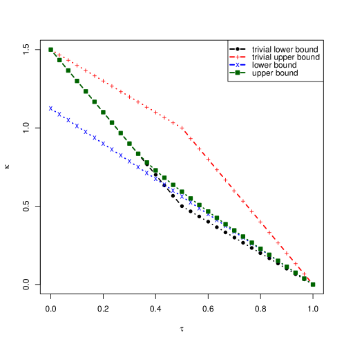
Figure 2 shows the bounds for the profile for (for this value the total number of edges is ). It shows trivial upper and lower bounds from Proposition 3, as well as our results (Theorem 4.1).
Not that our bounds are tight in two regions:
-
•
if , then our upper bound is equal to the trivial lower bound;
-
•
if , then our upper bound is asymptotically equal to our lower bound.
The same bounds can be obtained for other notions of profile, so the results are directly comparable with previous work. Let us show how this can be done for Kolmogorov complexity.
Let us assume that for every a bipartite graph is fixed (and there is an algorithm computing given ). Let be some positive rational numbers. Let be the maximum number of edges covered by a rectangle with and .
Proposition 4
There exists some constant such that:
-
•
If , then for all sufficiently large for most edges there is no string such that
-
•
If is edge-transitive and , then for all sufficiently large for every edge there exists a string such that
Proof
For each we consider a rectangle where consists of strings such that and consists of strings such that (, ). The number of strings such that is less than , so the edges covered by these rectangles form a minority (-fraction); for all other pairs there is no string with described properties.
The second part of the theorem is also easy. Proposition 2 guarantees that for sufficiently large the set can be covered by rectangles of size . By exhaustive search, we can find first covering of this sort (in some natural order), and this covering is determined by , so its complexity is . Then we let be the number of the rectangle that covers a given edge . The complexity of is at most . Knowing (and the entire covering, which has complexity ) we can describe and by their numbers in and .
One can also show that a random pair generated with distribution will have a profile (in terms of complexity) within the bounds from Theorem 4 (with high probability). Indeed, the law of large number says that the number of places where and differ is close to , and for each fixed number of difference we get a uniformly random edge in for close to . It remains to note that our bounds are continuous (as functions of ).
Let us note for comparison that (a weaker) upper bound for this distribution can be obtained using conditional independence technique from [6]. It is quite involved, but it also has a form (where is an explicit (but cumbersome) function) as in Theorem 5.1. So, let us compare with (the bigger value is better) for different values of (see Fig. 3).
6 A stochastic pair with minimal profile
A pair with minimal profile is constructed in [7] using the technique developed by An. Muchnik [4], [5]. However, this construction is quite artificial and cannot be translated into Shannon information theory, because the constructed pair is not a typical object in a simple family (is not stochastic in the sense of algorithmic information theory). In this section we show how to construct a graph with minimal combinatorial profile (for graphs with given number of edges). For that we first prove (using probabilistic arguments) that such a graph exists; after that it can be found by brute-force search. This gives us a stochastic pair with minimal profile. This result was announced in [7] as an unpublished result of An. Muchnik (1958–2007) and was not published since then.
To analyze random graphs we need a version of Chernoff inequality which deals with negatively correlated random variables [11].
Theorem 6.1 (Chernoff inequality)
Let be negatively correlated binary random variables (i.e., for every we have ).
Let and . Then
Following [7], we consider (for simplicity) graphs with vertices in each part and edges. We choose a random graph of this type (i.e., uniformly choose a matrix of size with ones).
Theorem 6.2
If and , then for some the probability of the event “every rectangle in contains less than ones” is close to .
Proof
Let us choose . The entries of are negatively correlated, so the Chernoff inequality (with and ) guarantees that for a fixed rectangle of size the probability of the event “this rectangle contains more than ones” is bounded by
Therefore the probability that some rectangle has too many ones does not exceed
Since , we are done.
Remark. Note that it follows from Propositions 1 and 3 that the bounds in Theorem 6.2 are the best possible.
Another simple observation: with high probability all rows and columns of contain at most elements. Indeed, the probability that in a given row (or column) the number of ones is twice more than the expected value , is doubly exponentially small (it follows from theorem 6.1), and we have only exponentially many rows and columns.
Then we can follow the plan described above: we conclude that there is a graph with both properties and logarithmic complexity; then, using the first part of proposition 4 one can easily see that a typical edge of this graph has minimal profile in the sense explained in [7]. (The second property is needed to show that the complexities of and in a typical edge are close to .)
7 Acknowledgements
I would like to thank Andrei Romashchenko and Alexander Shen for posing the problem and for fruitful discussions, and Alex Samorodnitsky for useful advice.
References
- [1] Robert Gray and Aaron Wyner. Source coding over simple networks. Bell Systems Technical Journal, 53(9):1681–1721, 1974.
- [2] Peter Gács and János Körner. Common information is far less than mutual information. Problems of Control and Information Theory, 2(2):149–162, 1973.
- [3] Konstantin Makarychev and Yury Makarychev. Conditionally independent random variables. Preprint, 2005.
- [4] Andrej Muchnik. On the extraction of common information of two words. Pervyi vsemirnyi kongress obshchestva matematicheskoi statistiki i teorii veroyatnostei imeni Bernoulli. Tezisy, 1:453, 1986.
- [5] Andrej Muchnik. On common information. Theoretical Computer Science, 207(2):319–328, 1998.
- [6] Andrei Romashchenko. Pairs of words with nonmaterializable mutual information. Problems of Information Transmission, 36:1–18, 2000.
- [7] Alexey Chernov, Andrey Muchnik, Andrei Romashchenko, Alexander Shen, and Nikolai Vereshchagin. Upper semi-lattice of binary strings with the relation “x is simple conditional to y”. Theoretical Computer Science, 271:69–95, 2002.
- [8] Rudolf Ahlswede and Peter Gács. Spreading of Sets in Product Spaces and Hypercontraction of the Markov Operator. The Annals of Probability, 4(6):925–939, 1976.
- [9] Shlomo Hoory, Nathan Linial, and Avi Wigderson. Expander graphs and their applications. Bulletin of the AMS, 43:439–561, 2006.
- [10] Christophe Garban and Jeffrey Steif. Lectures on noise sensitivity and percolation. Preprint, 2011.
- [11] Alessandro Panconesi and Aravind Srinivasan. Randomized Distributed Edge Coloring via an Extension of the Chernoff-Hoeffding Bounds. SIAM Journal on Computing, 26(2):350–368, 1997.
Appendix 0.A Properties of
We prove properties of that were promised in Section 3.
Theorem 0.A.1
iff is non-degenerate.
Proof
Suppose is degenerate. Then there are non-trivial partitions , such that and . Consider the indicator of that maps to and — to . Then for every the following equality holds: . On the other hand by Lemma 2
since , , and is non-constant. Thus, clearly, .
Conversely, let be non-degenerate. Conside the unit sphere in . For let us define . Since , is continuous, and is compact, it remains to prove that for every . If is constant then, the inequality is obvious since is constant. If is not constant, then the inequality is true, since , so there exists such that ( is continuous in ).
Theorem 0.A.2
Let , . If and , then
| (5) |