On the Instability of the Lee-Wick Bounce

Abstract

It was recently realized Cai:2008qw that a model constructed from a Lee-Wick type scalar field theory yields, at the level of homogeneous and isotropic background cosmology, a bouncing cosmology. However, bouncing cosmologies induced by pressure-less matter are in general unstable to the addition of relativistic matter (i.e. radiation). Here we study the possibility of obtaining a bouncing cosmology if we add radiation coupled to the Lee-Wick scalar field. This coupling in principle would allow the energy to flow from radiation to matter, thus providing a drain for the radiation energy. However, we find that it takes an extremely unlikely fine tuning of the initial phases of the field configurations for a sufficient amount of radiative energy to flow into matter. For general initial conditions, the evolution leads to a singularity rather than a smooth bounce.

I Introduction

Both Standard Hawking:1973uf and Inflationary Cosmology Borde:1993xh suffer from the initial singularity problem and hence cannot yield complete descriptions of the very early universe. If one were able to construct a non-singular bouncing cosmology, this problem would obviously disappear. However, in order to have a chance to obtain such a non-singular cosmology, one must either go beyond Einstein gravity as a theory of space-time (see e.g. Mukhanov:1991zn for an early construction), or else one must make use of matter which violates the “null energy condition” (see Novello for a review of both types of approaches).

Interest in non-singular bouncing cosmologies has increased with the realization that they can lead to alternatives to inflationary cosmology as a theory for the origin of structure in the universe. A specific scenario which can arise at the level of homogeneous and isotropic cosmology is the “matter bounce” paradigm which is based on the realization Wands ; Finelli that vacuum fluctuations which exit the Hubble radius during a matter-dominated contracting phase evolve into a scale-invariant spectrum of curvature perturbations on super-Hubble scales before the bounce. The key point is that the curvature fluctuation variable $\zeta$ grows on super-Hubble scales in a contracting phase, whereas it is constant on these large scales in an expanding phase. Since long wavelength modes exit the Hubble radius earlier than short wavelength ones, they grow for a longer period of time. This provides a mechanism for reddening the initial vacuum spectrum. It turns out that a matter dominated contracting phase provides the specific boost in the power of long wavelength modes which is required in order to transform a vacuum spectrum into a scale-invariant one. Studies in the case of various non-singular bounce models models have shown that on wavelengths long compared to the duration of the bounce phase, the spectrum of fluctuations is virtually unchanged during the bounce. Thus, a scale-invariant spectrum of curvature fluctuations survives on super-Hubble scales at late times.

Provided that the bounce can occur at energy scales much below the Planck scale, non-singular cosmologies solve a key conceptual problem from which inflationary cosmology suffers, namely the “Trans-Planckian” problem for fluctuations RHBrev0 ; Martin:2000xs : If the period of inflationary expansion of space lasts for more than $70H^{-1}$, where $H$ is the Hubble expansion rate during inflation (in order to solve the key cosmological mysteries it was designed to explain, inflation has to last at least $50H^{-1}$), then the physical wavelengths of even the largest-scale fluctuation modes we see today will be even smaller than the Planck length at the beginning of inflation and thus in the “zone of ignorance” where the physics on which inflation and the theory of cosmological perturbations are based, namely Einstein gravity coupled to semiclassical field theory matter, will break down. In contrast, in a non-singular bouncing cosmology the wavelength of modes which are currently probed by cosmological observations is never much smaller than $1{\rm mm}$ (the physical wavelength of the mode which corresponds to our current Hubble radius evaluated when the temperature of the universe was $10^{16}{\rm GeV}$) and hence many orders of magnitude larger than the Planck length. Thus, the fluctuations never enter the “trans-Planckian zone of ignorance” of sub-Planck-length wavelengths.

Possibly the simplest realization of the matter bounce scenario is the “quintom bounce” model Cai:2007qw and is obtained by considering the matter sector to contain two scalar fields, one of them (the “ghost field”) having the “wrong” sign of the kinetic action. The potential of the ghost scalar field also has the opposite sign to that of regular scalar fields such that in the absence of interactions, the ghost field has a classically stable minimum. As has been noticed in Cai:2008qw , such a quintom bounce model also arises from the scalar field sector of the “Lee-Wick” (LW) Lagrangian LW which contains higher derivatives terms.

The quintom and Lee-Wick bouncing cosmologies are obtained in the following way Cai:2007qw ; Cai:2008qw : We begin in the contracting phase with both the regular and the ghost scalar field oscillating homogeneously in space about their respective vacua. We assume that the energy density is dominated by the regular matter field, and that hence the total energy density is positive. Once the amplitude of the regular scalar field exceeds the Planck scale, the field oscillations will freeze out and a slow-climb phase will begin during which the energy density of the field only grows slowly (this is the time reverse of the slow-roll phase in scalar field-driven inflation). However, the ghost field continues to oscillate and its energy density (which is negative) continues to grow in absolute value. Hence, the total energy density drops to zero, at which point the bounce occurs, as has been studied both analytically and numerically in the above-mentioned works. Note that the energy density in this bounce model scales as matter until the regular scalar field freezes out.

A major problem of bouncing cosmologies realized with matter which scales as $a^{-3}$ as a function of the scale factor $a(t)$ is the potential instability of the homogeneous and isotropic background against the effects of radiation (which scales as $a^{-4}$ and anisotropic stress which scales as $a^{-6}$ . If we simply add a non-interacting radiation component to the two scalar field system, then unless the initial energy density in radiation is tuned to be extremely small, then the radiation component will become dominant long before the bounce can arise, and will prevent the energy density in the ghost field from ever being able to become important, resulting in a Big Crunch singularity. Similarly, unless the initial energy density in anisotropic stress is very small, it will come to dominate the energy density of the universe long before the bounce is expected. The anisotropies will destabilize the homogeneous background cosmology, and will prevent a bounce. Note that at the quantum level, there is an additional severe problem for bounce models obtained with matter fields with ghost-like kinetic terms, namely the quantum instability of the vacuum (see e.g. Jeon ).

In this paper we will focus on the radiation instability problem. For the purpose of this discussion we will simply assume that anisotropic stress is absent. In a recent paper, two of us studied the possibility that a bounce could arise if radiation is supplemented with Lee-Wick radiation Karouby:2010wt . However, we showed that this hope is not realized: the addition of Lee-Wick radiation does not prevent the Big Crunch singularity from occurring. In the presence of radiation, the only hope to obtain a bounce is to introduce a coupling between radiation and ghost scalar field matter which could effectively drain energy density from the radiation field and prevent the energy density of radiation from becoming dominant. Here we study this possibility. However, at least for the specific Lagrangian which we consider, we find that a bounce only emerges for highly fine-tuned phases of the fields and their velocities in the initial conditions.

The paper is organized as follows: In Section II, we introduce the model we study, namely the scalar field sector of Lee-Wick theory coupled to radiation, and write down the general equations of motion. In Section III we set up the equations of motion linearized about the bounce background, treating the entire radiation field as an inhomogeneous fluctuation. In particular, we study the different terms which contribute to the energy-momentum tensor and identify those which could assist in obtaining a non-singular bounce. In Section IV we study the solutions of the perturbed equations of motion, and in Section V we analyze the evolution of the different terms in the energy-momentum tensor, identifying the conditions which would be required in order to obtain a non-singular bounce. We have also evolved the general equations of motion for the two inhomogeneous scalar field configurations and the classical inhomogeneous radiation field in the homogeneous background cosmology. Section VI summarizes some of the numerical results. Both the analytical and numerical results confirm that we need unnatural fine-tuning of the initial conditions in order to obtain a non-singular bounce. In the final section we offer some conclusions and discussion.

II The Model

The Lee-Wick scalar field model coupled to electromagnetic radiation is given by the following Lagrangian:

$${\cal L} = -\frac{1}{2}\partial_{\mu}\phi\partial^{\mu}\phi+\frac{1}{2M^{2}}(\partial^{2}\phi)^{2}-\frac{1}{2}m^{2}\phi^{2}-V(\phi)$$ (1)

$$-\frac{1}{4}F_{\mu\nu}F^{\mu\nu}-f(\phi,\partial^{2}\phi,F_{\mu\nu}F^{\mu\nu})~{},$$

where $m$ is the mass of the scalar field $\phi$, and $V(\phi)$ is its potential. Here we adopt the convention that

$$ds^{2}\,=\,-dt^{2}+a^{2}(t)(dx^{2}+dy^{2}+dz^{2})\,,$$ (2)

where $a(t)$ is the scale factor of the universe. Since it is a higher derivative Lagrangian in $\phi$, the scalar field sector contains an extra degree of freedom with the “wrong” sign kinetic term and with a mass set by the scale $M$. We choose $m\leq M\leq m_{Pl}$, where $m_{Pl}$ is the Planck mass, since we want the regular scalar field to dominate at low energies, but at the same time we do not want to worry about quantum gravity effects. The second line of the Lagrangian (1) contains the kinetic term of the radiation as well as the coupling term, where we assumed both for the sake of generality and because of foresight that the radiation field couples not only to the scalar field $\phi$ itself, but also to the higher derivative term. The electromagnetic tensor, $F_{\mu\nu}$, is related to the radiation field $A_{\mu}$ through the usual definition

$$F_{\mu\nu}\,\equiv\,\nabla_{\mu}A_{\nu}-\nabla_{\nu}A_{\mu}\,,$$ (3)

where $\nabla_{\mu}$ is the covariant derivative.

It is convenient to extract the extra degree of freedom as a separate scalar field. To do this, we use the field redefinitions

$$\phi\, \equiv \,\phi_{1}-\phi_{2}\,,$$

$$\phi_{2}\, \equiv \,\partial^{2}\phi/M^{2}\,.$$ (4)

The Lagrangian (1) then takes on a simpler form:

$${\cal L}\, = \,-\frac{1}{2}\partial_{\mu}\phi_{1}\partial^{\mu}\phi_{1}+\frac{1}{2}\partial_{\mu}\phi_{2}\partial^{\mu}\phi_{2}-\frac{1}{2}m^{2}\phi_{1}^{2}+\frac{1}{2}M^{2}\phi_{2}^{2}\,$$ (5)

$$\,-\frac{1}{4}F_{\mu\nu}F^{\mu\nu}-f(\phi_{1},\phi_{2},F_{\mu\nu}F^{\mu\nu})~{},$$

where we have chosen the potential to be zero. In this new form, the Lagrangian describes two massive scalar fields with one of them (i.e., $\phi_{2}$) behaving like a“ghost”, and both of them coupled to the radiation field.

The coupling term $f(\phi_{1},\phi_{2},F_{\mu\nu}F^{\mu\nu})$ should in principle be arbitrary, however, in this paper we will take a specific form for convenience. The form will be:

$$f(\phi_{1},\phi_{2},F_{\mu\nu}F^{\mu\nu})\,=\,\frac{1}{4}(c\phi_{1}^{2}+d\phi_{2}^{2})F_{\mu\nu}F^{\mu\nu}~{},$$ (6)

where $c$ and $d$ are coupling constants which have mass dimension $-2$. The interaction terms are non-renormalizable. To make sure that such terms could be thought of as arising from an effective field theory which is consistent at the bounce, we must make sure that the coefficients are chosen such that the contribution of the interaction term to the Lagrangian density is smaller than that of the other terms. This must be true even at energy densities at which the bounce occurs in the pure scalar field model. It is easy to see that this condition will be satisfied if the coefficients $c$ and $d$ are both of the order $m_{pl}^{-2}$.

It is the purpose of this paper to study the effects which these coupling terms have on the dynamics of the system. We know that in the absence of coupling, i.e. when $c=d=0$, a bounce will only occur if the initial radiation energy density is tuned to a very small value compared to the scalar field energy density. This is because the positive definite energy density of radiation will scale as $a^{-4}$ which is faster than that of the scalar fields, in particular the ghost scalar field. Generically, it will dominate the energy of the universe after some amount of contraction, it will prevent the ghost scalar field energy density from catching up and will thus prevent a bounce, leading to a Big Crunch singularity instead. With non-vanishing values of $c$ and $d$, however, the scalars are in principle able to drain energy from the radiation.

From the Lagrangian (5), one can obtain the stress-energy tensor $T_{\mu\nu}$ by varying the action with respect to the metric $g^{\mu\nu}$. In the hydrodynamical limit, we can take $T_{\mu\nu}$ to be of the form of $diag\{\rho,a^{2}(t)p_{1},a^{2}(t)p_{2},a^{2}(t)p_{3}\}$ where $\rho$ and $p$ are energy density and pressure, respectively. For now, we consider the general form which is:

$$T_{\mu\nu} = g_{\mu\nu}{\cal L}+\partial_{\mu}\phi_{1}\partial_{\nu}\phi_{1}-\partial_{\mu}\phi_{2}\partial_{\nu}\phi_{2}+(1-c\phi_{1}^{2}-d\phi_{2}^{2})F_{\mu\lambda}F_{\nu}^{\lambda}~{},$$ (7)

$$= g_{\mu\nu}\bigl{[}\frac{\dot{\phi}_{1}^{2}}{2}-\frac{1}{2a^{2}}\partial_{i}\phi_{1}\partial_{i}\phi_{1}-\frac{1}{2}m^{2}\phi_{1}^{2}-\frac{\dot{\phi}_{2}^{2}}{2}+\frac{1}{2a^{2}}\partial_{i}\phi_{2}\partial_{i}\phi_{2}+\frac{1}{2}M^{2}\phi_{2}^{2}-\frac{1}{4}(1-c\phi_{1}^{2}-d\phi_{2}^{2})F^{2}\bigr{]}~{}$$

$$+\partial_{\mu}\phi_{1}\partial_{\nu}\phi_{1}-\partial_{\mu}\phi_{2}\partial_{\nu}\phi_{2}+(1-c\phi_{1}^{2}-d\phi_{2}^{2})F_{\mu\lambda}F_{\nu}^{\lambda}~{}.$$

Since we will be studying the contribution of plane wave perturbations of the scalar fields and we will treat radiation as a superposition of waves, we kept the space-derivative terms.

By varying the Lagrangian with respect to the matter fields $\phi_{1}$, $\phi_{2}$ and $A_{\mu}$, we also get the equations of motion for all three fields:

$$\Box\phi_{1}-(m^{2}-\frac{c}{2}F^{2})\phi_{1}=0~{},$$ (8)

$$\Box\phi_{2}-(M^{2}+\frac{d}{2}F^{2})\phi_{2}=0~{},$$ (9)

$$(1-c\phi_{1}^{2}-d\phi_{2}^{2})(\partial_{\nu}F^{\mu\nu}+3HF^{\mu 0})$$

$$-2(c\phi_{1}\partial_{\nu}\phi_{1}+d\phi_{2}\partial_{\nu}\phi_{2})F^{\mu\nu}=0~{}$$ (10)

which will be analyzed in detail in the rest of the paper.

III Dynamics

Since the equations of motion are nonlinear, we cannot work in Fourier space, and use plane wave solutions. However, we are interested in how initially small amounts of radiation build up and possibly transfer their energy to scalar field fluctuations. We treat radiation as a superposition of fluctuations. Therefore it makes sense to linearize our equations about the homogeneous scalar field background. Thus, we make the following ansatz for the scalar fields:

$$\phi_{1}(t,z) = \phi_{1}^{(0)}(t)+\epsilon\phi_{1}^{(1)}(t,z)+\epsilon^{2}\phi_{1}^{(2)}(t)$$ (11)

$$\phi_{2}(t,z) = \phi_{2}^{(0)}(t)+\epsilon\phi_{2}^{(1)}(t,z)+\epsilon^{2}\phi_{2}^{(2)}(t)~{},$$ (12)

where the expansion parameter $\epsilon$ is taken to be much smaller than $1$ . The first term on the right hand side of each line, i.e. $\phi_{1,2}^{(0)}(t)$ correspond to the background fields, the terms $\phi_{1,2}^{(1)}(t,x)$ are the fluctuations, and the second order terms $\phi_{1,2}^{(2)}(t)$ describe the back-reaction of the fluctuations on the background and can be computed from the leading second order corrections (averaged over space) of the equations of motion .

To simplify the analysis, we describe radiation in terms of plane waves in a fixed direction (which we take to be the $z$ direction). Without loss of generality we can restrict attention to one polarization mode which we take to be the electric field in the $x$ direction and the magnetic field in the $y$ direction. In this case, the only non-zero components of the field strength tensor are $F^{01}$ and $F^{13}$. Using the temporal gauge where $A_{0}=0$, we find that only the first component of the gauge field is non-zero. For a single wavelength fluctuation we can make the ansatz

$$A_{1}(k,t)\,=\,f(t)cos(kz)\equiv\gamma(k,t)~{},$$ (13)

or, equivalently,

$$A^{1}(k,t)\,=\,a(t)^{-2}\gamma(k,t)~{}.$$ (14)

Since in the linearized equations of motion the Fourier modes are independent, we can consider $\phi_{1}^{(1)}$ and $\phi_{2}^{(1)}$ also to be plane waves propagating in $z$ direction, so they depend only on $z$ and $t$.

With Eqs. (11-14) in hand, we can write down the energy densities of the various fields at each order in perturbation theory.

III.1 The stress-energy tensor

First of all, we insert the above perturbative ansatz for the fields into the stress-energy tensor of the system. From the general expression (7) for $T_{\mu\nu}$ we get:

$$T_{\mu\nu} = g_{\mu\nu}\bigl{[}\frac{\dot{\phi}_{1}^{2}}{2}-\frac{1}{2a^{2}}\partial_{z}\phi_{1}\partial_{z}\phi_{1}-\frac{1}{2}m^{2}\phi_{1}^{2}-\frac{\dot{\phi}_{2}^{2}}{2}+\frac{1}{2a^{2}}\partial_{z}\phi_{2}\partial_{z}\phi_{2}+\frac{1}{2}M^{2}\phi_{2}^{2}-\frac{1}{4}(1-c\phi_{1}^{2}-d\phi_{2}^{2})F^{2}\bigr{]}~{}$$ (15)

$$+\partial_{\mu}\phi_{1}\partial_{\nu}\phi_{1}-\partial_{\mu}\phi_{2}\partial_{\nu}\phi_{2}+(1-c\phi_{1}^{2}-d\phi_{2}^{2})F_{\mu\lambda}F_{\nu}^{\lambda}~{}.$$

The $00$ component of Eq. (15) denotes the energy density of the system:

$$\rho = \frac{1}{2}(\dot{\phi}_{1}^{2}+\frac{k^{2}}{a^{2}}\phi_{1}^{2}+m^{2}\phi_{1}^{2})-\frac{1}{2}(\dot{\phi}_{2}^{2}+\frac{k^{2}}{a^{2}}\phi_{2}^{2}+M^{2}\phi_{2}^{2})$$ (16)

$$+(1-c\phi_{1}^{2}-d\phi_{2}^{2})(\frac{F^{2}}{4}+F_{0\lambda}F_{0}^{\lambda})~{},$$

so at each level in perturbation theory we have:

$$\rho^{(0)} = \frac{1}{2}(\dot{\phi_{1}^{(0)}}^{2}+m^{2}{\phi_{1}^{(0)}}^{2})-\frac{1}{2}(\dot{\phi_{2}^{(0)}}^{2}+M^{2}{\phi_{2}^{(0)}}^{2})~{},$$ (17)

$$\rho^{(1)} = (\dot{\phi}_{1}^{(0)}\dot{\phi}_{1}^{(1)}+m^{2}\phi_{1}^{(0)}\phi_{1}^{(1)})-(\dot{\phi}_{2}^{(0)}\dot{\phi}_{2}^{(1)}$$ (18)

$$+M^{2}\phi_{2}^{(0)}\phi_{2}^{(1)})~{},$$

$$\rho^{(2)} = \frac{1}{2}(\dot{\phi_{1}^{(1)}}^{2}+\dot{\phi}_{1}^{(0)}\dot{\phi}_{1}^{(2)}+\frac{k^{2}}{a^{2}}{\phi_{1}^{(1)}}^{2}+m^{2}{\phi_{1}^{(1)}}^{2}$$ (19)

$$+m^{2}\phi_{1}^{(0)}\phi_{1}^{(2)})-\frac{1}{2}(\dot{\phi_{2}^{(1)}}^{2}+\dot{\phi}_{2}^{(0)}\dot{\phi}_{2}^{(2)}+\frac{k^{2}}{a^{2}}{\phi_{2}^{(1)}}^{2}$$

$$+M^{2}{\phi_{2}^{(1)}}^{2}+M^{2}\phi_{2}^{(0)}\phi_{2}^{(2)})$$

$$+(1-c{\phi_{1}^{(0)}}^{2}-d{\phi_{2}^{(0)}}^{2})(\frac{F^{2}}{4}+F_{0\lambda}F_{0}^{\lambda})~{},$$

$$= \frac{1}{2}(\dot{\phi_{1}^{(1)}}^{2}+\dot{\phi}_{1}^{(0)}\dot{\phi}_{1}^{(2)}+\frac{k^{2}}{a^{2}}{\phi_{1}^{(1)}}^{2}+m^{2}{\phi_{1}^{(1)}}^{2}$$

$$+m^{2}\phi_{1}^{(0)}\phi_{1}^{(2)})-\frac{1}{2}(\dot{\phi_{2}^{(1)}}^{2}+\dot{\phi}_{2}^{(0)}\dot{\phi}_{2}^{(2)}+\frac{k^{2}}{a^{2}}{\phi_{2}^{(1)}}^{2}$$

$$+M^{2}{\phi_{2}^{(1)}}^{2}+M^{2}\phi_{2}^{(0)}\phi_{2}^{(2)})$$

$$+(1-c{\phi_{1}^{(0)}}^{2}-d{\phi_{2}^{(0)}}^{2})(\frac{k^{2}}{2a^{4}}\gamma^{2}+\frac{\dot{\gamma}^{2}}{2a^{2}})~{}.$$

We can similarly obtain the pressure of the system from the $ii$ components of Eq. (15). Note that due to the anisotropy in $T_{\mu\nu}$ caused by the gauge field as well as by the anisotropic fluctuations of the scalar fields, the pressures in the three directions are no longer identical. The pressure in each direction can be written as:

$$p_{i} = \frac{1}{2}(\dot{\phi}_{1}^{2}-\frac{k^{2}}{a^{2}}\phi_{1}^{2}-m^{2}\phi_{1}^{2})-\frac{1}{2}(\dot{\phi}_{2}^{2}-\frac{k^{2}}{a^{2}}\phi_{2}^{2}-M^{2}\phi_{2}^{2})$$ (20)

$$-(1-c\phi_{1}^{2}-d\phi_{2}^{2})(\frac{F^{2}}{4}-\frac{F_{i\lambda}F_{i}^{\lambda}}{a^{2}})+\frac{\partial_{i}\phi_{1}\partial_{i}\phi_{1}}{a^{2}}$$

$$-\frac{\partial_{i}\phi_{2}\partial_{i}\phi_{2}}{a^{2}}~{},$$

with no summation over the index $i$. From this formula, we can see that at both zero-th and first order, the pressure is isotropic:

$$p_{i}^{(0)} = \frac{1}{2}(\dot{\phi_{1}^{(0)}}^{2}-m^{2}{\phi_{1}^{(0)}}^{2})-\frac{1}{2}(\dot{\phi_{2}^{(0)}}^{2}-M^{2}{\phi_{2}^{(0)}}^{2})~{},$$ (21)

$$p_{i}^{(1)} = (\dot{\phi}_{1}^{(0)}\dot{\phi}_{1}^{(1)}-m^{2}\phi_{1}^{(0)}\phi_{1}^{(1)})-(\dot{\phi}_{2}^{(0)}\dot{\phi}_{2}^{(1)}$$ (22)

$$-M^{2}\phi_{2}^{(0)}\phi_{2}^{(1)})~{},$$

while the second order pressure for each direction gives

$$p_{i}^{(2)} = \frac{1}{2}(\dot{\phi_{1}^{(1)}}^{2}+\dot{\phi}_{1}^{(0)}\dot{\phi}_{1}^{(2)}-\frac{k^{2}}{a^{2}}{\phi_{1}^{(1)}}^{2}+m^{2}{\phi_{1}^{(1)}}^{2}$$ (23)

$$+m^{2}\phi_{1}^{(0)}\phi_{1}^{(2)})-\frac{1}{2}(\dot{\phi_{2}^{(1)}}^{2}+\dot{\phi}_{2}^{(0)}\dot{\phi}_{2}^{(2)}-\frac{k^{2}}{a^{2}}{\phi_{2}^{(1)}}^{2}$$

$$+M^{2}{\phi_{2}^{(1)}}^{2}+M^{2}\phi_{2}^{(0)}\phi_{2}^{(2)})+\frac{\partial_{i}\phi_{1}\partial_{i}\phi_{1}}{a^{2}}-\frac{\partial_{i}\phi_{2}\partial_{i}\phi_{2}}{a^{2}}$$

$$-(1-c{\phi_{1}^{(0)}}^{2}-d{\phi_{2}^{(0)}}^{2})(\frac{F^{2}}{4}-\frac{F_{i\lambda}F_{i}^{\lambda}}{a^{2}})~{},$$

where $i=1,2,3$.

We can thus obtain every component of $p_{i}^{(2)}$:

$$p_{1}^{(2)} = \frac{1}{2}(\dot{\phi_{1}^{(1)}}^{2}+\dot{\phi}_{1}^{(0)}\dot{\phi}_{1}^{(2)}-\frac{k^{2}}{a^{2}}{\phi_{1}^{(1)}}^{2}+m^{2}{\phi_{1}^{(1)}}^{2}$$ (24)

$$+m^{2}\phi_{1}^{(0)}\phi_{1}^{(2)})-\frac{1}{2}(\dot{\phi_{2}^{(1)}}^{2}+\dot{\phi}_{2}^{(0)}\dot{\phi}_{2}^{(2)}-\frac{k^{2}}{a^{2}}{\phi_{2}^{(1)}}^{2}$$

$$+M^{2}{\phi_{2}^{(1)}}^{2}+M^{2}\phi_{2}^{(0)}\phi_{2}^{(2)})$$

$$+(1-c{\phi_{1}^{(0)}}^{2}-d{\phi_{2}^{(0)}}^{2})(\frac{k^{2}}{2a^{4}}\gamma^{2}-\frac{\dot{\gamma}^{2}}{2a^{2}})~{},$$

$$p_{2}^{(2)} = \frac{1}{2}(\dot{\phi_{1}^{(1)}}^{2}+\dot{\phi}_{1}^{(0)}\dot{\phi}_{1}^{(2)}-\frac{k^{2}}{a^{2}}{\phi_{1}^{(1)}}^{2}+m^{2}{\phi_{1}^{(1)}}^{2}$$ (25)

$$+m^{2}\phi_{1}^{(0)}\phi_{1}^{(2)})-\frac{1}{2}(\dot{\phi_{2}^{(1)}}^{2}+\dot{\phi}_{2}^{(0)}\dot{\phi}_{2}^{(2)}-\frac{k^{2}}{a^{2}}{\phi_{2}^{(1)}}^{2}$$

$$+M^{2}{\phi_{2}^{(1)}}^{2}+M^{2}\phi_{2}^{(0)}\phi_{2}^{(2)})$$

$$-(1-c{\phi_{1}^{(0)}}^{2}-d{\phi_{2}^{(0)}}^{2})(\frac{k^{2}}{2a^{4}}\gamma^{2}-\frac{\dot{\gamma}^{2}}{2a^{2}})~{},$$

$$p_{3}^{(2)} = \frac{1}{2}(\dot{\phi_{1}^{(1)}}^{2}+\dot{\phi}_{1}^{(0)}\dot{\phi}_{1}^{(2)}-\frac{k^{2}}{a^{2}}{\phi_{1}^{(1)}}^{2}+m^{2}{\phi_{1}^{(1)}}^{2}$$ (26)

$$+m^{2}\phi_{1}^{(0)}\phi_{1}^{(2)})-\frac{1}{2}(\dot{\phi_{2}^{(1)}}^{2}+\dot{\phi}_{2}^{(0)}\dot{\phi}_{2}^{(2)}-\frac{k^{2}}{a^{2}}{\phi_{2}^{(1)}}^{2}$$

$$+M^{2}{\phi_{2}^{(1)}}^{2}+M^{2}\phi_{2}^{(0)}\phi_{2}^{(2)})$$

$$+(1-c{\phi_{1}^{(0)}}^{2}-d{\phi_{2}^{(0)}}^{2})(\frac{k^{2}}{2a^{4}}\gamma^{2}+\frac{\dot{\gamma}^{2}}{2a^{2}})~{},$$

and the average is:

$$p_{eff}^{(2)} = \frac{p_{1}^{(2)}+p_{2}^{(2)}+p_{3}^{(2)}}{3}~{}$$ (28)

$$= \frac{1}{2}(\dot{\phi_{1}^{(1)}}^{2}+\dot{\phi}_{1}^{(0)}\dot{\phi}_{1}^{(2)}-\frac{k^{2}}{a^{2}}{\phi_{1}^{(1)}}^{2}+m^{2}{\phi_{1}^{(1)}}^{2}$$

$$+m^{2}\phi_{1}^{(0)}\phi_{1}^{(2)})-\frac{1}{2}(\dot{\phi_{2}^{(1)}}^{2}+\dot{\phi}_{2}^{(0)}\dot{\phi}_{2}^{(2)}-\frac{k^{2}}{a^{2}}{\phi_{2}^{(1)}}^{2}$$

$$+M^{2}{\phi_{2}^{(1)}}^{2}+M^{2}\phi_{2}^{(0)}\phi_{2}^{(2)})$$

$$+(1-c{\phi_{1}^{(0)}}^{2}-d{\phi_{2}^{(0)}}^{2})(\frac{k^{2}}{6a^{4}}\gamma^{2}+\frac{\dot{\gamma}^{2}}{6a^{2}})~{}.$$

From the above, we can also see that in order to analyze the behavior of the energy density up to second order, we need to know the evolution of scalar fields up to second order as well as that of the gauge field up to first order, while the behavior of the gauge field to second order is not required.

It will be useful in the following to separate the contributions to the energy density and pressure in a different way, namely,
i) the contribution from the background homogeneous part of the scalar fields,

$$\rho_{\phi}^{h}=\rho_{\phi}^{(0)}\,\ ~{}~{}~{}p_{\phi}^{h}=p_{\phi}^{(0)}~{},$$ (29)

ii) that of the scalar field perturbations (in slight abuse of notation we call this the “inhomogeneous” term),

$$\rho_{\phi}^{inh}=\epsilon\rho_{\phi}^{(1)}+\epsilon^{2}\rho_{\phi}^{(2)}\,~{}~{}~{}p_{\phi}^{inh}=\epsilon p_{\phi}^{(1)}+\epsilon^{2}p_{\phi}^{(2)}~{},$$ (30)

iii) the contribution of the gauge field,

$$\rho_{g} = \frac{1}{2a^{2}}(\dot{\gamma}^{2}+\frac{k^{2}}{a^{2}}\gamma^{2})~{},$$ (31)

$$p_{g} = \frac{1}{12a^{2}}(\dot{\gamma}^{2}+\frac{k^{2}}{a^{2}}\gamma^{2})~{},$$ (32)

and iv) the contribution of the coupling term,

$$\rho_{c} = -\frac{(c{\phi_{1}^{(0)}}^{2}+d{\phi_{2}^{(0)}}^{2})}{8a^{2}}(\dot{\gamma}^{2}+\frac{k^{2}}{a^{2}}\gamma^{2})=-\Phi\rho_{g}~{},$$ (33)

$$p_{c} = -\frac{(c{\phi_{1}^{(0)}}^{2}+d{\phi_{2}^{(0)}}^{2})}{24a^{2}}(\dot{\gamma}^{2}+\frac{k^{2}}{a^{2}}\gamma^{2})=-\Phi p_{g}~{},$$ (34)

where in the last equation we define $\Phi$ to be the quadratic combination of the two fields:

$$\Phi=(c{\phi_{1}^{(0)}}^{2}+d{\phi_{2}^{(0)}}^{2})/2\,.$$ (35)

From the above we can deduce the equation of state parameter for each part:

$$w_{\phi}^{h} = \frac{\dot{{\phi_{1}^{(0)}}}^{2}-m^{2}{\phi_{1}^{(0)}}^{2}-\dot{{\phi_{2}^{(0)}}}^{2}+M^{2}{\phi_{2}^{(0)}}^{2}}{\dot{{\phi_{1}^{(0)}}}^{2}+m^{2}{\phi_{1}^{(0)}}^{2}-\dot{{\phi_{2}^{(0)}}}^{2}-M^{2}{\phi_{2}^{(0)}}^{2}}~{},$$ (36)

$$w_{\phi}^{inh} = \epsilon\left(\frac{p^{(1)}}{\rho^{(1)}}-\frac{p^{(0)}\rho^{(1)}}{{\rho^{(0)}}^{2}}\right)$$ (37)

$$+\epsilon^{2}\left(\frac{p^{(2)}}{\rho^{(0)}}-\frac{p^{(0)}\rho^{(2)}}{{\rho^{(0)}}^{2}}-\frac{p^{(1)}\rho^{(1)}}{{\rho^{(0)}}^{2}}\right)~{},$$

$$w_{g} = w_{c}=\frac{1}{3}~{}.$$ (38)

From the equations above, we see that for positive values of the constants $c$ and $d$, the coupling of the scalar field with the gauge field will give rise to a contribution $\rho_{c}$ to the energy density which has the same equation of state but opposite sign to that of the gauge field. Therefore the coupling can help drain energy from the gauge field. It is because of this mechanism that we might hope to achieve a cosmological bounce in the presence of radiation. A first indication on whether a bounce might occur can be obtained by considering the scaling of each contribution to the energy density as a function of the scale factor $a(t)$. To find these scalings, we need the time dependence of the linear and quadratic contributions to each field. Therefore, we need to solve the matter field equations of motion. In the following subsection, we present the equations for the fields at each order, while the solutions and detailed analysis will be performed in the next sections.

III.2 Equations of Motion

Keeping in mind the ansätze for $A_{\mu}$, $\phi_{1}$ and $\phi_{2}$, their equations of motion at each order can be obtained from (8), (9) and (II):
a) At zero-th order:

$$\left\{\begin{array}[]{c}\ddot{\phi}_{1}^{(0)}+3H\dot{\phi}_{1}^{(0)}+m^{2}\phi_{1}^{(0)}=0~{},\\ \\ \ddot{\phi}_{2}^{(0)}+3H\dot{\phi}_{2}^{(0)}+M^{2}\phi_{2}^{(0)}=0~{}.\\ \end{array}\right.$$ (42)

Note that there is no equation at this order for $A_{\mu}$ because it is of first order in $\epsilon$.
b) At first order:

$$\left\{\begin{array}[]{c}\ddot{\phi}_{1}^{(1)}+3H\dot{\phi}_{1}^{(1)}+(\frac{k^{2}}{a^{2}}+m^{2})\phi_{1}^{(1)}=0~{},\\ \\ \ddot{\phi}_{2}^{(1)}+3H\dot{\phi}_{2}^{(1)}+(\frac{k^{2}}{a^{2}}+M^{2})\phi_{2}^{(1)}=0~{},\\ \\ (1-c{\phi_{1}^{(0)}}^{2}-d{\phi_{2}^{(0)}}^{2})(\partial_{\nu}F^{\mu\nu}+3HF^{\mu 0})\\ -2(c\phi_{1}^{(0)}\partial_{\nu}\phi_{1}^{(0)}+d\phi_{2}^{(0)}\partial_{\nu}\phi_{2}^{(0)})F^{\mu\nu}=0~{},\\ \end{array}\right.$$ (49)

Making use of Eqs. (13) and (14), the equation for the gauge field can also be rewritten as:

$$(1-c{\phi_{1}^{(0)}}^{2}-d{\phi_{2}^{(0)}}^{2})(\ddot{\gamma}+H\dot{\gamma}+\frac{k^{2}}{a^{2}}\gamma)$$

$$-2(c\phi_{1}^{(0)}\dot{\phi}_{1}^{(0)}+d\phi_{2}^{(0)}\dot{\phi}_{2}^{(0)})\dot{\gamma}=0~{}.$$ (50)

c) At second order:

$$\left\{\begin{array}[]{c}\ddot{\phi}_{1}^{(2)}+m^{2}\phi_{1}^{(2)}-\frac{c}{2}<F_{\mu\nu}F^{\mu\nu}>\phi_{1}^{(0)}=0~{},\\ \\ \ddot{\phi}_{2}^{(2)}+M^{2}\phi_{2}^{(2)}+\frac{d}{2}<F_{\mu\nu}F^{\mu\nu}>\phi_{2}^{(0)}=0~{}.\\ \end{array}\right.$$ (54)

Here, pointed parentheses indicate spatial averaging (since we are only focusing on the zero mode of the second order field fluctuations). We also neglected the effect of Hubble friction since it does not give an important contribution for the second order fluctuations.

IV The general solution

In this section we will solve the equations of motion (42), (49) and (54) to see if and how a bounce will happen.

It is usually useful to perform the analysis in the conformal frame where the conformal time $\eta\equiv\int a^{-1}(t)dt$ is used rather than the cosmic time. Additionally, to extract the dependence on the scale factor, it is convenient to use the following two variables:

$$u_{1}(\eta)\equiv a(\eta)\phi_{1}(\eta),~{}~{}~{}u_{2}(\eta)\equiv a(\eta)\phi_{2}(\eta)~{}.$$ (55)

Hereafter, we will use $u^{(i)}_{j}(i=0,1,2,~{}j=1,2)$ to denote the $i$-th order perturbation of the $j$-th scalar field. Moreover, for simplicity but without loosing generality, we can parameterize the scale factor $a(t)$ as

$$a(\eta)=a_{0}t^{p}=a_{0}|\eta|^{\frac{p}{1-p}}~{},$$ (56)

with

$$p=\frac{2}{3(1+w)}~{},$$ (57)

where $a_{0}$ and $w$ are the initial value of the scale factor and the equation of state of the universe, respectively. This is a self-consistent assumption when $w$ is nearly a constant. The evolution of $w$ in our case will be shown numerically in Section VI.

IV.1 Solutions for $\phi_{1}^{(0)}$ and $\phi_{2}^{(0)}$

Using the parametrization (56), the equations of motion at zeroth order of the two scalar fields become:

$$\left\{\begin{array}[]{c}{u_{1}^{(0)}}^{\prime\prime}+(a_{0}^{2}m^{2}\eta^{\frac{2p}{1-p}}-\frac{p(2p-1)}{(1-p)^{2}\eta^{2}})u_{1}^{(0)}=0~{},\\ \\ {u_{2}^{(0)}}^{\prime\prime}+(a_{0}^{2}M^{2}\eta^{\frac{2p}{1-p}}-\frac{p(2p-1)}{(1-p)^{2}\eta^{2}})u_{2}^{(0)}=0~{},\\ \end{array}\right.$$ (61)

where a prime denotes the derivative with respect to conformal time $\eta$. Their solutions are:

$$u_{1}^{(0)} \sim \sqrt{|\eta|}H_{\pm\frac{1-3p}{2}}\bigl{(}(1-p)am|\eta|\bigr{)}~{},$$ (62)

$$u_{2}^{(0)} \sim \sqrt{|\eta|}H_{\pm\frac{1-3p}{2}}\bigl{(}(1-p)aM|\eta|\bigr{)}~{},$$ (63)

where $H_{\pm\frac{1-3p}{2}}$ represents the $(\pm\frac{1-3p}{2})$-th order Hankel function. Far away or close to the bounce, i.e. for $a|\eta|\gg m^{-1},M^{-1}$ and $a|\eta|\ll m^{-1},M^{-1}$, respectively, the approximate solutions are:
1)Oscillations for large values of the scale factor $a|\eta|\gg m^{-1},M^{-1}$:

$$u_{1}^{(0)} \sim |\eta|^{\frac{p}{2(p-1)}}\sqrt{\frac{2}{(1-p)\pi a_{0}m}}\cos\bigl{(}(1-p)a_{0}m|\eta|^{\frac{1}{1-p}}$$ (64)

$$+\theta_{1}^{(0)}\bigr{)}~{},$$

$$u_{2}^{(0)} \sim |\eta|^{\frac{p}{2(p-1)}}\sqrt{\frac{2}{(1-p)\pi a_{0}M}}\cos\bigl{(}(1-p)a_{0}M|\eta|^{\frac{1}{1-p}}$$ (65)

$$+\theta_{2}^{(0)}\bigr{)}~{},$$

(where $\theta_{1}$ and $\theta_{2}$ are phases set by the initial conditions). In terms of the non-rescaled fields $\phi_{i}$ one obtains damped (or anti-damped) oscillations (depending on whether we are in an expanding or a contracting period)

$$\phi_{1}^{(0)} \sim |\eta|^{\frac{3p}{2(p-1)}}\sqrt{\frac{2}{(1-p)\pi a^{\frac{3}{2}}_{0}m}}\cos\bigl{(}(1-p)a_{0}m|\eta|^{\frac{1}{1-p}}$$ (66)

$$+\theta_{1}^{(0)}\bigr{)}~{},$$

$$\phi_{2}^{(0)} \sim |\eta|^{\frac{3p}{2(p-1)}}\sqrt{\frac{2}{(1-p)\pi a^{\frac{3}{2}}_{0}M}}\cos\bigl{(}(1-p)a_{0}M|\eta|^{\frac{1}{1-p}}$$ (67)

$$+\theta_{2}^{(0)}\bigr{)}~{}.$$

2)“Frozen” evolution for small values of the scale factor $a|\eta|\ll m^{-1},M^{-1}$:

$$u_{1}^{(0)} \sim \frac{\bigl{(}(1-p)a_{0}m\bigr{)}^{\frac{1-3p}{2}}|\eta|^{\frac{1-2p}{1-p}}}{\Gamma(\frac{3(1-p)}{2})}$$ (68)

$$+\frac{\bigl{(}(1-p)a_{0}m\bigr{)}^{-\frac{1-3p}{2}}|\eta|^{\frac{p}{1-p}}}{\Gamma(\frac{1+3p}{2})}~{},$$

$$u_{2}^{(0)} \sim \frac{\bigl{(}(1-p)a_{0}M\bigr{)}^{\frac{1-3p}{2}}|\eta|^{\frac{1-2p}{1-p}}}{\Gamma(\frac{3(1-p)}{2})}$$ (69)

$$+\frac{\bigl{(}(1-p)a_{0}M\bigr{)}^{-\frac{1-3p}{2}}|\eta|^{\frac{p}{1-p}}}{\Gamma(\frac{1+3p}{2})}~{},$$

from which it follows that the non-rescaled fields $\phi_{i}$ evolve as

$$\phi_{1}^{(0)} \sim \frac{\bigl{(}(1-p)a_{0}m\bigr{)}^{\frac{1-3p}{2}}|\eta|^{\frac{1-3p}{1-p}}}{a_{0}\Gamma(\frac{3(1-p)}{2})}$$ (70)

$$+\frac{\bigl{(}(1-p)a_{0}m\bigr{)}^{\frac{3p-1}{2}}}{a_{0}\Gamma(\frac{1+3p}{2})}~{},$$

$$\phi_{2}^{(0)} \sim \frac{\bigl{(}(1-p)a_{0}M\bigr{)}^{\frac{1-3p}{2}}|\eta|^{\frac{1-3p}{1-p}}}{a_{0}\Gamma(\frac{3(1-p)}{2})}$$ (71)

$$+\frac{\bigl{(}(1-p)a_{0}M\bigr{)}^{\frac{3p-1}{2}}}{a_{0}\Gamma(\frac{1+3p}{2})}~{},$$

from which we can see that the last term of $\phi_{i}^{(0)}$ is a constant mode while the first term is a varying one. Depending on the value of $p$ (or equivalently $w$) the varying mode could be growing (for $p>1/3$ or $-1<w<1$), in which case it becomes dominant, or decaying (for $p<1/3$ or $w>1/w<-1$), in which case it becomes subdominant. We can usually neglect the decaying part of the fields.

IV.2 Solutions for $\phi_{1}^{(1)}$ and $\phi_{2}^{(1)}$

Following the steps performed in the last subsection, we can also get the solutions for the first order components of the scalar fields. Using the equations (49) for the first order perturbations we obtain the following equations of motion for $u_{1}^{(1)}$ and $u_{2}^{(1)}$:

$$\left\{\begin{array}[]{c}{u_{1}^{(1)}}^{\prime\prime}+(k^{2}+a_{0}^{2}m^{2}\eta^{\frac{2p}{1-p}}-\frac{p(2p-1)}{(1-p)^{2}\eta^{2}})u_{1}^{(1)}=0~{},\\ \\ {u_{2}^{(1)}}^{\prime\prime}+(k^{2}+a_{0}^{2}M^{2}\eta^{\frac{2p}{1-p}}-\frac{p(2p-1)}{(1-p)^{2}\eta^{2}})u_{2}^{(1)}=0~{}.\\ \end{array}\right.$$ (75)

Depending on the value of $k$, we obtain different approximation solutions. For wavenumbers large compared both to the Hubble radius and to the mass term, we obtain oscillatory solutions with fixed amplitude.

Considering now modes which are still sub-Hubble (i.e. $k|\eta|>1$) but for which the mass term dominates over the contribution of the field tension (i.e. the term involving $k$), we can neglect both the $k^{2}$ term and the term involving $\frac{p(2p-1)}{(1-p)^{2}\eta^{2}}$. The simplified equation for these modes is:

$$\left\{\begin{array}[]{c}{u_{1}^{(1)}}^{\prime\prime}+a_{0}^{2}m^{2}\eta^{\frac{2p}{1-p}}u_{1}^{(1)}=0~{},\\ \\ {u_{2}^{(1)}}^{\prime\prime}+a_{0}^{2}M^{2}\eta^{\frac{2p}{1-p}}u_{2}^{(1)}=0~{},\\ \end{array}\right.$$ (79)

whose solutions are:

$$u_{1}^{(1)} \sim \sqrt{|\eta|}H_{\frac{1-p}{2}}\bigl{(}(1-p)a_{0}m|\eta|\bigr{)}$$ (80)

$$\sim |\eta|^{\frac{p}{2(p-1)}}\sqrt{\frac{2}{(1-p)\pi ma_{0}}}\cos\bigl{(}(1-p)a_{0}m|\eta|$$

$$+\theta^{(1)}_{1}\bigr{)}~{},$$

$$u_{2}^{(1)} \sim \sqrt{|\eta|}H_{\frac{1-p}{2}}\bigl{(}(1-p)a_{0}M|\eta|\bigr{)}$$ (81)

$$\sim |\eta|^{\frac{p}{2(p-1)}}\sqrt{\frac{2}{(1-p)\pi Ma_{0}}}\cos\bigl{(}(1-p)a_{0}M|\eta|$$

$$+\theta^{(1)}_{2}\bigr{)}~{}.$$

For modes outside the Hubble radius ($k\eta\ll 1$), we have:

$$\left\{\begin{array}[]{c}{u_{1}^{(1)}}^{\prime\prime}+(a_{0}^{2}m^{2}\eta^{\frac{2p}{1-p}}-\frac{p(2p-1)}{(1-p)^{2}\eta^{2}})u_{1}^{(1)}=0~{},\\ \\ {u_{2}^{(1)}}^{\prime\prime}+(a_{0}^{2}M^{2}\eta^{\frac{2p}{1-p}}-\frac{p(2p-1)}{(1-p)^{2}\eta^{2}})u_{2}^{(1)}=0~{},\\ \end{array}\right.$$ (85)

which have the same form as Eq. (61) so their solution will be the same as given in Eqs. (68) and (69).

We have thus seen that the first order solutions for the scalar fields scale the same way with $|\eta|$ as the zeroth order solution. This is because in the small $|\eta|$ region where the $a^{\prime\prime}(t)/a(t)$ term dominates over the other ones, the equations for first order and zero-th order modes are almost the same. Thus, unless the energy density in the $u_{i}^{(1)}$ modes dominates at the initial time, it will never dominate over the background contribution from the $u_{i}^{(0)}$ terms. Thus we can conclude that the first order fluctuations of scalar fields will not prevent the bounce.

IV.3 Solution for the gauge field $\gamma$

In this section, we will analyze the gauge field $\gamma$ which is also considered to be of first order. The equation (III.2) can directly be transformed to conformal frame as:

$$\gamma^{\prime\prime}+k^{2}\gamma-\frac{2(c\phi_{1}^{(0)}{\phi_{1}^{(0)}}^{\prime}+d\phi_{2}^{(0)}{\phi_{2}^{(0)}}^{\prime})}{1-c{\phi_{1}^{(0)}}^{2}-d{\phi_{2}^{(0)}}^{2}}\gamma^{\prime}=0~{}.$$ (86)

Since the coefficients $c$ and $d$ are small, we can take the last term to be a source term. In a first order Born approximation, we can write the total solution as

$$\gamma\simeq\gamma_{0}+\delta\gamma\,,$$ (87)

where $\gamma_{0}$ is the solution for the homogeneous equation obtained by setting $c=d=0$, while $\delta\gamma$ is the leading correction term obtained by inserting $\gamma_{0}$ into the source term (the last term in (86)).

The zero-th order (homogeneous) equation is easily solved and gives

$$\gamma_{0}\sim\cos(k|\eta|+\theta_{\gamma})~{}.$$ (88)

For the first order equation, it is convenient to define

$$P(\eta)\equiv-\frac{2(c\phi_{1}^{(0)}{\phi_{1}^{(0)}}^{\prime}+d\phi_{2}^{(0)}{\phi_{2}^{(0)}}^{\prime})}{1-c{\phi_{1}^{(0)}}^{2}-d{\phi_{2}^{(0)}}^{2}}\,,$$ (89)

so that the equation becomes

$$\delta\gamma^{\prime\prime}+k^{2}\delta\gamma+P(\eta)\gamma_{0}^{\prime}=0~{},$$ (90)

where we neglected the small term $P(\eta)\delta\gamma^{\prime}$. Inserting the solution of $\gamma_{0}$ (88), we get the following equation for $\delta\gamma$:

$$\delta\gamma^{\prime\prime}+k^{2}\delta\gamma=-P(\eta)\gamma_{0}^{\prime}~{}.$$ (91)

We are interested in the scaling of $\delta\gamma$ as a function of time. For this purpose, we need to work out the scaling in time of the source term in (91). Since the solutions for $\phi_{1}^{(0)}$ and $\phi_{2}^{(0)}$ scale differently in time in the two time intervals discussed in Subsection (IV.1), it is necessary to analyze these two intervals separately.

For times obeying $a|\eta|\gg m^{-1},M^{-1}$, then by differentiating (66) and (67) with respect to $\eta$ we have:

$${\phi_{1}^{(0)}}^{\prime} \sim |\eta|^{\frac{p+2}{2(p-1)}}\sqrt{\frac{2}{(1-p)\pi a^{\frac{3}{2}}_{0}m}}$$

$$\times\bigl{[}-\frac{3p}{p-1}\cos\bigl{(}(1-p)a_{0}m|\eta|^{\frac{1}{1-p}}+\theta_{1}^{(0)}\bigr{)}$$

$$+a_{0}m|\eta|^{\frac{1}{1-p}}\sin\bigl{(}(1-p)a_{0}m|\eta|^{\frac{1}{1-p}}+\theta_{1}^{(0)}\bigr{)}\bigr{]}~{},$$

$${\phi_{2}^{(0)}}^{\prime} \sim |\eta|^{\frac{p+2}{2(p-1)}}\sqrt{\frac{2}{(1-p)\pi a^{\frac{3}{2}}_{0}M}}$$

$$\times\bigl{[}-\frac{3p}{p-1}\cos\bigl{(}(1-p)a_{0}M|\eta|^{\frac{1}{1-p}}+\theta_{1}^{(0)}\bigr{)}$$

$$+a_{0}M|\eta|^{\frac{1}{1-p}}\sin\bigl{(}(1-p)a_{0}M|\eta|^{\frac{1}{1-p}}+\theta_{1}^{(0)}\bigr{)}\bigr{]}~{}.$$

Note that $|\eta|^{\frac{1}{1-p}}\sim t$ is a decaying mode in the contracting phase and thus the last terms inside the square brackets in the above formulae can be neglected compared to the first ones. Since

$$P(\eta) = -\frac{2(c\phi_{1}^{(0)}{\phi_{1}^{(0)}}^{\prime}+d\phi_{2}^{(0)}{\phi_{2}^{(0)}}^{\prime})}{1-c{\phi_{1}^{(0)}}^{2}-d{\phi_{2}^{(0)}}^{2}}$$ (94)

$$\approx -2(c\phi_{1}^{(0)}{\phi_{1}^{(0)}}^{\prime}+d\phi_{2}^{(0)}{\phi_{2}^{(0)}}^{\prime})\,,$$

then combining all these results we get:

$$\delta\gamma\sim C_{1}|\eta|^{\frac{1-4p}{1-p}}~{}.$$ (95)

For $a|\eta|\ll m^{-1},M^{-1}$ , then differentiating (70) and (71) with respect to $\eta$ we obtain

$${\phi_{1}^{(0)}}^{\prime} \sim \frac{1-3p}{1-p}\frac{\bigl{(}(1-p)a_{0}m\bigr{)}^{\frac{1-3p}{2}}|\eta|^{\frac{-2p}{1-p}}}{a_{0}\Gamma(\frac{3(1-p)}{2})}~{},$$ (96)

$${\phi_{2}^{(0)}}^{\prime} \sim \frac{1-3p}{1-p}\frac{\bigl{(}(1-p)a_{0}M\bigr{)}^{\frac{1-3p}{2}}|\eta|^{\frac{-2p}{1-p}}}{a_{0}\Gamma(\frac{3(1-p)}{2})}~{},$$ (97)

when $p>1/3$ and

$${\phi_{1}^{(0)}}^{\prime}\sim{\phi_{2}^{(0)}}^{\prime}\approx 0$$ (98)

when $p<1/3$. Then we can solve Equation (91) to get:

$$\delta\gamma \sim C_{2}|\eta|^{\frac{3-7p}{1-p}}~{},~{}~{}~{}p>\frac{1}{3}$$

$$\delta\gamma \sim C_{3}\cos(k|\eta|+\theta_{\delta\gamma})~{}.~{}~{}~{}p<\frac{1}{3}$$ (99)

In the above expressions for $\delta\gamma$, $C_{1}$, $C_{2}$ and $C_{3}$ are complicated prefactors in front of the $\eta$-dependent terms.

In summary, we see that the interactions give only a subleading correction $\delta\gamma$ to $\gamma_{0}$.

IV.4 Solutions for $\phi_{1}^{(2)}$ and $\phi_{2}^{(2)}$

Finally, let us consider the homogeneous component of the second order fluctuations of the scalars, namely, $\phi_{1}^{(2)}$ and $\phi_{2}^{(2)}$. If we only consider the energy density up to second order, these second order field perturbations give a contribution through their coupling to the background fields. In the following we find the solutions of (54) and study the effects of the induced terms in the stress-energy tensor on a possible bounce.

Given the solution for the gauge field $\gamma$ obtained in the last subsection, it is easy to rewrite Eqs. (54) as:

$$\left\{\begin{array}[]{c}{u_{1}^{(2)}}^{\prime\prime}+a^{2}m^{2}u_{1}^{(2)}=c\frac{(k^{2}\gamma^{2}-\gamma^{\prime 2})}{a^{2}}u_{1}^{(0)}~{},\\ \\ {u_{2}^{(2)}}^{\prime\prime}+a^{2}M^{2}u_{2}^{(2)}=-d\frac{(k^{2}\gamma^{2}-\gamma^{\prime 2})}{a^{2}}u_{2}^{(0)}~{},\\ \end{array}\right.$$ (103)

where we made use of the fact that

$$F_{\mu\nu}F^{\mu\nu}=2(k^{2}\gamma^{2}-a^{2}\dot{\gamma}^{2})/a^{4}\,.$$ (104)

Equation (103) has the same form as the zero-th order equation but with a small source term generated by the interaction with the gauge field. This equation can be solved using the Born approximation (details are given in the Appendix). The general solution is the sum of the general solution of the homogeneous solution plus the solution including the source which has vanishing initial data. The inhomogeneous term is suppressed by the coupling constants $c$ and $d$ compared to the homogeneous solution, but, as shown in the Appendix, it scales as a high power of $\eta^{-1}$. Via the coupling to the background scalar fields, the above second order terms enter into the expression for the energy density to second order. The signs of the corresponding terms in the energy density are indefinite in the sense that they depend on the phases of the initial field configurations. Since it is these terms that dominate the energy density near the bounce, we find that whether a bounce occurs or not depends sensitively on the phases in the initial conditions, and that in fact in the case of many plane wave modes initially excited, a bounce requires very special phase correlations.

V Evolution of the components of the energy density

In the previous section we have solved all of the field equations up to second order in the amplitude of the fluctuations. We have found the scaling in time of each field at each order. Now we are ready to look at how all of the terms in the expression for the energy density $\rho^{(0)}$, $\rho^{(1)}$ and $\rho^{(2)}$ at various orders in perturbation theory (namely, Eqs. (17)-(19)) scale in time. This analysis is straightforward but very important if we are to determine whether a bounce is possible, since in four space-time dimensional classical Einstein Gravity with flat spatial sections a bounce can only happen when the negative terms in the energy density catch up to the positive contributions Cai:2007qw .

In the following we give a table of how each term contained in $\rho$ scales with time as the background cosmology bounce point (the bounce which is achieved in the absence of radiation and scalar field inhomogeneities) is approached. We will identify the terms which dominate in this limit. This will give us a good indication under which conditions a bounce can occur. The tables are structured as follows: the first line “Terms”, indicates which term we are considering, the next set of lines “Behavior” gives the scaling in time in the various limits and in the two relevant ranges of the parameter $p$ which indicates the equation of state, and the last line gives the sign with which the term contributes to the energy density. Note that we focus on the growing mode solution to each field (which is constant for small $\eta$ in the case $p<1/3$). We give separate tables for terms of zero-th, first and second order in $\epsilon$.

a) For terms contained in $\rho^{(0)}$:
Terms $\dot{\phi_{1}^{(0)}}^{2}$ $m^{2}{\phi_{1}^{(0)}}^{2}$ $-\dot{\phi_{2}^{(0)}}^{2}$ $-M^{2}{\phi_{2}^{(0)}}^{2}$ Behavior $a^{-3-\frac{2}{p}}\big{(}a|\eta|\gg m^{-1}\big{)}$ $a^{-6}$( $a|\eta|\ll m^{-1}$ $p>\frac{1}{3}$ ) 0 ( $a|\eta|\ll m^{-1}$ $p<\frac{1}{3}$ ) $a^{-3}\big{(}a|\eta|\gg m^{-1}\big{)}$ $a^{-6+\frac{2}{p}}$( $a|\eta|\ll m^{-1}$ $p>\frac{1}{3}$ ) $a^{0}$ ( $a|\eta|\ll m^{-1}$ $p<\frac{1}{3}$ ) $a^{-3-\frac{2}{p}}\big{(}a|\eta|\gg m^{-1}\big{)}$ $a^{-6}$( $a|\eta|\ll m^{-1}$ $p>\frac{1}{3}$ ) 0 ( $a|\eta|\ll m^{-1}$ $p<\frac{1}{3}$ ) $a^{-3}\big{(}a|\eta|\gg M^{-1}\big{)}$ $a^{-6+\frac{2}{p}}$( $a|\eta|\ll M^{-1}$ $p>\frac{1}{3}$ ) $a^{0}$ ( $a|\eta|\ll M^{-1}$ $p<\frac{1}{3}$ ) Sign Positive Definite Positive Definite Negative Definite Negative Definite

b) For terms contained in $\rho^{(1)}$:
Terms $\dot{\phi}_{1}^{(0)}\dot{\phi}_{1}^{(1)}$ $\phi_{1}^{(0)}\phi_{1}^{(1)}$ $-\dot{\phi}_{2}^{(0)}\dot{\phi}_{2}^{(1)}$ Behavior $a^{-3-\frac{2}{p}}\big{(}|\eta|\gg Max\{k^{-1},(am)^{-1}\}\big{)}$ $a^{-\frac{9}{2}-\frac{1}{p}}$( $|\eta|\in[k^{-1},(am)^{-1}]$ $p>\frac{1}{3}$ ) $a^{-6}$( $|\eta|\ll Min\{k^{-1},(am)^{-1}\}$ $p>\frac{1}{3}$ ) 0 ( $|\eta|\in[k^{-1},(am)^{-1}]$ $p<\frac{1}{3}$ ) 0 ( $|\eta|\ll Min\{k^{-1},(am)^{-1}\}$ $p<\frac{1}{3}$ ) $a^{-3}\big{(}|\eta|\gg Max\{k^{-1},(am)^{-1}\}\big{)}$ $a^{-\frac{9}{2}+\frac{1}{p}}$( $|\eta|\in[k^{-1},(am)^{-1}]$ $p>\frac{1}{3}$ ) $a^{-6+\frac{2}{p}}$( $|\eta|\ll Min\{k^{-1},(am)^{-1}\}$ $p>\frac{1}{3}$ ) $a^{-\frac{3}{2}}$ ( $|\eta|\in[k^{-1},(am)^{-1}]$ $p<\frac{1}{3}$ ) $a^{0}$ ( $|\eta|\ll Min\{k^{-1},(am)^{-1}\}$ $p<\frac{1}{3}$ ) $a^{-3-\frac{2}{p}}\big{(}|\eta|\gg Max\{k^{-1},(aM)^{-1}\}\big{)}$ $a^{-\frac{9}{2}-\frac{1}{p}}$( $|\eta|\in[k^{-1},(aM)^{-1}]$ $p>\frac{1}{3}$ ) $a^{-6}$( $|\eta|\ll Min\{k^{-1},(aM)^{-1}\}$ $p>\frac{1}{3}$ ) 0 ( $|\eta|\in[k^{-1},(aM)^{-1}]$ $p<\frac{1}{3}$ ) 0 ( $|\eta|\ll Min\{k^{-1},(aM)^{-1}\}$ $p<\frac{1}{3}$ ) Sign Indefinite Indefinite Indefinite Terms $-\phi_{2}^{(0)}\phi_{2}^{(1)}$ Behavior $a^{-3}\big{(}|\eta|\gg Max\{k^{-1},(aM)^{-1}\}\big{)}$ $a^{-\frac{9}{2}+\frac{1}{p}}$( $|\eta|\in[k^{-1},(aM)^{-1}]$ $p>\frac{1}{3}$ ) $a^{-6+\frac{2}{p}}$( $|\eta|\ll Min\{k^{-1},(aM)^{-1}\}$ $p>\frac{1}{3}$ ) $a^{-\frac{3}{2}}$ ( $|\eta|\in[k^{-1},(aM)^{-1}]$ $p<\frac{1}{3}$ ) $a^{0}$ ( $|\eta|\ll Min\{k^{-1},(aM)^{-1}\}$ $p<\frac{1}{3}$ ) Sign Indefinite These terms, however, all vanish if the energy density is defined by spatial averaging.

c) For terms contained in $\rho^{(2)}$:
Terms $\dot{\phi_{1}^{(1)}}^{2}$ $\dot{\phi}_{1}^{(0)}\dot{\phi}_{1}^{(2)}$ $\frac{k^{2}}{a^{2}}{\phi_{1}^{(1)}}^{2}$ $m^{2}{\phi_{1}^{(1)}}^{2}$ $m^{2}\phi_{1}^{(0)}\phi_{1}^{(2)}$ Behavior $a^{-3-\frac{2}{p}}\big{(}k|\eta|\gg 1\big{)}$ $a^{-6}$( $k|\eta|\ll 1$ $p>\frac{1}{3}$ ) 0 ( $k|\eta|\ll 1$ $p<\frac{1}{3}$ ) $a^{-7-\frac{1}{p}}\big{(}a|\eta|\gg m^{-1}\big{)}$ $a^{-\frac{17}{2}}$( $a|\eta|\ll m^{-1}$ $p>\frac{1}{3}$ ) 0 ( $a|\eta|\ll m^{-1}$ $p<\frac{1}{3}$ ) $a^{-5}\big{(}k|\eta|\gg 1\big{)}$ $a^{-8+\frac{2}{p}}$( $k|\eta|\ll 1$ $p>\frac{1}{3}$ ) $a^{-2}$ ( $k|\eta|\ll 1$ $p<\frac{1}{3}$ ) $a^{-3}\big{(}k|\eta|\gg 1\big{)}$ $a^{-6+\frac{2}{p}}$( $k|\eta|\ll 1$ $p>\frac{1}{3}$ ) $a^{0}$ ( $k|\eta|\ll 1$ $p<\frac{1}{3}$ ) $a^{-7+\frac{1}{p}}\big{(}a|\eta|\gg m^{-1}\big{)}$ $a^{-\frac{17}{2}+\frac{2}{p}}$( $a|\eta|\ll m^{-1}$ $p>\frac{1}{3}$ ) $a^{-\frac{11}{2}+\frac{1}{p}}$ ( $a|\eta|\ll m^{-1}$ $p<\frac{1}{3}$ ) Sign Positive Definite Indefinite Positive Definite Positive Definite Indefinite
Terms $-\dot{\phi_{2}^{(1)}}^{2}$ $-\dot{\phi}_{2}^{(0)}\dot{\phi}_{2}^{(2)}$ $\frac{k^{2}}{a^{2}}{\phi_{2}^{(1)}}^{2}$ $-M^{2}{\phi_{2}^{(1)}}^{2}$ $-M^{2}\phi_{2}^{(0)}\phi_{2}^{(2)}$ Behavior $a^{-3-\frac{2}{p}}\big{(}k|\eta|\gg 1\big{)}$ $a^{-6}$( $k|\eta|\ll 1$ $p>\frac{1}{3}$ ) 0 ( $k|\eta|\ll 1$ $p<\frac{1}{3}$ ) $a^{-7-\frac{1}{p}}\big{(}a|\eta|\gg M^{-1}\big{)}$ $a^{-\frac{17}{2}}$( $a|\eta|\ll M^{-1}$ $p>\frac{1}{3}$ ) 0 ( $a|\eta|\ll M^{-1}$ $p<\frac{1}{3}$ ) $a^{-5}\big{(}k|\eta|\gg 1\big{)}$ $a^{-8+\frac{2}{p}}$( $k|\eta|\ll 1$ $p>\frac{1}{3}$ ) $a^{-2}$ ( $k|\eta|\ll 1$ $p<\frac{1}{3}$ ) $a^{-3}\big{(}k|\eta|\gg 1\big{)}$ $a^{-6+\frac{2}{p}}$( $k|\eta|\ll 1$ $p>\frac{1}{3}$ ) $a^{0}$ ( $k|\eta|\ll 1$ $p<\frac{1}{3}$ ) $a^{-7+\frac{1}{p}}\big{(}a|\eta|\gg M^{-1}\big{)}$ $a^{-\frac{17}{2}+\frac{2}{p}}$( $a|\eta|\ll M^{-1}$ $p>\frac{1}{3}$ ) $a^{-\frac{11}{2}+\frac{1}{p}}$ ( $a|\eta|\ll M^{-1}$ $p<\frac{1}{3}$ ) Sign Negative Definite Indefinite Negative Definite Negative Definite Indefinite
Terms $a^{-4}k^{2}\gamma_{0}^{2}+a^{-2}\dot{\gamma}_{0}^{2}$ $(-c{\phi_{1}^{(0)}}^{2}-d{\phi_{2}^{(0)}}^{2})(a^{-4}k^{2}\gamma_{0}^{2}+a^{-2}\dot{\gamma}_{0}^{2})$ $a^{-4}k^{2}\gamma_{0}\delta\gamma$ $a^{-2}\dot{\gamma}\dot{\delta\gamma}$ Behavior $a^{-4}$ $a^{-7}\big{(}a|\eta|\gg m^{-1}\big{)}$ $a^{-10+\frac{2}{p}}$( $a|\eta|\ll m^{-1}$ $p>\frac{1}{3}$ ) $a^{-4}$ ( $a|\eta|\ll m^{-1}$ $p<\frac{1}{3}$ ) $a^{-8+\frac{1}{p}}\big{(}a|\eta|\gg m^{-1}\big{)}$ $a^{-11+\frac{3}{p}}$( $a|\eta|\ll m^{-1}$ $p>\frac{1}{3}$ ) $a^{-4}$ ( $a|\eta|\ll m^{-1}$ $p<\frac{1}{3}$ ) $a^{-7}\big{(}a|\eta|\gg m^{-1}\big{)}$ $a^{-10+\frac{2}{p}}$( $a|\eta|\ll m^{-1}$ $p>\frac{1}{3}$ ) $a^{-4}$ ( $a|\eta|\ll m^{-1}$ $p<\frac{1}{3}$ ) Sign Positive Definite Indefinite (Depending only on $c$ and $d$) Indefinite Indefinite These terms to not vanish upon spatial averaging.

Note that we have expressed the time dependence in terms of the dependence on the scale factor $a(t)$. At this stage, we only need to focus on the exponent of the power-law scaling. The more negative the power is, the more rapidly the term grows in a contracting phase (since $a(t)$ is decreasing with time).

As mentioned earlier, the conditions for a bounce to occur in four space-time dimensional classical Einstein gravity with flat spatial sections is that the total energy density reaches zero during the contracting phase. Thus, there needs to be a negative definite term which starts out small but grows faster than the positive definite terms due to the regular scalar field and regular radiation. In the absence of radiation and scalar field inhomogeneities, it is the contribution to the energy density of the ghost field $\phi_{2}$ which plays this role.

From the table we see that there are three kinds of terms: positive definite, negative definite and indefinite ones. The first set contains the kinetic and potential terms of the normal scalar as well as the free energy density of the gauge field, the second set is made up of the kinetic and potential terms of the ghost scalar, while the third set contains terms which arise due to the coupling terms between scalars or between scalars and gauge fields.

Looking first at the terms which are independent of the coupling term between the fields, we see from the first line of the “Behavior” set of lines in the third table that, indeed, in the presence of radiation the energy density in radiation grows faster than that in the two scalar fields, thus preventing a bounce. In the presence of coupling between the fields, however, there are terms which scale with a larger negative power of $a(t)$. The signs of some of them, however, depend on the initial phases for the linear fields $\gamma$, $\phi_{1}^{(1)}$ and $\phi_{2}^{(1)}$.

Note that the signs of the scalar coupling terms are determined by the evolution of each field and thus are hard to be identified in a general analysis. The same is true for the gauge coupling terms (the last two in the third table). However, the coupling terms between the scalar fields and the gauge field (the third to last in the third table) can be made negative/positive definite easily by setting the signs of the coefficients $c$ and $d$ to be both positive/negative.

It is reasonable to assume that the contracting phase begins with the regular scalar field dominating the energy density, and that the contribution of the Lee-Wick scalar is much smaller. For single Fourier mode initial conditions of the radiation field, this can be achieved with the appropriate choice of the initial phase (see Example 1 in the following section containing our numerical results). However, for multiple initial radiation Fourier modes excited any initial phase difference between the modes will produce a contribution with the wrong sign and will thus prevent a bounce (see Example 3 in the following section). In the presence of an infinite set of modes, the phase correlations required to obtain a bounce thus appear to have negligible measure in initial condition space. Thus, even in the presence of coupling between scalar fields and radiation, the Lee-Wick bounce is unstable.

The bounce, if it exists, will happen at a time which can be chosen to be $t=0$. Its duration (the time interval lasting from the time the Hubble radius stops decreasing in the contracting phase until when it starts expanding in the post-bounce phase) will be denoted by $\Delta t$. Since the various components of the energy density scale with different powers of $a(t)$, it is clear that the duration of the bounce will be shorter or equal to the Hubble radius $H_{\rm max}^{-1}$ (which gives the time scale on which the ratios of energy densities in different components change) at the beginning of the bounce phase. For the background bounce model, we have $H_{\rm max}\sim m$.

There are two kinds of bounces according to the duration of the bounce phase i) If the period $\Delta t\simeq m^{-1}$, the bounce will go from the time

$$t_{B^{-}}\sim-\frac{(\Delta t)}{2}\sim-\frac{1}{2m}$$ (105)

to the time

$$t_{B^{+}}\sim\frac{(\Delta t)}{2}\sim\frac{1}{2m}$$ (106)

with a low speed. We call this a “slow bounce”. In this case, the universe will enter the bounce period at the critical time $t_{c}\sim m$, and only the $a|\eta|\gg m^{-1}$ approximate solutions of the previous tables will be applicable and not ones for the interval $a|\eta|\ll m^{-1}$. ii) If the period $\Delta t\ll m^{-1}$, the bounce will happen in a very short time with very fast speed. This can be called the “fast bounce”. In this case, the universe evolves from the far past ($-t_{i}$ with $|t_{i}|\gg 1$) to $t=0$, passing through the point $t_{c}\sim m$, then entering into the region $|t|\lesssim m$ before finally reaching the bounce point. In this case, both of the two approximate solutions of the field evolution will be applied.

Let us now consider the necessary conditions for a bounce (as we have indicated above and will see from the numerical analysis, these conditions are not sufficient - in addition to the conditions which follow, appropriate correlations in the initial phases are required). We start in the region of time $a|\eta|\gg m^{-1}$. We study the conditions required to have the terms that might give a bounce grow relative to the other terms during this phase. If the conditions are not satisfied, or the bounce does not happen even if the conditions are satisfied, then a bounce may still occure in the $a|\eta|\ll m^{-1}$ region. The conditions for the terms in the energy which could compensate the positive radiation contribution to become dominant are then studied. If these conditions are not satisfied, either, then a bounce is impossible.

A necessary condition for a bounce to be possible requires the growth rate of one of the indefinite sign terms in the third table above exceed all that of all of the positive definite terms. In the $a|\eta|\gg m^{-1}$ region, this requires $8-1/p>5$, which equivalently constrains the equation of state parameter $w$ to be in the range $w<1$. If this condition is satisfied in this region, then a slow bounce may happen depending on the choice of the initial phases.

If the condition is not satisfied in the $a|\eta|\gg m^{-1}$ region, the universe may evolve into the $a|\eta|\ll m^{-1}$ region, in which the evolution of the fields are different, and new constraints on $p$ and $w$ will arise if a bounce is to be possible. Following the above logic, we find that the conditions under which a bounce might happen are much looser, namely $w>-7/6$.

To summarize this section: we have identified necessary conditions for a bounce to occur. Whether one actually does occur even if the conditions are satisfied depends on the initial phases of the fields. This must be studied numerically. In the following section we will give one example of specially chosen phases for which a bounce is possible. However, when we look at a more general choice of phases, the bounce will not occur.

VI Numerical Results

In order to support the analysis in the last section, we performed numerical calculations. Such numerical work is necessary because our analytical analysis is only approximate. In particular, we worked in perturbation theory up to order second order in $\epsilon$. In addition, even in cases where our analytical analysis would indicate the possibility of a bounce, the perturbative analysis will break down near the bounce point, and there is no assurance that the trends seen in the perturbative analysis will persist.

We have numerically solved the full nonlinear equations of motion for the matter fields in the presence of a homogeneous expanding background cosmology. The homogeneous cosmology is obtained numerically by solving the first Friedmann equation

$$H^{2}=\frac{8\pi G}{3}\rho\,,$$ (107)

where $G$ is Newton’s gravitational constant (related to the Planck mass used earlier), and $\rho$ is the total energy density, averaged over space.

Figures 1-6 are two groups of numerical results with different parameters. In both cases we choose the initial energy density of the gauge fields to be larger than that of the Lee-Wick scalar, but less than that of the normal scalar. These initial conditions correspond to the situation we are interested in, namely starting in a matter-dominated contracting phase in the presence of some radiation which is sub-dominant. Fig. 1, 2 and 3 show an example with parameters $c>0$ and $d>0$. We choose initial conditions in which a single Fourier mode fluctuation is excited, and in which the phases are chosen as indicated in the figure caption. For these initial phases, we obtain a bounce. In Fig. 1, we see that the equation of state $w$ begins with a value slightly larger than $0$, and then evolves to some nearly fixed value. For the case of our initial condition choice, it appears to be $w\simeq-0.6$, in the region where the bounce is allowed to happen. At the bounce point, the equation of state will drop to $-\infty$, while after the bounce, the equation of state will rise again to $w\simeq 0.6$. Fig. 2 is the plot of the scale factor in this case which shows explicitly the occurrence of the bounce.

Figure 1: The evolution of the equation of state $w$ w.r.t. cosmic time $t$ (horizontal axis), in the first simulation, a simulation with only a single Fourier mode excited and phases chosen as indicated below. We see that $w$ drops to $-\infty$, indicating that there is a bounce. The background fields are plotted in dimensionless units by normalizing by the mass $m_{rec}=10^{-6}m_{Pl}$ while the time axis is displayed in units of $m^{-1}_{rec}$. The mass parameters m and M were chosen to be $m=5m_{rec}$ and $M=10m_{rec}$. The initial conditions were chosen to be $\gamma_{i}\simeq-1.85\times 10^{5}m_{rec}$, $\dot{\gamma}_{i}\simeq 7.35\times 10^{6}m^{2}_{rec}$, $\phi_{1i}\simeq 1.015\times 10^{5}m_{rec}$, $\dot{\phi}_{1i}\simeq 6.39\times 10^{5}m^{2}_{rec}$, $\phi_{2i}\simeq 2.54\times 10^{2}m_{rec}$, $\dot{\phi}_{2i}\simeq-4.96\times 10^{3}m^{2}_{rec}$. The coefficients $c$ and $d$ are chosen to be $c=10^{-10}M_{rec}^{2}$ and $d=10^{-10}M_{rec}^{2}$. The wavenumber is $k\simeq 0.01hMpc^{-1}$.

Figure 2: The scale factor of the universe in the same simulation that leads to the evolution of the equation of state shown in Fig. 1. From the plot we see that the bounce happens at $t=0$.

Fig. 3 gives a comparison of the energy densities of some components during the process. Initially, we set the energy density of the gauge field $\gamma$ to be between the normal scalar and Lee-Wick scalar. When the evolution of the universe enters into a region with nearly constant $w$, the gauge-coupling component of energy density $\rho_{c}$ will grow very fast. It is negative and thus enables the negative part of the energy density to catch up with the positive one, thus allowing the bounce to happen. For the inhomogeneous fluctuation, we choose the wavenumber to be $k\simeq 0.01hMpc^{-1}$ which corresponds to a scale which is observable by CMB and LSS experiments.

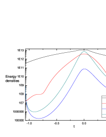
Figure 3: (Color online.) Energy densities of $\phi_{1}$, $\phi_{2}$ and $\gamma$ in the system with parameters chosen as in Fig. 1. The curves from up to down are: $\rho_{\phi_{1}}$ (black), $\rho_{\phi_{2}}$ (red), $\rho_{c}$ (dark cyan) and $\rho_{\gamma}$ (blue), respectively. The variables are also normalized with the mass scale $m_{rec}=10^{-6}m_{Pl}$.

Figs. 4, 5 and 6 give the corresponding results in the case when we choose $c>0$ while $d<0$ (with all initial conditions identical). This case seems dangerous because the contribution of the Lee-Wick scalar to the fluctuation terms could lead to an instability. However, as we have mentioned before, since the effects of the Lee-Wick scalar are less than that of the normal scalar, it is still possible for the bounce to happen. Fig. 4 shows the equation of state of the system. We can see that the evolution of $w$ is about the same as that in Fig. 1, since the change of the sign of $d$ does not alter the result too much. Fig. 5 is the behavior of scale factor in this case while Fig. 6 gives the comparison of the energy densities of all components.

Figure 4: The evolution of the equation of state $w$ as a function of cosmic time $t$ (horizontal axis). The behavior that $w$ drops to $-\infty$ indicating that a bounce takes place. The background fields are plotted in dimensionless units by normalizing by the mass $m_{rec}=10^{-6}m_{Pl}$ while the time axis is displayed in units of $m^{-1}_{rec}$. The mass parameters $m$ and $M$ were chosen to be $m=5m_{rec}$ and $M=10m_{rec}$. The initial conditions were chosen to be $\gamma_{i}\simeq-1.85\times 10^{5}m_{rec}$, $\dot{\gamma}_{i}\simeq 7.35\times 10^{6}m^{2}_{rec}$, $\phi_{1i}\simeq 1.015\times 10^{5}m_{rec}$, $\dot{\phi}_{1i}\simeq 6.39\times 10^{5}m^{2}_{rec}$, $\phi_{2i}\simeq 2.54\times 10^{2}m_{rec}$, $\dot{\phi}_{2i}\simeq-4.96\times 10^{3}m^{2}_{rec}$. The coefficients $c$ and $d$ are chosen to be $c=10^{-10}M_{rec}^{2}$ and $d=-10^{-10}M_{rec}^{2}$. The wavenumber $k\simeq 0.01hMpc^{-1}$.

Figure 5: The scale factor of the universe driven by the system with parameters chosen as in Fig. 4. From the plot we see that the bounce happens at $t=0$.

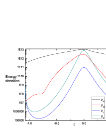
Figure 6: (Color online.) Energy densities of $\phi_{1}$, $\phi_{2}$ and $\gamma$ in the system with parameters chosen as in Fig. 4. The curves from up to down are: $\rho_{\phi_{1}}$ (black), $\rho_{\phi_{2}}$ (red), $\rho_{c}$ (dark cyan) and $\rho_{\gamma}$ (blue), respectively. The variables are also normalized with the mass scale $m_{rec}=10^{-6}m_{Pl}$.

A change in the phase of the initial radiation field velocity will not change the results (if we keep the other initial conditions fixed). On the other hand, if we flip the sign of the initial velocity of one of the two scalar fields, then the sign of the dominant contribution to the energy density as we approach the bounce will flip and this will prevent a bounce. If we use initial conditions containing two excited Fourier modes, then we obtain a bounce only if the signs of the initial field velocities are both chosen as in the first run whose results are shown here. Different phases for the scalar field velocities of the two modes destroys the possibility of obtaining a bounce.

Figures 7, 8 and 9 show the results for the equation of state parameter $w$, the Hubble parameter $H$ and the contribution of the various components to the total $\rho$ in the case of a simulation in which two Fourier modes are excited, with velocities of both scalar fields having opposite signs from those in the previous example. As is obvious, a Big Crunch singularity occurs.

Figure 7: The evolution of the equation of state $w$ as a function of cosmic time $t$ (horizontal axis). The background fields are plotted in dimensionless units by normalizing by the mass $m_{rec}=10^{-6}m_{Pl}$ while the time axis is displayed in units of $m^{-1}_{rec}$. The mass parameters $m$ and $M$ were chosen to be $m=5m_{rec}$ and $M=10m_{rec}$. This plot is the evolution of the system with two Fourier modes combined together. The one is of which the wavenumber $k\simeq 0.01hMpc^{-1}$ with initial conditions $\gamma_{i}\simeq-1.85\times 10^{5}m_{rec}$, $\dot{\gamma}_{i}\simeq 7.35\times 10^{6}m^{2}_{rec}$, $\phi_{1i}\simeq 1.015\times 10^{5}m_{rec}$, $\dot{\phi}_{1i}\simeq 6.39\times 10^{5}m^{2}_{rec}$, $\phi_{2i}\simeq 2.54\times 10^{2}m_{rec}$, $\dot{\phi}_{2i}\simeq-4.96\times 10^{3}m^{2}_{rec}$, which if taken alone will give the bounce as has been shown in the previous example. The other is of which the wavenumber $k\simeq 0.04hMpc^{-1}$ with initial conditions of the same initial values of the fields but the opposite signs of the scalar field velocity. From this plot we can see that the combination of the two Fourier mode will (generally) cause $w$ blow up, thus preventing the bounce. This means that the bounce requires special fine-tuning of the initial phases for each Fourier mode. The coefficients $c$ and $d$ are chosen to be $c=10^{-10}M_{rec}^{2}$ and $d=-10^{-10}M_{rec}^{2}$.

Figure 8: The Hubble constant of the universe driven by the system with parameters chosen as in Fig. 7. From the plot we see that there is a singularity at $t=0$.

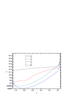
Figure 9: (Color online.) Energy densities of $\phi_{1}$, $\phi_{2}$ and $\gamma$ in the system with parameters chosen as in Fig. 7. The curves from up to down are: $\rho_{\phi_{1}}$ (black), $\rho_{\phi_{2}}$ (red), $\rho_{c}$ (dark cyan) and $\rho_{\gamma}$ (blue), respectively. The variables are also normalized with the mass scale $m_{rec}=10^{-6}m_{Pl}$.

VII Conclusions and Discussion

In this paper we analyzed in detail the possibility of obtaining a cosmological bounce in a model which corresponds to the scalar field sector of the Lee-Wick theory coupled to relativistic radiation. It is known that the scalar field sector of the Lee-Wick theory in the absence of other fields can yield a cosmological bounce Cai:2008qw . In fact, the universe will scale as non-relativistic matter with $<w>\simeq 0$ both before and after the bounce. Thus, this model is a possible realization of the “matter bounce” scenario. However, this background is unstable to the introduction of radiation since in the contracting phase the growth of energy density in radiation will exceed that of matter and will lead to a Big Crunch singularity As has been shown in previous work Karouby:2010wt , the introduction of a Lee-Wick partner to radiation does not prevent this instability. In this paper, we introduced an interaction between the radiation field and the scalar fields. The interaction could help drain energy from the radiation field to the Lee-Wick scalar, and thus could prevent the radiation from growing too fast to destroy the bounce.

We analyzed the equations describing the evolution of the three matter fields (regular scalar field, its Lee-Wick partner and the radiation field) on a cosmological background both analytically and numerically. Our analytical analysis was perturbative and made use of the second order using Born approximation. The expansion parameter is set by the initial amplitude of the gauge field. We solved the equations of motion for each field at each order, and obtained their approximations in different cases. We compared their contributions to the total energy density, and derived necessary conditions for a bounce to happen. To support our analysis, we also performed numerical calculations.

Specifically, we investigated initial conditions in which one or two Fourier modes of the radiation field and the scalar field fluctuations are excited. We found special initial conditions which indeed lead to a non-singular bounce. Changing the sign of the initial scalar field velocity will destroy the bounce solution. In the presence of two Fourier modes, we found that a bounce requires identical initial phases for the two modes. For general initial conditions, we conjecture that the measure of such initial conditions which lead to a bounce is very small. We thus find that the addition of coupling terms between the scalar fields and radiation cannot save the Lee-Wick bounce background from the instability problem with respect to the addition of radiation (nor, for that matter, with respect to scalar field fluctuations). The instability problem with respect to anisotropic stress will be even worse.

Appendix A Green’s function determination of $u_{i}^{(2)}$

The solution for the second order scalar field correction $u_{i}^{(2)}$ can be determined using the Green function method. The general solution of (103) is the sum of the solution $u_{0}(\eta)$ of the homogeneous equation which solves the same initial conditions as $u$ and the particular solution $\delta u(\eta)$ wich vanishes at time $\eta_{I}$. The particular solution is given by

$$\delta u(\eta) = u_{a}(\eta)\int_{\eta_{I}}^{\eta}d\eta^{\prime}\epsilon(\eta^{\prime})u_{b}(\eta^{\prime})s(\eta^{\prime})$$ (108)

$$-u_{b}(\eta)\int_{\eta_{I}}^{\eta}d\eta^{\prime}\epsilon(\eta^{\prime})u_{a}(\eta^{\prime})s(\eta^{\prime})~{},$$

where $u_{1}$ and $u_{2}$ are two independent solutions of the homogeneous equation, $\epsilon(\eta)$ is the Wronskian:

$$\epsilon(\eta)\,=\,\bigl{(}u_{a}^{{}^{\prime}}u_{b}-u_{b}^{{}^{\prime}}u_{a}\bigr{)}^{-1}\,,$$ (109)

and $s(\eta)$ is the source inhomogeneity.

Recall from the main text that the second order field correction terms satisfy the equations:

$$\left\{\begin{array}[]{c}{u_{1}^{(2)}}^{\prime\prime}+a^{2}m^{2}u_{1}^{(2)}=c\frac{(k^{2}\gamma^{2}-\gamma^{\prime 2})}{a^{2}}u_{1}^{(0)}~{},\\ \\ {u_{2}^{(2)}}^{\prime\prime}+a^{2}M^{2}u_{2}^{(2)}=-d\frac{(k^{2}\gamma^{2}-\gamma^{\prime 2})}{a^{2}}u_{2}^{(0)}~{},\\ \end{array}\right.$$ (113)

We will demonstrate the analysis for the case of $u_{1}^{(2)}$. Let us consider evolution for a short interval of time starting at some initial time $\eta_{I}$. Then, we can neglect the expansion of the universe in the equation of motion and take $a(\eta)=a(\eta_{I})$. We are then interested in how the result scales in $\eta_{I}$. Using this trick, the solutions of the homogeneous equation can be taken to be

$$u_{a}(\eta) = \cos(\omega_{m}\eta)$$

$$u_{b}(\eta) = \sin(\omega_{m}\eta)$$ (114)

and the Wronskian is

$$\epsilon(\eta)=-\frac{1}{\omega_{m}}\,\,\,{\rm where}\,\,\,\omega_{m}=\sqrt{a^{2}m^{2}}\,.$$ (115)

Using the result for the background $\gamma$ from the main text, the source term becomes

$$s_{\gamma}(\eta)\, = c\frac{(k^{2}\gamma^{2}-\gamma^{\prime 2})}{a^{2}}u_{1}^{(0)}$$

$$\sim a^{-2}k^{2}|\eta|^{\frac{p}{2(p-1)}}\times$$

$$\cos(2k|\eta|+2\theta_{\gamma})\cos((1-p)am|\eta|+\theta_{1}^{(0)})~{},$$

since $\gamma_{0}\sim\cos(k|\eta|+\theta_{\gamma})$.

Combining these results we obtain

$$u_{1}^{(2)} \sim -\cos(\omega_{m}\eta)\int_{\eta_{I}}^{\eta}\frac{d\eta k^{2}}{a^{3}(t)m}|\eta|^{\frac{p}{2(p-1)}}\times$$

$$\sin(\omega_{m}\eta)\cos(2k|\eta|+2\theta_{\gamma})\cos((1-p)am|\eta|+\theta_{1}^{(0)})$$

$$+\sin(\omega_{m}\eta)\int_{\eta_{I}}^{\eta}\frac{d\eta k^{2}}{a^{3}(t)m}|\eta|^{\frac{p}{2(p-1)}}\times$$

$$\cos(\omega_{m}\eta)\cos(2k|\eta|+2\theta_{\gamma})\sin((1-p)am|\eta|+\theta_{1}^{(0)})~{},$$

$$u_{2}^{(2)} \sim -\cos(\omega_{M}\eta)\int_{\eta_{I}}^{\eta}\frac{d\eta k^{2}}{a^{3}(t)M}|\eta|^{\frac{p}{2(p-1)}}\times$$

$$\sin(\omega_{M}\eta)\cos(2k|\eta|+2\theta_{\gamma})\cos((1-p)aM|\eta|+\theta_{1}^{(0)})$$

$$+\sin(\omega_{M}\eta)\int_{\eta_{I}}^{\eta}\frac{d\eta k^{2}}{a^{3}(t)M}|\eta|^{\frac{p}{2(p-1)}}\times$$

$$\cos(\omega_{M}\eta)\cos(2k|\eta|+2\theta_{\gamma})\sin((1-p)aM|\eta|+\theta_{1}^{(0)})~{}.$$

Note that if we only care about their scalings with respect to conformal time $\eta$ or scale factor $a(t)$, the above solutions can be reduced to:

$$u_{1,2}^{(2)}\propto|\eta|^{\frac{9p-2}{2(p-1)}}\propto a^{-\frac{9}{2}+\frac{1}{p}}~{},$$ (119)

and for the case of a matter dominated era where $p=2/3$, it is straightforward to show that

$$u_{1,2}^{(2)}\propto|\eta|^{-6}\propto a^{-3}~{}.$$ (120)

References

- (1) Y. F. Cai, T. t. Qiu, R. Brandenberger and X. m. Zhang, “A Nonsingular Cosmology with a Scale-Invariant Spectrum of Cosmological Perturbations from Lee-Wick Theory,” Phys. Rev. D 80 (2009) 023511 [arXiv:0810.4677 [hep-th]].
- (2) S. W. Hawking, and G. F. R. Ellis, The large scale structure of space-time, Cambridge University Press (1973); A. Borde and A. Vilenkin, Phys. Rev. Lett. 72, 3305 (1994).
- (3) A. Borde and A. Vilenkin, “Eternal Inflation And The Initial Singularity,” Phys. Rev. Lett. 72, 3305 (1994) [arXiv:gr-qc/9312022].
-
(4)
V. F. Mukhanov and R. H. Brandenberger,
“A Nonsingular universe,”
Phys. Rev. Lett. 68, 1969 (1992);
R. H. Brandenberger, V. F. Mukhanov and A. Sornborger, “A Cosmological theory without singularities,” Phys. Rev. D 48, 1629 (1993) [arXiv:gr-qc/9303001]. - (5) M. Novello and S. E. P. Bergliaffa, “Bouncing Cosmologies,” Phys. Rept. 463, 127 (2008) [arXiv:0802.1634 [astro-ph]].
- (6) D. Wands, “Duality invariance of cosmological perturbation spectra,” Phys. Rev. D 60, 023507 (1999) [arXiv:gr-qc/9809062].
- (7) F. Finelli and R. Brandenberger, “On the generation of a scale-invariant spectrum of adiabatic fluctuations in cosmological models with a contracting phase,” Phys. Rev. D 65, 103522 (2002) [arXiv:hep-th/0112249].
-
(8)
P. Peter and N. Pinto-Neto,
“Primordial perturbations in a non singular bouncing universe model,”
Phys. Rev. D 66, 063509 (2002)
[arXiv:hep-th/0203013];
F. Finelli, “Study of a class of four dimensional nonsingular cosmological bounces,” JCAP 0310, 011 (2003) [arXiv:hep-th/0307068];
L. E. Allen and D. Wands, “Cosmological perturbations through a simple bounce,” Phys. Rev. D 70, 063515 (2004) [arXiv:astro-ph/0404441];
R. Brandenberger, H. Firouzjahi and O. Saremi, “Cosmological Perturbations on a Bouncing Brane,” JCAP 0711, 028 (2007) [arXiv:0707.4181 [hep-th]];
S. Alexander, T. Biswas and R. H. Brandenberger, “On the Transfer of Adiabatic Fluctuations through a Nonsingular Cosmological Bounce,” arXiv:0707.4679 [hep-th];
F. Finelli, P. Peter and N. Pinto-Neto, “Spectra of primordial fluctuations in two-perfect-fluid regular bounces,” Phys. Rev. D 77, 103508 (2008) [arXiv:0709.3074 [gr-qc]];
A. Cardoso and D. Wands, “Generalised perturbation equations in bouncing cosmologies,” Phys. Rev. D 77, 123538 (2008) [arXiv:0801.1667 [hep-th]];
Y. F. Cai, T. Qiu, R. Brandenberger, Y. S. Piao and X. Zhang, “On Perturbations of Quintom Bounce,” JCAP 0803, 013 (2008) [arXiv:0711.2187 [hep-th]];
X. Gao, Y. Wang, W. Xue and R. Brandenberger, “Fluctuations in a Hořava-Lifshitz Bouncing Cosmology,” JCAP 1002, 020 (2010) [arXiv:0911.3196 [hep-th]];
T. Qiu and K. C. Yang, “Perturbations in Matter Bounce with Non-minimal Coupling,” JCAP 1011, 012 (2010) [arXiv:1007.2571 [astro-ph.CO]];
C. Lin, R. H. Brandenberger and L. P. Levasseur, “A Matter Bounce By Means of Ghost Condensation,” arXiv:1007.2654 [hep-th]. - (9) R. H. Brandenberger, “Inflationary cosmology: Progress and problems,” arXiv:hep-ph/9910410.
-
(10)
J. Martin and R. H. Brandenberger,
“The TransPlanckian problem of inflationary cosmology,”
Phys. Rev. D 63, 123501 (2001), [arXiv:hep-th/0005209];
R. H. Brandenberger and J. Martin, “The robustness of inflation to changes in super-Planck-scale physics,” Mod. Phys. Lett. A 16, 999 (2001) [arXiv:astro-ph/0005432]. - (11) Y. F. Cai, T. Qiu, Y. S. Piao, M. Li and X. Zhang, “Bouncing Universe with Quintom Matter,” JHEP 0710, 071 (2007) [arXiv:0704.1090 [gr-qc]].
-
(12)
T. D. Lee and G. C. Wick,
“Negative Metric and the Unitarity of the S Matrix,”
Nucl. Phys. B 9, 209 (1969);
T. D. Lee and G. C. Wick, “Finite Theory of Quantum Electrodynamics,” Phys. Rev. D 2, 1033 (1970);
B. Grinstein, D. O’Connell and M. B. Wise, “The Lee-Wick standard model,” Phys. Rev. D 77, 025012 (2008) [arXiv:0704.1845 [hep-ph]]. - (13) J. Khoury, B. A. Ovrut, P. J. Steinhardt and N. Turok, “The ekpyrotic universe: Colliding branes and the origin of the hot big bang,” Phys. Rev. D 64, 123522 (2001) [arXiv:hep-th/0103239].
- (14) J. M. Cline, S. Jeon and G. D. Moore, “The phantom menaced: Constraints on low-energy effective ghosts,” Phys. Rev. D 70, 043543 (2004) [arXiv:hep-ph/0311312].
- (15) J. Karouby and R. Brandenberger, “A Radiation Bounce from the Lee-Wick Construction?,” Phys. Rev. D 82, 063532 (2010) [arXiv:1004.4947 [hep-th]].