Least-squares fit to a straight line when each variable contains all equal errors

Abstract

The least squares fit to a straight line, when both variables are affected by all equal uncorrelated errors, leads to very simple results for both the estimated parameters and their standard errors, of widespread applicability. In this paper several formulas are derived, presenting a full set of results about the estimated parameters and their standard errors. All the results have been validated with extensive Monte Carlo simulations. The emphasis of the paper is on the calculation and properties of the best-fit parameters and their standard errors.

This paper is the expanded version of the article entitled

Linear least squares fit when both variables are affected by equal uncorrelated errors,

published in Am. J. Phys. vol. 82, 1178 (2014); http://dx.doi.org/10.1119/1.4893679.

I Introduction

Least squares fit to a straight line (LSFSL) is the subject of an extensive literature, not only in the field of physics. See, for instance, the reviews in bi:Macdonald ; bi:York and the references therein to the older literature.

A good understanding of the LSFSL is important, not only for students but also for researchers in physical sciences, because least squares fits, nowadays, are typically done by black-box computer programs. On the other hand, the availability of fast computer programs allows one to carry on long and intensive calculations and Monte Carlo simulations in a short time, often avoiding the use of approximations.

In physics, problems of LSFSL are often met such that both variables are affected by significant measurements errors, equal for all measured data points separately for both variables, and with the errors in two variables uncorrelated; this is the so-called Standard Weighting Model bi:Macdonald ; bi:PHBorcherdstAndCVShetht (SWM). In fact, the problem which triggered the work presented in this paper was the problem of reconstruction of straight line image tracks in pixelized single-photon detectors with rectangular pixels, designed for astro-particle physics experiments bi:SEUSO . Similar problems are often encountered in high-energy particle physics, when dealing with the reconstruction of particle tracks, and in the field of imaging by means of pixelized detectors. In astrophysics color-color diagrams typically lead to similar problems (see section V.1). The method proposed in this paper has been also applied in bi:Wehus . Moreover the SWM is often assumed whenever the errors of the data points are unknown and there is no reason to assume that the errors in one variable are negligible with respect to the errors in the other one. In this case the common unknown value of the error can be estimated by the fit.

The LSFSL-SWM problem can be always reduced, by a suitable rescaling of the variables, to an equivalent problem with the new dimensionless variables having equal errors bi:RBarlow . The sum of the distances between the measured data points and the best-fit straight line can thus be minimized leading to a purely geometrical problem. It is possible to solve this problem in an exact way and the results are very simple.

The purpose if this paper is to present a complete set of explicit results for the LSFSL-SWM. The results from the physics literature known to the author are quickly reviewed, and other new results are derived, including very simple analytic formulas for the standard errors of the parameters. It is shown that parameterizing the straight line with the angle with respect to one of the axes plus a second dimensional parameter leads to very simple results, having simple transformation properties under roto-translation of the Cartesian Coordinate System. It is shown that variances and covariance of the parameters can always be expressed in terms of the standard error of the angle plus purely geometrical quantities. All the results and the accuracy of the expressions for the standard errors have been cross-checked with extensive Monte Carlo simulations. The results are also compared with the results of the ordinary least squares (OLS) fit, the case of significant errors in only one of the variables, which will be called, in short bi:Macdonald , OLS-y:x fit (error on the $y$ variable only) and OLS-x:y fit (error on the $x$ variable only). A simple criterion for neglecting the error in one of the two variables is derived.

Emphasis of this paper is on the analytical, computational and practical aspects of the problem, not on its rigorous statistical treatment. All the formulas needed for a real implementation in a programming code are derived and discussed.

The outline of the paper is as follows. In section II the problem and hypotheses are presented. Results readily available in the physics literature are summarized in section III. All the new results are presented in Section IV. Section V presents a few case studies. Section VI summarizes some of the results obtained by Monte Carlo simulations carried on both to cross-check the formulas and to evaluate the accuracy of the standard errors. Finally the appendixes collect all the calculations.

II Hypotheses and the SWM

For the sake of simplicity let us introduce the symbol for the average of the generic random quantity $q$, $\langle{q}\rangle$, the symbol $\sigma[q]$ for its standard deviation and the symbol $\rho_{pq}$ for the correlation coefficient of the two random variables $p$ and $q$.

Consider a set of $N$ measured data points, described by the $\widetilde{x}$ and $\widetilde{y}$ coordinates of a suitable Cartesian Coordinate System: $\left\{\widetilde{x}_{k};\widetilde{y}_{k}\right\},(k=1,\ldots,N)$. Assume that the measured data points follow the SWM, that is: have equal standard errors, separately in both variables, $\sigma_{\widetilde{x}}\equiv\sigma[\widetilde{x}_{k}]$ and $\sigma_{\widetilde{y}}\equiv\sigma[\widetilde{y}_{k}]$, and that the errors on the $\widetilde{x}$ and $\widetilde{y}$ variables, for each measured data point, are uncorrelated:

$$\left\{\widetilde{x}_{k}\pm\sigma_{\widetilde{x}};\widetilde{y}_{k}\pm\sigma_{\widetilde{y}}\right\}\;\;\;\;\;(k=1,\ldots,N)\;\;\;\;\;\rho_{\widetilde{x}\widetilde{y}}=0\;\;\;\;\;.$$ (1)

It is assumed that each measured data point is a random sampling from a random distribution associated to each true data point, $\left\{X_{k};Y_{k}\right\}$, with true values lying on a unknown straight line, to be determined:

$$\left\{X_{k};Y_{k}\right\}\;\;\;\;\;AX_{k}+BY_{k}+C=0\;\;\;\;\;(k=1,\ldots,N)$$ (2)

$$\left\{\widetilde{x}_{k}=X_{k}+\epsilon_{\widetilde{x}};\widetilde{y}_{k}=Y_{k}+\epsilon_{\widetilde{y}}\right\}\;\;\;\;\;\text{with}\;\;\;\;\;\langle{\epsilon_{\widetilde{x}}}\rangle=0\;\;\;\;\;\sigma[\epsilon_{\widetilde{x}}]=\sigma_{\widetilde{x}}\;\;\;\;\;\langle{\epsilon_{\widetilde{y}}}\rangle=0\;\;\;\;\;\sigma[\epsilon_{\widetilde{y}}]=\sigma_{\widetilde{y}}\;\;\;\;\;,$$ (3)

where $\epsilon_{\widetilde{x}}$ and $\epsilon_{\widetilde{y}}$ are random variables, often, but not always, Gaussian random variables.

The problem can be always reduced to an equivalent problem bi:RBarlow with identical errors in both variables, by rescaling, via the standard errors, to dimensionless variables, and multiplying, for the sake of generality, by a common dimensionless factor, $\tau$:

$$\widetilde{x}_{k}\longrightarrow x_{k}\equiv\tau\left(\widetilde{x}_{k}/\sigma_{\widetilde{x}}\right)\;\;\;\;\;\Longrightarrow\;\;\;\;\;\sigma[x_{k}]=\tau\;\;\;\;\;\;\;\;\;\;\widetilde{y}_{k}\longrightarrow y_{k}\equiv\tau\left(\widetilde{y}_{k}/\sigma_{\widetilde{y}}\right)\;\;\;\;\;\Longrightarrow\;\;\;\;\;\sigma[y_{k}]=\tau\;\;\;\;\;.$$ (4)

The original variables, $\widetilde{x}_{k}$ and $\widetilde{y}_{k}$, will be called the raw variables, as opposed to the $x_{k}$ and $y_{k}$, the (re-scaled) variables. The above transformation will be always silently assumed in the rest of this paper. In every physics problem this transformation is just a change of the units of measure of the two variables, using $\sigma_{\widetilde{x}}$ and $\sigma_{\widetilde{y}}$ as the new units of measure, leading to dimensionless variables. One might choose $\tau=1$, but it is preferred to leave a generic $\tau$ in order to have a better understanding of the final formulas and deal with the case of a common but unknown error.

After the above transformation, the sum of distances between all the measured data points and the straight line, (the error function) can be minimized, as a purely geometrical problem. See bi:RBarlow for the precise probabilistic/statistical discussion.

Note that there is no point in discussing any ambiguity of the best-fit line under change of scale of the coordinates. In fact only when the errors in both variables are equal one is allowed to minimize the distance between the measured data points and the straight line, otherwise one needs to take into account the error ellipse, see for instance bi:RBarlow ; bi:Lyons .

The OLS-y:x/OLS-x:y fit can be recovered by letting $\sigma_{\widetilde{x}}\longrightarrow 0$/$\sigma_{\widetilde{y}}\longrightarrow 0$ in the final results.

Finally, let us introduce the following notations for the variance and covariance of the set of $N$ measured data points as whole, defined without the Bessel correction factor $N/\left(N-1\right)$, as it is useful in the formulation of the LSFSL problem:

$$V_{x}\equiv\langle{x^{2}}\rangle-{\langle{x}\rangle}^{2}\;\;\;\;\;V_{y}\equiv\langle{y^{2}}\rangle-{\langle{y}\rangle}^{2}\;\;\;\;\;C_{xy}\equiv\langle{xy}\rangle-\langle{x}\rangle\langle{y}\rangle\;\;\;\;\;\mathinner{\Delta\!V}\equiv V_{x}-V_{y}\;\;\;\;\;.$$ (5)

The above quantities, $V_{x}$, $V_{y}$ and $C_{xy}$, refer to the set of measured data points as a whole, describing their spatial distribution in the $xy$ plane: they are obviously distinct from the spread of one single measurement around its true value.

In order to avoid any confusion, the symbols $V_{x}$, $V_{y}$ and $C_{xy}$, are used in this paper to refer to the set of measured data points as a whole, while the symbols $\sigma_{x}^{2}$, $\sigma_{y}^{2}$ and $\rho_{xy}=0$ are used to refer to the variances and correlation coefficient of the two-dimensional random variable associated to each specific measured data point.

The relations between variances and covariance in the raw and re-scaled coordinates, necessary for taking the no-error limits, are obviously:

$$V_{x}\equiv\tau^{2}\,\cfrac{V_{\widetilde{x}}}{\sigma_{\widetilde{x}}^{2}}\,\;\;\;\;\;V_{y}\equiv\tau^{2}\,\cfrac{V_{\widetilde{y}}}{\sigma_{\widetilde{y}}^{2}}\,\;\;\;\;\;C_{xy}\equiv\tau^{2}\,\cfrac{C_{\widetilde{x}\widetilde{y}}}{\sigma_{\widetilde{x}}\sigma_{\widetilde{y}}}\,\;\;\;\;\;.$$ (6)

III The slope/intercept parametrization

The least squares fit to the straight lines

$$y=p_{y}x+q_{y}\;\;\;\;\;p_{y}=\tan[\theta_{x}]\;\;\;\;\;\text{or}\;\;\;\;\;x=p_{x}y+q_{x}\;\;\;\;\;p_{x}=\tan[\theta_{y}]\;\;\;\;\;,$$ (7)

in terms of the slopes, $p_{y}$/$p_{x}$, intercepts, $q_{y}$/$q_{x}$, and angles $\theta_{x}$/$\theta_{y}$, with respect to the $x$/$y$ axes, is appropriate in many physics problems, for instance when fitting a position as a function of time, so that the slope (velocity) can be zero but not infinity.

Some of the most well-known textbooks bi:Bevington ; bi:Cowan ; bi:Taylor ; bi:Zech ; bi:Lyons use this parametrization to describe straight lines and present the so-called effective variance method bi:Orear , to deal with measured data points having significant errors in both variables. One exception is textbook bi:RBarlow , which presents the exact solution within the SWM.

The dimensionless error function to minimize, the sum of distances between all the measured data points and the straight line, is

$$\chi^{2}_{y}[p_{y},q_{y}]\equiv\,\cfrac{1}{\tau^{2}}\,\sum_{k=1}^{N}\,\cfrac{\left(p_{y}x_{k}+q_{y}-y_{k}\right)^{2}}{1+p_{y}^{2}}\,\;\;\;\;\;\text{or}\;\;\;\;\;\chi^{2}_{x}[p_{x},q_{x}]\equiv\,\cfrac{1}{\tau^{2}}\,\sum_{k=1}^{N}\,\cfrac{\left(p_{x}y_{k}+q_{x}-x_{k}\right)^{2}}{1+p_{x}^{2}}\,\;\;\;\;\;,$$ (8)

which will be called $\chi^{2}$, regardless of its statistical properties.

Minimization of the error functions leads, after some mathematics, to the expressions for the slopes and intercepts which can be found in some of the literature bi:Ross ; bi:RBarlow ; bi:Macdonald . The solution, in both the $y$ versus $x$ and the $x$ versus $y$ representations, is:

for $$C_{xy}\neq 0 \alpha\equiv\operatorname*{\,Sign}[C_{xy}]\equiv\,\cfrac{C_{xy}}{\left|{C_{xy}}\right|}\,$$with (9)

$$A_{y}\equiv\,\cfrac{V_{y}-V_{x}}{2C_{xy}}\,\;\;\;\;\;p_{y}=A_{y}+\alpha\sqrt{1+A_{y}^{2}}=\,\cfrac{(V_{y}-V_{x})+\sqrt{4C_{xy}^{2}+\left(\mathinner{\Delta\!V}\right)^{2}}}{2C_{xy}}\,\;\;\;\;\;q_{y}=\langle{y}\rangle-p_{y}\langle{x}\rangle$$ (10)

$$A_{x}\equiv\,\cfrac{V_{x}-V_{y}}{2C_{xy}}\,\;\;\;\;\;p_{x}=A_{x}+\alpha\sqrt{1+A_{x}^{2}}=\,\cfrac{(V_{x}-V_{y})+\sqrt{4C_{xy}^{2}+\left(\mathinner{\Delta\!V}\right)^{2}}}{2C_{xy}}\,\;\;\;\;\;q_{x}=\langle{x}\rangle-p_{x}\langle{y}\rangle$$ (11)

$$\text{with $p_{y}p_{x}=1$}\;\;\;\;\;\text{and $\theta_{x}+\theta_{y}=\pi/2$}\;\;\;\;\;.$$ (12)

Note that the sign in front of the square-root is unambiguously determined by $\alpha$.

The above relation $p_{y}p_{x}=1$ is between the two different representations of the same best-fit straight line. It should not be confused with the relation between the $p_{y}$ and $p_{x}$ slopes as determined by the OLS-y:x/OLS-x:y fit, giving the correlation coefficient, $r$, of the set of data-points as whole (see for instance bi:Young ): $p_{y}p_{x}=r^{2}$.

Whenever $C_{xy}=0$ the fitted line is parallel to either the $x$ or $y$ axis. The sign of the slopes is always the same as the sign of the $C_{xy}$. The straight line perpendicular to the minimum-distance straight line maximizes the error function; its slope can be found by putting, in the above formulas, a minus sign, instead of a plus sign, in front of the square root.

A simple trigonometric transformation allows to transform equations 10 and 11 into an even simpler equation for the angles $\theta_{x}$ and $\theta_{y}$:

$$\tan[2\theta_{x}]=-\,\cfrac{1}{A_{y}}\,\;\;\;\;\;\text{for $A_{y}\neq 0$}\;\;\;\;\;\text{or}\;\;\;\;\;\tan[2\theta_{y}]=-\,\cfrac{1}{A_{x}}\,\;\;\;\;\;\text{for $A_{x}\neq 0$}\;\;\;\;\;.$$ (13)

It is useful to re-write the above equations 10 and 11 as a function of the raw variables, which also allows to take the limit of the OLS-y:x/OLS-x:y fit. One finds bi:RBarlow :

$$p_{\widetilde{y}}\equiv\tan[\theta_{\widetilde{x}}]=\,\cfrac{\sigma_{\widetilde{y}}}{\sigma_{\widetilde{x}}}\,\left(A_{y}+\alpha\sqrt{1+A_{y}^{2}}\right)\;\;\;\;\;A_{y}\equiv\,\cfrac{\sigma_{\widetilde{x}}^{2}V_{\widetilde{y}}-\sigma_{\widetilde{y}}^{2}V_{\widetilde{x}}}{2\sigma_{\widetilde{x}}\sigma_{\widetilde{y}}C_{\widetilde{x}\widetilde{y}}}\,\;\;\;\;\;,$$ (14)

$$p_{\widetilde{x}}\equiv\tan[\theta_{\widetilde{y}}]=\,\cfrac{\sigma_{\widetilde{x}}}{\sigma_{\widetilde{y}}}\,\left(A_{x}+\alpha\sqrt{1+A_{x}^{2}}\right)\;\;\;\;\;A_{x}\equiv\,\cfrac{\sigma_{\widetilde{y}}^{2}V_{\widetilde{x}}-\sigma_{\widetilde{x}}^{2}V_{\widetilde{y}}}{2\sigma_{\widetilde{x}}\sigma_{\widetilde{y}}C_{\widetilde{x}\widetilde{y}}}\,\;\;\;\;\;.$$ (15)

The standard errors on the slope and intercept will be derived in section IV.7.

IV The angle/signed-distance parametrization

IV.1 Parametrization of a straight line in the plane

In many problems the $x$ and $y$ coordinates are equivalent, such as, for instance, in straight line fitting of pixelized images with rectangular/square pixels. Especially in these case a parametrization of the straight line different from the most common slope/intercept parametrization may be useful, as the direction of the straight line is better identified by the angle with respect to one specific direction in the plane, for instance the $x$ axis, than by the slope. In fact both the slope and intercept may tend to infinity for straight lines passing near the origin and nearly parallel to the $y$ or $x$ axis (depending on the representation used from equation 7).

The details of the geometrical aspects of the parametrization of a straight line in the plane which are useful for the understanding of the results are described in this section.

Any straight line in the $xy$ plane passing by the point $\boldsymbol{R}\equiv\left\{X;Y\right\}$ can be represented in terms of the direction unit vector, $\boldsymbol{n}\equiv\left\{\cos[\theta];\sin[\theta]\right\}$, by the parametric equation

$$\boldsymbol{r}[t]=\boldsymbol{R}+\boldsymbol{n}t\;\;\;\;\;\boldsymbol{n}\equiv\left\{\cos[\theta];\sin[\theta]\right\}\;\;\;\;\;\boldsymbol{R}\equiv\left\{X;Y\right\}\;\;\;\;\;\begin{cases}x[t]=X+t\cos[\theta]\\ y[t]=Y+t\sin[\theta]\end{cases}\;\;\;\;\;.$$ (16)

Two real parameters identifying in a unique way all straight lines in the plane can be chosen as:

• the angle, $\theta$, between the straight line and the $x$ axis:

  $$-\pi/2<\theta\leq+\pi/2\;\;\;\;\;\Longrightarrow\;\;\;\;\;\cos[\theta]\geq 0\;\;\;\;\;\text{the range of $\theta$ is just one possible conventional choice}\;\;\;\;\;;$$ (17)

• the signed-distance $c$, given by the $z$ component of the vector product between $\boldsymbol{n}$ and $\boldsymbol{r}$, whose absolute value gives the distance between the straight line and the origin:

  $$-\infty<c<+\infty\;\;\;\;\;c\equiv\boldsymbol{e}_{z}\cdot\left(\boldsymbol{n}\times\boldsymbol{R}\right)\;\;\;\;\;\text{for any point $\boldsymbol{R}$ belonging to the straight line}\;\;\;\;\;;$$ (18)

  in fact the magnitude and sign of $c$ is also given by the vector product between $\boldsymbol{n}$ and the vector position of any point on the line, $\boldsymbol{R}$; the sign of $c$ is always the same as the sign of $q_{y}$.

The geometry is represented in Figure 1.

Figure 1: The angle/signed-distance parametrization.

Converting into the Cartesian representation one finds:

$$x\sin[\theta]-y\cos[\theta]+c=0$$ (19)

$$c=-X\sin[\theta]+Y\cos[\theta]\;\;\;\;\;\text{for any point $\boldsymbol{R}=\left\{X;Y\right\}$ belonging to the straight line}$$ (20)

$$\left(x-X\right)\sin[\theta]-\left(y-Y\right)\cos[\theta]=0\;\;\;\;\;.$$ (21)

Of course, other parameterizations are possible, but the above parametrization has the virtue of describing bi-univocally all straight lines in the plane in terms of two real non-singular parameters with a clear and direct geometrical interpretation. Moreover the two parameters $\theta$ and $c$ have simple transformation properties under translation and rotations in the $xy$ plane, at variance with the slope and intercept.

IV.2 Determination of the best-fit line

The error function to minimize using the angle/signed-distance parametrization is:

$$\chi^{2}[\theta,c]\equiv\,\cfrac{1}{\tau^{2}}\,\sum_{k=1}^{N}\left(x_{k}\sin[\theta]-y_{k}\cos[\theta]+c\right)^{2}\;\;\;\;\;,$$ (22)

which will be called $\chi^{2}$, regardless of its statistical properties.

Note that the problem is a non-linear least squares problem, so that the nice general properties of linear least squares problems (see for instance bi:James ) are not guaranteed. In particular the exact contour of the confidence region in the parameter space is not elliptical bi:Cowan .

All the details of the minimization of the error function in equation 22 are summarized in appendix A, where all the following results are derived.

Equating to zero the derivative with respect to $c$ of equation 22, in order to look for stationary points of the error function, immediately provides the condition that any straight line leading to a stationary point of the error function passes by the centroid of the data points, $\boldsymbol{C}\equiv\left\{\langle{x}\rangle;\langle{y}\rangle\right\}$, (as it is the case for the OLS-y:x/OLS-x:y fit):

$$\cfrac{\mathinner{\partial\chi^{2}[\theta,c]}}{\mathinner{\partial c}}=0\longrightarrow\hat{c}=-\langle{x}\rangle\sin[\hat{\theta}]+\langle{y}\rangle\cos[\hat{\theta}]\;\;\;\;\;.$$ (23)

The error function in equation 22 becomes a function of $\theta$ only, after using equation 23 to replace the signed-distance. It can be written as:

$$\,\cfrac{\tau^{2}\chi^{2}[\theta]}{N}\,\equiv\,\cfrac{1}{N}\,\sum_{k=1}^{N}\left(\left(x_{k}-\langle{x}\rangle\right)\sin[\theta]-\left(y_{k}-\langle{y}\rangle\right)\cos[\theta]\right)^{2}=V_{x}\sin^{2}[\theta]+V_{y}\cos^{2}[\theta]-2C_{xy}\sin[\theta]\cos[\theta]\;\;\;\;\;.$$ (24)

The values of $\theta$ giving the stationary points are (see appendix A for the derivation of the results) : :

$$\mathinner{\Delta\!V}=0\;\;\;\;\;\Longrightarrow\;\;\;\;\;\cos[2\theta]=0\;\;\;\;\;\Longrightarrow\;\;\;\;\;\hat{\theta}=\,\cfrac{\pi}{4}\,+q\,\cfrac{\pi}{2}\,\;\;\;\;\;q\in\mathbb{Z}$$ (25)

$$\mathinner{\Delta\!V}\neq 0\;\;\;\;\;\Longrightarrow\;\;\;\;\;\tan[2\theta]=\,\cfrac{2C_{xy}}{\mathinner{\Delta\!V}}\,\;\;\;\;\;\Longrightarrow\;\;\;\;\;\hat{\theta}=\,\cfrac{1}{2}\,\arctan[\,\cfrac{2C_{xy}}{\mathinner{\Delta\!V}}\,]+q\,\cfrac{\pi}{2}\,\;\;\;\;\;q\in\mathbb{Z}$$ (26)

$$\text{minimum: choose $\hat{\theta}$ such that $|\hat{\theta}|<\pi/2$ with the same sign as $C_{xy}$}\;\;\;\;\;.$$

In the often encountered case that the common error on the data points, $\tau$, is unknown, it can be estimated from the data. It can be shown bi:James that, in the linear least squares case, the residual sum of squares at the minimum, divided by the number of degrees of freedom, $N-2$ (as two parameters are determined by the minimization), is an unbiased estimate of the unknown error $\tau$:

$$\hat{\tau^{2}}=S^{2}\equiv\,\cfrac{\chi^{2}_{\textrm{min}}}{N-2}\,\;\;\;\;\;.$$ (27)

IV.3 Formulas for the standard errors

The simple exact analytic formulas for the standard errors and covariance of the fit parameters are presented and discussed in this section. Exact means that they can be derived without any approximation from the standard formula for the propagation of errors bi:HughesHase ; bi:RBarlow ; bi:Cowan ; bi:Zech ; bi:Lyons ; bi:James , which is derived using the first-order truncated Taylor series expansion of the function and taking expectations values. Approximate formulas were published in bi:PHBorcherdstAndCVShetht .

A long and tedious, but straightforward, direct calculation, applying the standard formula for the propagation of errors to equation 13, leads to the following results for the standard errors (see the appendix A for details of the calculation) : :

$$\boldsymbol{n}\equiv\left\{\cos[\theta];\sin[\theta]\right\}\;\;\;\;\;\boldsymbol{C}\equiv\left\{\langle{x}\rangle;\langle{y}\rangle\right\}\;\;\;\;\;Z\equiv\langle{x}\rangle\cos[\hat{\theta}]+\langle{y}\rangle\sin[\hat{\theta}]\equiv\boldsymbol{n}\cdot\boldsymbol{C}$$ (28)

$$\operatorname*{\,Var}[\hat{\theta}]\equiv\left(\mathinner{\delta\theta}\right)^{2}=\,\cfrac{\tau^{2}}{N}\,\,\cfrac{V_{x}+V_{y}}{\left(\mathinner{\Delta\!V}\right)^{2}+4C_{xy}^{2}}\,$$ (29)

$$\operatorname*{\,Var}[\hat{c}]\equiv\left(\mathinner{\delta c}\right)^{2}=\,\cfrac{\tau^{2}}{N}\,+\left(Z\mathinner{\delta\theta}\right)^{2}$$ (30)

$$\operatorname*{\,Cov}[\hat{\theta},\hat{c}]=-Z\left(\mathinner{\delta\theta}\right)^{2}\;\;\;\;\;.$$ (31)

Equations 29, 30 and 31 generalize the well-known results for the OLS-y:x/OLS-x:y fit. They can all be expressed in terms of the standard error on the angle plus the geometrical term $Z$.

$Z$ is interpreted as the signed-projection of the position vector of the centroid, $\boldsymbol{C}$, onto the direction unit vector, $\boldsymbol{n}$, of the best-fit line. The absolute value of $Z$ is the distance between the centroid and the straight line perpendicular to the best-fit line and passing by the origin.

All the above standard errors, equations 29, 30 and 31, must be invariant under rotations in the $xy$ plane as $c$ is invariant while $\theta$ is just shifted under rotations. However this property is not obvious from equations 29, 30 and 31; it is demonstrated in section IV.5.

The standard error in equation 29 must be also invariant under translations in the $xy$ plane, because $\theta$ is invariant under translations, while $c$ is not. This property is obvious from equations 29, 30 and 31, as only $Z$ is not invariant under translations in equations 29, 30 and 31.

Equation 30 shows that the error on the signed-distance $c$ is minimized if the origin of the Cartesian Coordinate System is set at the centroid of the measured data points, so that $Z=0$ (the same property applies in OLS-y:x/OLS-x:y fit). In this case the error on the signed-distance $c$ is just the expected $\tau/\sqrt{N}$, that is the error on the determination of the mean values $\langle{x}\rangle$ and $\langle{y}\rangle$, according to equation 23. Moreover if $Z=0$ the estimates of $\theta$ and $c$ are uncorrelated. In the general case equation 30 is the sum in quadrature of a term coming from the uncertainty in the position of the centroid, the first one, plus a term coming from the uncertainty in the angle, amplified by the distance $|Z|$.

It should be emphasized, as pointed out in some of the literature, that the formulas for the standard errors should be evaluated, in principle, via the true data points and not via the measured data points, as the standard error expressions are derived from a Taylor series expansion about the true data points. In practice the measured data points are normally used to evaluate the standard error expressions. The accuracy of this approximation is studied in bi:nota , via Monte Carlo simulations. In principle, after the fit, one might want to correct the measured data points to estimate the true data points values, improving the calculation of the standard errors. However it is shown in section bi:nota that this is normally not necessary.

IV.4 Bias

Since the least squares problem of Eq. 22 is a non-linear one, a possible bias of the estimates must be studied.

The bias of the estimated parameter $\hat{\theta}$ is invariant under translations and rotations of the Cartesian coordinate system, because $\theta$ itself is invariant under translations and it is just shifted by a constant under rotations. It can be shown that $\hat{\theta}$ is un-biased as follows. Imagine setting the origin of the Cartesian coordinate system at the unknown position of the centroid of the true data points, lying on the true straight line, with one axis along the true straight line, so that $\theta=0$. By symmetry, the resulting probability distributions of all the measured data points are symmetrical about the unknown true straight line. Therefore, for any configuration of measured data points, there is another configuration having all the measured data points located symmetrically with respect to the true straight line; these two symmetrical configurations, having equal probability, would give two opposite values for the estimate of $\theta$. Therefore the distribution of $\hat{\theta}$ is symmetrical about the true value, that is zero, so that the estimation of $\theta$ is un-biased.

A similar reasoning leads to a determination of the bias of the estimator $\hat{c}$ of the signed-distance. Although $c$ is invariant under rotations of the Cartesian coordinate system, its change under translations depends on the angle $\theta$. Imagine rotating the Cartesian coordinate system in such a way that the true straight line has $\theta=0$. By symmetry, the resulting probability distributions of all the measured data points are symmetrical about the unknown true straight line. Therefore, for any configuration of measured data points, there is one configuration having all the measured data points located symmetrically with respect to the true straight line. These two symmetrical configurations, having equal probability, would give: two opposite values for the estimate of $\theta$; the same value of the $x$ coordinate of the centroid of the measured data points; two different values, which average to $c$, for the $y$ coordinate of the centroid of the measured data points. Therefore, using a simple geometrical construction, one can show that the average value of the two values of $\hat{c}$ determined from these two symmetrical configurations of measured data points is $c\cos\theta$, so that the bias is:

$$\langle{\hat{c}-c}\rangle=c\langle{\cos\left(\hat{\theta}-\theta\right)}\rangle-c\;\;\;\;\;.$$ (32)

Moreover,

$$\left|{\langle{\hat{c}-c}\rangle}\right|\leq 2c\;\;\;\;\;,\;\;\;\;\;\left|{\langle{\hat{c}-c}\rangle}\right|\leq\,\cfrac{c}{2}\,\operatorname*{\,Var}\left(\hat{\theta}-\theta\right)+\mathcal{O}\left(\hat{\theta}-\theta\right)^{4}\;\;\;\;\;.$$ (33)

Using the same geometrical construction, the same result can be obtained algebraically from Eq. (23), taking into account that one has: $\hat{\theta}_{1}+\hat{\theta}_{2}=0$, $\langle{x}\rangle_{1}=\langle{x}\rangle_{2}$ and $\langle{y}\rangle_{1}+\langle{y}\rangle_{2}=2c$, for the two symmetrical configurations defined above.

IV.5 The covariance matrix and Principal Components Analysis

Principal Components Analysis (PCA) provides a better insight into the results of the LSFSL-SWM and help to derive some results in a simple way. It relies on orthogonal transformations of random variables bi:Cowan . PCA and its relation with LSFSL-SWM, discovered by K. Pearson bi:Pearson , are extensively discussed in bi:PCA .

In the rotated Cartesian Coordinate System $\left(x;y\right)\rightarrow\left(\xi;\eta\right)$, such that $\theta$ is the angle made by the $\xi$ axis with the $x$ axis, one has:

$$\xi=+x\cos[\theta]+y\sin[\theta]\;\;\;\;\;\eta=-x\sin[\theta]+y\cos[\theta]\;\;\;\;\;,$$ (34)

and the variances of the set of data points are readily calculated:

$$\begin{cases}V_{\xi}=V_{x}\cos^{2}[\theta]+V_{y}\sin^{2}[\theta]+2C_{xy}\sin[\theta]\cos[\theta]\\ V_{\eta}=V_{x}\sin^{2}[\theta]+V_{y}\cos^{2}[\theta]-2C_{xy}\sin[\theta]\cos[\theta]=V_{x}+V_{y}-V_{\xi}\;\;\;\;\;.\end{cases}$$ (35)

Therefore requiring that the variance, $V_{\eta}$, of the set of measured data points as a whole is minimized, leads to exactly the same results as minimizing equation 24. In fact the LSFSL-SWM minimizes the sum of the distances between the measured data points and the straight line at angle $\theta$ from the $x$ axis, namely the $\xi$ axis.

Equations 35 show the well-known result that the sum of the variances is invariant under rotations, as it is the trace of the covariance matrix. Therefore minimizing $V_{\eta}$ is equivalent to maximizing $V_{\xi}$. Some standard linear algebra, see for instance bi:PCA , shows that the direction $\xi$ maximizing the variance $V_{\xi}$ in equation 35 can be found by diagonalizing the covariance matrix:

$$\boldsymbol{C}\equiv\begin{pmatrix}V_{x}&C_{xy}\\ C_{xy}&V_{y}\end{pmatrix}\longrightarrow\boldsymbol{C}^{\prime}\equiv\begin{pmatrix}V_{\xi}&C_{\xi\eta}=0\\ C_{\xi\eta}=0&V_{\eta}\end{pmatrix}\;\;\;\;\;.$$ (36)

Therefore diagonalizing the covariance matrix leads to maximize the variance along the $\xi$ axis and minimize the variance along the $\eta$ axis: the largest eigenvalue, $\lambda_{+}$, is the variance along the $\xi$ axis and the smallest eigenvalue, $\lambda_{-}$, is the variance along the $\eta$ axis. The two orthonormal eigenvectors give: the direction maximizing the variance, namely the $\xi$ axis, (the eigenvector corresponding to the largest eigenvalue, $\left\{\cos[\theta];\sin[\theta]\right\}$); the direction minimizing the variance, namely the $\eta$ axis, (the eigenvector corresponding to the smallest eigenvalue), corresponding to minimize the error function in equation 22.

The following results can be obtained:

$$\lambda_{\pm}=\,\cfrac{1}{2}\,\left(\left(V_{x}+V_{y}\right)\pm\sqrt{\left(\mathinner{\Delta\!V}\right)^{2}+4C_{xy}^{2}}\right)$$ (37)

$$0\leq\lambda_{-}\leq\lambda_{+}\;\;\;\;\;\lambda_{+}+\lambda_{-}=V_{x}+V_{y}\;\;\;\;\;\lambda_{+}-\lambda_{-}=\sqrt{\left(\mathinner{\Delta\!V}\right)^{2}+4C_{xy}^{2}}\;\;\;\;\;.$$ (38)

The case of perfect linear correlation corresponds to $C_{xy}^{2}=V_{x}V_{y}$, that is zero determinant of the covariance matrix.

IV.6 Some properties of the standard errors

The discussion in section IV.5 gives some insight into the understanding of the properties of the standard errors in equations 29, 30 and 31.

The expressions for the eigenvalues of the covariance matrix, equations 37, show that the standard errors in equations 29, 30 and 31 are invariant under rotation in the $xy$ plane, as they can be written in terms of the eigenvalues of the covariance matrix and the signed-distance $Z$.

In the rotated Cartesian Coordinate System $\left(\xi;\eta\right)$, one has:

$$V_{\xi}\equiv\lambda_{+}\;\;\;\;\;V_{\eta}\equiv\lambda_{-}\;\;\;\;\;\left(\mathinner{\delta\theta}\right)^{2}=\,\cfrac{\tau^{2}}{N}\,\,\cfrac{V_{\xi}+V_{\eta}}{\left(V_{\xi}-V_{\eta}\right)^{2}}\,\;\;\;\;\;.$$ (39)

In the often encountered case that the measured data points are highly linearly correlated, the covariance can be approximately written in terms of the variances, $C_{xy}^{2}\simeq V_{x}V_{y}$, and equation 29 simplifies to:

$$\left(\mathinner{\delta\theta}\right)^{2}\simeq\,\cfrac{\tau^{2}}{N}\,\,\cfrac{1}{V_{x}+V_{y}}\,\simeq\,\cfrac{\tau^{2}}{N}\,\,\cfrac{1}{V_{\xi}}\,\;\;\;\;\;.$$ (40)

The above result for highly linearly correlated measured data points has a very simple interpretation. It shows that the standard error on the angle can be expressed as the ratio between the single data point standard error, $\tau$, and the square-root of the variance along the best-fit straight line of the set of measured data points as a whole, $\sqrt{V_{\xi}}$, divided by the square-root of the number of measured data points. Therefore the standard error on the angle can be interpreted as the transverse size of the single measured data point, $\tau$, divided by an effective length of the measured data points set, given by $\sqrt{V_{\xi}}$, similarly to the definition of the radian, all divided by the square-root of the number of measured data points.

This result can be used to easily estimate the error expected from the LSFSL-SWM, for highly linearly correlated data. Moreover it makes quantitative the naive expectation that the data points at the two extremes of the straight line have more importance for the fit, as they increase the variance $V_{\xi}$ decreasing the error on the angle. In fact: $\mathinner{\delta V_{\xi}}=2\left(\xi_{j}-\langle{\xi}\rangle\right)\mathinner{\delta\xi_{j}}/N$.

IV.7 Standard errors on the slope and intercept

Using the results derived in this section it is possible to find the formulas for the standard errors on the slope and intercept:

$$\left(\mathinner{\delta p}\right)^{2}=\left(1+p^{2}\right)^{2}\left(\mathinner{\delta\theta}\right)^{2}$$ (41)

$$\left(\mathinner{\delta q}\right)^{2}=\left(1+p^{2}\right)\left(\,\cfrac{\tau^{2}}{N}\,+\left(\mathinner{\delta\theta}\right)^{2}\left(Z-cp\right)^{2}\right)=\left(1+p^{2}\right)\left(\,\cfrac{\tau^{2}}{N}\,+\left(\mathinner{\delta\theta}\right)^{2}\langle{x}\rangle^{2}\left(1+p^{2}\right)\right)$$ (42)

$$\operatorname*{\,Cov}[p,q]=-\left(1+p^{2}\right)^{3/2}\left(Z-cp\right)\left(\mathinner{\delta\theta}\right)^{2}=-\left(1+p^{2}\right)^{2}\langle{x}\rangle\left(\mathinner{\delta\theta}\right)^{2}\;\;\;\;\;.$$ (43)

See appendix C for the details.

IV.8 Comparison with the OLS-y:x/OLS-x:y fit

The invariance under rotation of the error function (as it is a sum of distances) can be used to compare the results with the OLS-y:x/OLS-x:y fit.

The error functions in equation 8 clearly show that the results of the fit will tend to the results for the OLS-y:x/OLS-x:y fit whenever $p_{y}\simeq 0$/$p_{x}\simeq 0$, as in this case, the distance is measured in a direction which is both perpendicular to the straight line and parallel to the $y$/$x$ axis.

In fact, after determining the best-fit straight line one can apply a roto-translation to bring the origin of a new Cartesian Coordinate System, $\left\{\xi;\eta\right\}$, coincident with the centroid of the measured data points, and the $\xi$ axis along the best-fit line. In this new Cartesian Coordinate System the error function in equation 22 is exactly the same as it would be for the OLS-$\eta$:$\xi$ fit. The covariance of the set of measured data points, $C_{\xi\eta}$, is zero and the best-fit slope and intercept are both zero, in both cases by construction of the Cartesian Coordinate System $\left\{\xi;\eta\right\}$.

A more detailed discussion can be found in appendix B.

IV.9 OLS - negligible error in one of the variables

In the case of the highly linearly correlated measured data points of equation 40, it is easy to find a simple criterion to assess whenever the errors in one of the two variables can be neglected, the OLS fit.

After re-writing equation 40 in terms of the raw variables one finds:

$$\left(\mathinner{\delta\theta}\right)^{2}=\,\cfrac{\tau^{2}}{N}\,\,\cfrac{1}{V_{x}+V_{y}}\,=\,\cfrac{1}{N}\,\,\cfrac{1}{\,\cfrac{V_{\widetilde{x}}}{\sigma_{\widetilde{x}}^{2}}\,+\,\cfrac{V_{\widetilde{y}}}{\sigma_{\widetilde{y}}^{2}}\,}\,\;\;\;\;\;.$$ (44)

Note, however, that equation 44 does not give the limiting standard error on the raw angle $\widetilde{\theta}$, which is the interesting quantity, but the one on the re-scaled angle $\theta$.

The complete analysis, in the appendix B, shows that the error on $x$/$y$ is negligible depending on the relative values of $V_{\widetilde{x}}/\sigma_{\widetilde{x}}^{2}$ versus $V_{\widetilde{y}}/\sigma_{\widetilde{y}}^{2}$:

$$\begin{cases}\,\cfrac{V_{\widetilde{x}}}{\sigma_{\widetilde{x}}^{2}}\,\gg\,\cfrac{V_{\widetilde{y}}}{\sigma_{\widetilde{y}}^{2}}\,\;\;\;\;\;\Longrightarrow\;\;\;\;\;\text{\mbox{OLS-y:x}}\;\;\;\;\;\mathinner{\delta p_{\widetilde{y}}}\longrightarrow\,\cfrac{1}{\sqrt{N}}\,\,\cfrac{\sigma_{\widetilde{y}}}{\sqrt{V_{\widetilde{x}}}}\,\\ \,\cfrac{V_{\widetilde{x}}}{\sigma_{\widetilde{x}}^{2}}\,\ll\,\cfrac{V_{\widetilde{y}}}{\sigma_{\widetilde{y}}^{2}}\,\;\;\;\;\;\Longrightarrow\;\;\;\;\;\text{\mbox{OLS-x:y}}\;\;\;\;\;\mathinner{\delta p_{\widetilde{x}}}\longrightarrow\,\cfrac{1}{\sqrt{N}}\,\,\cfrac{\sigma_{\widetilde{x}}}{\sqrt{V_{\widetilde{y}}}}\,\end{cases}\;\;\;\;\;.$$ (45)

V Case studies

V.1 B. C. Reed’s example

Consider B. C. Reed’s example I bi:Reed , which was analyzed in bi:PHBorcherdstAndCVShetht by using approximate expressions for the standard errors. These data derive from a real, physical situation: calibrating the colors of globular star clusters as a function of their spectral types. The abscissa represents the difference between the ultraviolet and yellow light magnitudes of the clusters and the ordinate represents the difference between the yellow and infrared magnitudes.

The results are summarized in Figure 2 and Table 1 . The results for the LSFSL-SWM are in perfect agreement with the paper of the author while the approximate treatment of paper bi:PHBorcherdstAndCVShetht leads to slightly reduced error estimates. Note that the correlation coefficient is missing in the expressions for the standard errors, formula (10) of second paper in bi:PHBorcherdstAndCVShetht , but the authors do not use it; it is zero in the SWM. On the other hand equation (21) in the second paper in bi:Reed is correct in the commonly encountered case that the errors in the two variables are uncorrelated; unfortunately this is not explicitly stated in the text but only in end-note (9).

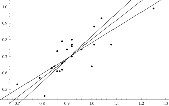
Figure 2: Data points and the three best fit lines: OLS-y:x (the smallest slope), LSFSL-SWM (the intermediate slope) and OLS-x:y (the largest slope).

OLS-y:x	$p_{y}=+0.9311\pm 0.1299$	$q_{y}=-0.1501\pm 0.1192$
OLS-x:y	$p_{y}=+1.3839\pm 0.1930$	$q_{y}=-0.5631\pm 0.1768$
LSFSL-SWM	$p_{y}=+1.1668\pm 0.1704$	$q_{y}=-0.3652\pm 0.1561$

Table 1: Best fit results (slope, intercept): OLS-y:x, LSFSL-SWM and OLS-x:y.

Since the data are given with only two significant figures, the number of digits quoted is not justified. However, following B. C. Reed bi:Reed , the point is to provide figures against which others can compare the results of their own algorithms as if the original data are regarded as exact.

The results of PCA are shown in Figure 3.

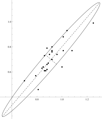
Figure 3: Data points and results of PCA: the ellipse has its semi-axes along the directions of the eigenvectors and the semi-axes have the same length as the eigenvalues.

V.2 A light-detector

Consider a CCD-like light detector, where the image produced by a suitable optics is focused (a camera, for instance). Suppose it must be used to identify straight light tracks, produced by a moving point-like light source in the night sky, for instance to observe meteors, airplanes or extensive air-showers produced by cosmic radiation bi:SEUSO . Let the typical length of the track be $\sigma_{L}$, defined as the standard deviation of the data points along the track.

Assume, firstly, that the combination of the intrinsic spread of the point-like light source and the point-spread function of the optics gives, on the photo-detector plane, a standard deviation $\sigma_{x}=\sigma_{y}\equiv\tau$ much larger than the pixel size, so that binning effects can be neglected. The expected angular resolution can be estimated as (equation 40):

$$\mathinner{\delta\theta}\simeq\,\cfrac{\tau}{\sqrt{N}}\,\,\cfrac{1}{\sqrt{V_{\xi}}}\,=\,\cfrac{\tau}{\sqrt{N}}\,\,\cfrac{1}{\sigma_{L}}\,\;\;\;\;\;.$$ (46)

As a second example consider the case that the pixel size, $d$, is much larger than the transverse size of the image track on the photo-detector plane. The uncertainty on the measurements can be taken as $\tau=d/\sqrt{12}$, assuming a uniform probability distribution inside the pixel. Assuming uncorrelated measurements, the expected angular resolution can be estimated as (equation 40):

$$\mathinner{\delta\theta}\simeq\,\cfrac{\tau}{\sqrt{N}}\,\,\cfrac{1}{\sqrt{V_{\xi}}}\,=\,\cfrac{1}{\sqrt{N}}\,\,\cfrac{d}{\sqrt{12}}\,\,\cfrac{1}{\sigma_{L}}\,\;\;\;\;\;.$$ (47)

Both analytical relations can be used to optimize the photo-detector parameters, given the desired angular resolution.

V.3 Kinematics of a image track in a photo-detector

The explicit analytical formula 29 was used, in reference bi:SEUSO , in the design of a photo-detector to observe the image track of the extensive air-showers produced in the atmosphere by ultra high energy cosmic radiation. The explicit analytical formulas, written in terms of the photo-detector parameters, were then used to optimize the photo-detector design.

VI Toy Monte Carlo simulations

VI.1 Setup of the toy Monte Carlo simulations

In order to cross-check and evaluate the accuracy of the formulas for the standard errors derived in this paper, extensive Monte Carlo simulations bi:Wolfram were carried on as follows.

1. Straight lines were simulated in the $xy$ plane, with uniformly distributed random angle $\theta$ and a Gaussian distribution of the signed-distance, $c$, with zero mean and a standard deviation of $D=1$. For each straight line a fixed number, $N$, of true data points was simulated, on the straight line, with a uniform random distribution along a segment of length $L=1$ of the straight line.

2. Each true data point was converted into a simulated measured data point (i.e. simulated measurements) according to a bi-dimensional Gaussian distribution centered at the true data point and having equal fixed standard errors, $\tau\equiv\sigma_{x}=\sigma_{y}$, and zero correlation coefficient. The best-fit straight line was then calculated.

3. For each simulated straight line and its set of true data points, the procedure at step 2) was repeated for a number of times; each repetition is called one iteration and, typically, the number of iterations is $n_{I}\approx 1000$. Statistics was then collected of the fitted angle/signed-distance results, for one specific true straight line and its set of true data points.

4. The procedure at steps 1), 2) and 3) was repeated by simulating a number of different straight lines; each simulation of one straight line is called one run and, typically, the number of runs is $n_{R}\approx 1000$. For all the runs, statistics was collected of the fitted parameters with respect to the known true parameters of the simulated straight line and its set of true data points.

5. The procedure at steps 1), 2), 3) and 4) was then repeated for different values of the number of measured data points, $N$, and of the standard error of the single data point, $\tau$. The different values for $N$ and $\tau$ where chosen in such a way to keep an approximately constant ratio between one value and the next one, inside a pre-defined fixed range. Therefore different sets of parameters, $\left(N,\tau\right)$, were simulated, with: $3\leq N\leq 100$ and $0.001\leq\tau\leq 1$, as follows:

   $$N=\left\{3;4;5;6;8;10;15;20;30;50;100\right\};$$ (48)

   $$\tau:\begin{cases}\;\;\;\;\;\text{coarse-scan in $\tau$:}\;\;\;\;\;\tau=\left\{1;0.1;0.01;0.001\right\}\propto 10^{-k}\\ \;\;\;\;\;\text{fine-scan in $\tau$:}\;\;\;\;\;\tau=\left\{0.1;0.0631;0.0398;0.0251;0.0158;0.01\right\}\propto 10^{-k/5}\end{cases}$$ (49)

The problem is invariant under a common rescaling of the two coordinates, so that the results are expected to depend only on the ratio $\tau/L$.

The largest simulated value of the data point error, $\tau/L=1$, would give so large errors with respect to the length of the segment of the straight line that it is a non realistic case. It has been simulated to verify that, in this case, the approximation of the standard formula for the propagation of errors fails and to determine under what conditions the formula becomes an accurate estimate of the standard error.

It would be also possible to simulate straight lines with absolute values of the signed distance, $c\gtrsim L=1$. However the standard error formulas, equations 29, 30 and 31, show that it is better to set the origin of the Cartesian Coordinate System as close as possible to the centroid of the measured data points, in order to have $c\simeq 0$, so that $Z\simeq 0$ and both the error on the signed distance and the covariance between the angle and the signed-distance are minimized. This is of course always possible, by means of a suitable translation, and therefore there is no need to simulate larger absolute values of the signed-distance.

For both the angle $\theta$ and the signed-distance $c$, the three following quantities were calculated.

1. The standard deviation of the distributions of the fitted angle and signed-distance, $\hat{\sigma}[\hat{\theta}]$ and $\hat{\sigma}[\hat{c}]$, were calculated for every run; for any set of parameters the average was taken over all the runs: $\langle{\hat{\sigma}[\hat{\theta}]}\rangle$ and $\langle{\hat{\sigma}[\hat{c}]}\rangle$.

   This is what is usually defined as the standard deviation of the estimator.

2. Equations 29 and 30 were used, for all iterations of every run, to calculate the standard errors from the simulated measured data points (i.e. simulated measurements) and the median was taken over all iterations of every run, $M[\hat{\mathinner{\delta\theta}}]$ and $M[\hat{\mathinner{\delta c}}]$; for any set of parameters the average was taken over all the runs: $\langle{M[\hat{\mathinner{\delta\theta}}]}\rangle$ and $\langle{M[\hat{\mathinner{\delta c}}]}\rangle$.

   This is an estimate of the typical error one would calculate from a real set of data points. The median is used in order to provide a robust estimation, as outlying large values may show-up for certain combinations of true data-points (for instance all true data-points clustered one close to the other).

3. For each run the standard errors were computed from the true data points via equations 29, for $\mathinner{\delta\theta}_{0}$, and 30, for $\mathinner{\delta c}_{0}$; for any set of parameters the average was taken over all the runs: $\langle{\mathinner{\delta\theta}_{0}}\rangle$ and $\langle{\mathinner{\delta c}_{0}}\rangle$.

   For any given straight line and any set of true data-points on it, $\mathinner{\delta\theta}_{0}$ and $\mathinner{\delta c}_{0}$ are the expected standard errors calculated by the standard formula for the propagation of errors. Therefore $\langle{\mathinner{\delta\theta}_{0}}\rangle$ and $\langle{\mathinner{\delta c}_{0}}\rangle$ are a sort of reference values, setting the expected magnitude of the standard errors, for any given set of parameters, and useful as normalization factors to compare different set of parameters.

Some of the results obtained by the extensive Monte Carlo simulations are summarized in the rest of this section.

VI.2 Results of the toy Monte Carlo simulations

The results of the different simulations were re-normalized by $\tau$, in order to compare results for different values of $\tau$, and are shown as a function of $N$ for different values of $\tau/L$.

VI.2.1 Results for $\langle{\mathinner{\delta\theta}_{0}}\rangle$ and $\langle{\mathinner{\delta c}_{0}}\rangle$

All the simulations for $\langle{\mathinner{\delta\theta}_{0}}\rangle$ and $\langle{\mathinner{\delta c}_{0}}\rangle$, after normalizing for $\tau$, show a very similar behavior as a function of $N$, for the different values of $\tau/L$, as shown in Figure 4.

The behavior as a function of $N$ is fitted by $\sim 1/\sqrt{N+4}$, for $\langle{\mathinner{\delta\theta}_{0}}\rangle$, and by $\sim 1/\sqrt{N+1}$, for $\langle{\mathinner{\delta c}_{0}}\rangle$ (the result of the fit not shown in the Figures).

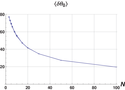
(a) Angle $\theta$.

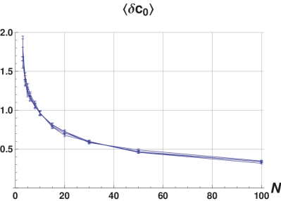
(b) Signed-distance $c$.

Figure 4: Results of the simulations for $\langle{\mathinner{\delta\theta}_{0}}\rangle$ and $\langle{\mathinner{\delta c}_{0}}\rangle$, as a function of $N$, for $\tau/L=\left\{1;0.1;0.01;0.001\right\}$. The four curves on each plot are well superimposed and barely distinguishable. Errors bars are very small and barely visible as well.

VI.2.2 Results for $\langle{\hat{\sigma}[\hat{\theta}]}\rangle$ and $\langle{\hat{\sigma}[\hat{c}]}\rangle$

All the simulations for $\langle{\hat{\sigma}[\hat{\theta}]}\rangle$ and $\langle{\hat{\sigma}[\hat{c}]}\rangle$, after normalizing for $\tau$, show a very similar behavior as a function of $N$, for the different values of $\tau/L\lesssim 0.05$, as shown individually in Figure 5 and all together in Figure 6.

Moreover, for values $\tau/L\lesssim 0.05$, the behavior as a function of $N$ is fitted by $\sim 1/\sqrt{N+4}$, for $\langle{\hat{\sigma}[\hat{\theta}]}\rangle$, and by $\sim 1/\sqrt{N+1}$, for $\langle{\hat{\sigma}[\hat{c}]}\rangle$ (the result of the fit not shown in the Figures).

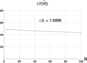
(a) Angle $\theta$.

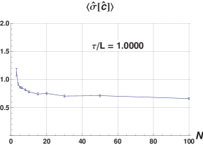
(b) Signed-distance $c$.

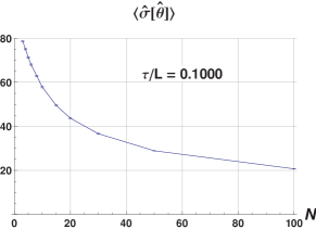
(c) Angle $\theta$.

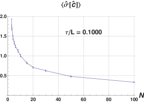
(d) Signed-distance $c$.

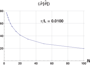
(e) Angle $\theta$.

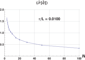
(f) Signed-distance $c$.

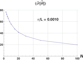
(g) Angle $\theta$.

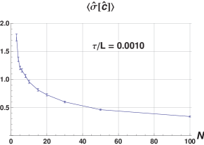
(h) Signed-distance $c$.

Figure 5: Results of the simulations for $\langle{\hat{\sigma}[\hat{\theta}]}\rangle$ and $\langle{\hat{\sigma}[\hat{c}]}\rangle$, as a function of $N$, for $\tau/L=\left\{1;0.1;0.01;0.001\right\}$. Errors bars are very small and barely visible.

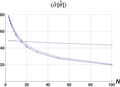
(a) Angle $\theta$.

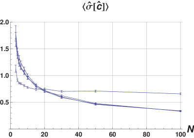
(b) Signed-distance $c$.

Figure 6: Results of the simulations for $\langle{\hat{\sigma}[\hat{\theta}]}\rangle$ and $\langle{\hat{\sigma}[\hat{c}]}\rangle$, as a function of $N$, for $\tau/L=\left\{1;0.1;0.01;0.001\right\}$. The two almost horizontal curves on each plot correspond to $\tau/L=1$. The two curves with the smallest $\tau/L$ are well superimposed and barely distinguishable. Errors bars are very small and barely visible.

In order to study the behavior for $0.01\lesssim\tau/L\lesssim 0.1$, a finer scan has been done in this interval; the plots are individually shown in Figure 7, for $\tau/L=\left\{0.0631;0.0398;0.0251;0.0158\right\}$, and all together in Figure 8, for $\tau/L=\left\{0.1;0.0631;0.0398;0.0251;0.0158;0.01\right\}$.

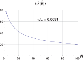
(a) Angle $\theta$.

(b) Signed-distance $c$.

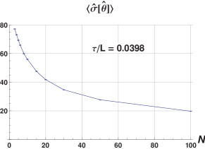
(c) Angle $\theta$.

(d) Signed-distance $c$.

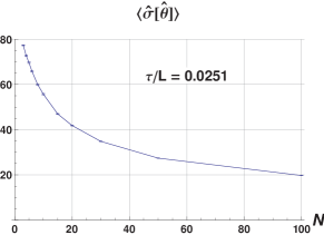
(e) Angle $\theta$.

(f) Signed-distance $c$.

(g) Angle $\theta$.

(h) Signed-distance $c$.

Figure 7: Results of the simulations for $\langle{\hat{\sigma}[\hat{\theta}]}\rangle$ and $\langle{\hat{\sigma}[\hat{c}]}\rangle$, as a function of $N$, for $\tau/L=\left\{0.0631;0.0398;0.0251;0.0158\right\}$. Errors bars are very small and barely visible.

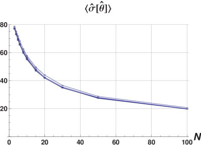
(a) Angle $\theta$.

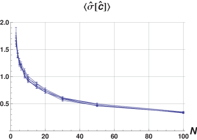
(b) Signed-distance $c$.

Figure 8: Results of the simulations for $\langle{\hat{\sigma}[\hat{\theta}]}\rangle$ and $\langle{\hat{\sigma}[\hat{c}]}\rangle$, as a function of $N$, for $\tau/L=\left\{0.1;0.0631;0.0398;0.0251;0.0158;0.01\right\}$. Errors bars are very small and barely visible.

Afterward, in order to get rid of the variability associated with the random straight line and random set of true data-points on the straight line, the values of $\langle{\hat{\sigma}[\hat{\theta}]}\rangle$ and $\langle{\hat{\sigma}[\hat{c}]}\rangle$ were normalized to $\langle{\mathinner{\delta\theta}_{0}}\rangle$ and $\langle{\mathinner{\delta c}_{0}}\rangle$.

For $\tau\lesssim 0.02$, no statistically significant difference with $\langle{\mathinner{\delta\theta}_{0}}\rangle$ and $\langle{\mathinner{\delta c}_{0}}\rangle$ has been found and the ratios $\langle{\hat{\sigma}[\hat{\theta}]}\rangle/\langle{\mathinner{\delta\theta}_{0}}\rangle$ and $\langle{\hat{\sigma}[\hat{c}]}\rangle/\langle{\mathinner{\delta c}_{0}}\rangle$ are compatible with one, as shown in Figure 9.

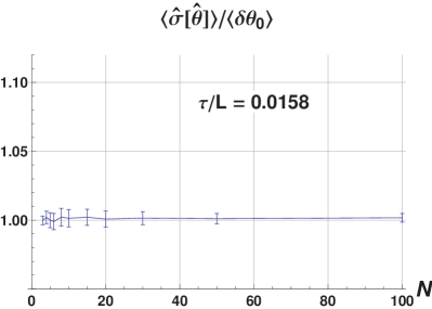
(a) Angle $\theta$.

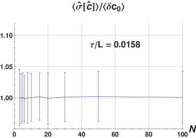
(b) Signed-distance $c$.

Figure 9: Results of the simulations for the ratios $\langle{\hat{\sigma}[\hat{\theta}]}\rangle/\langle{\mathinner{\delta\theta}_{0}}\rangle$ and $\langle{\hat{\sigma}[\hat{c}]}\rangle/\langle{\mathinner{\delta c}_{0}}\rangle$, as a function of $N$, for $\tau/L=0.0158$.

On the other hand the behavior of the ratios $\langle{\hat{\sigma}[\hat{\theta}]}\rangle/\langle{\mathinner{\delta\theta}_{0}}\rangle$ and $\langle{\hat{\sigma}[\hat{c}]}\rangle/\langle{\mathinner{\delta c}_{0}}\rangle$ for values of $\tau/L\gtrsim 0.02$, as shown in Figure 10, shows a significant departure from the expected $\langle{\mathinner{\delta\theta}_{0}}\rangle$ and $\langle{\mathinner{\delta c}_{0}}\rangle$, but not larger than $\approx 5\%$ for $\tau\lesssim 0.1$.

As a general trend, the ratios tend to one as $\tau/L$ decreases, as expected thanks to the improvement of the approximations made to derive the standard formula for the propagation of errors. Moreover the ratios tend to one at small $N$ anyway because at small $N$ the values of the numerator and denominator became large with respect to their difference.

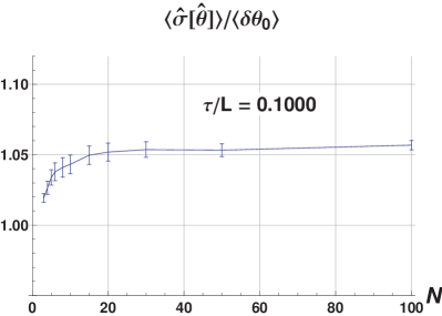
(a) Angle $\theta$.

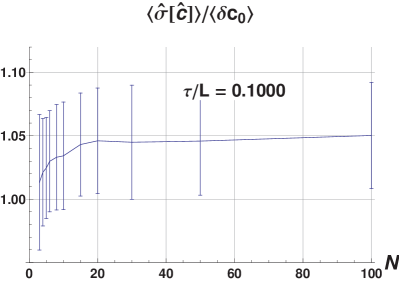
(b) Signed-distance $c$.

Figure 10: Results of the simulations for the ratios $\langle{\hat{\sigma}[\hat{\theta}]}\rangle/\langle{\mathinner{\delta\theta}_{0}}\rangle$ and $\langle{\hat{\sigma}[\hat{c}]}\rangle/\langle{\mathinner{\delta c}_{0}}\rangle$, as a function of $N$, for $\tau/L=0.1$.

VI.2.3 Results for $\langle{M[\hat{\mathinner{\delta\theta}}]}\rangle$ and $\langle{M[\hat{\mathinner{\delta c}}]}\rangle$

All the simulations for $\langle{M[\hat{\mathinner{\delta\theta}}]}\rangle$ and $\langle{M[\hat{\mathinner{\delta c}}]}\rangle$, after normalizing for $\tau$, show a very similar behavior as a function of $N$, for the different values of $\tau/L\lesssim 0.05$, as shown individually in Figure 11 and all together in Figure 12.

Moreover, for values $\tau/L\lesssim 0.05$, the behavior as a function of $N$ is fitted by $\sim 1/\sqrt{N+4}$, for $\langle{M[\hat{\mathinner{\delta\theta}}]}\rangle$, and by $\sim 1/\sqrt{N+1}$, for $\langle{M[\hat{\mathinner{\delta c}}]}\rangle$ (the result of the fit not shown in the Figures).

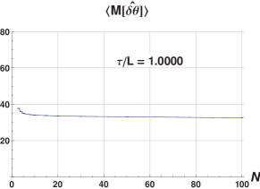
(a) Angle $\theta$.

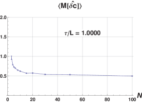
(b) Signed-distance $c$.

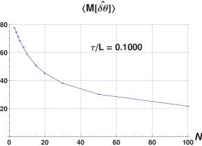
(c) Angle $\theta$.

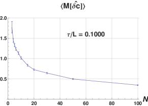
(d) Signed-distance $c$.

(e) Angle $\theta$.

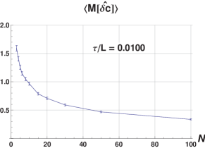
(f) Signed-distance $c$.

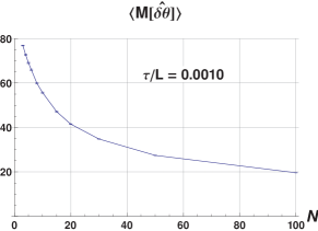
(g) Angle $\theta$.

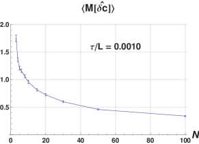
(h) Signed-distance $c$.

Figure 11: Results of the simulations for $\langle{M[\hat{\mathinner{\delta\theta}}]}\rangle$ and $\langle{M[\hat{\mathinner{\delta c}}]}\rangle$, as a function of $N$, for $\tau/L=\left\{1;0.1;0.01;0.001\right\}$. Errors bars are very small and barely visible.

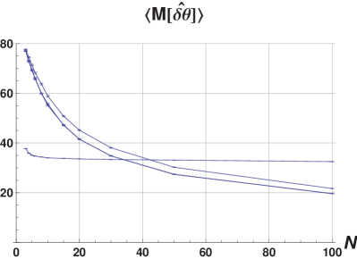
(a) Angle $\theta$.

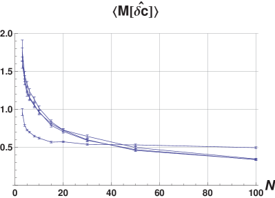
(b) Signed-distance $c$.

Figure 12: Results of the simulations for $\langle{M[\hat{\mathinner{\delta\theta}}]}\rangle$ and $\langle{M[\hat{\mathinner{\delta c}}]}\rangle$, as a function of $N$, for $\tau/L=\left\{1;0.1;0.01;0.001\right\}$. The two almost horizontal curves on each plot correspond to $\tau/L=1$. The two curves with the smallest $\tau/L$ are well superimposed and barely distinguishable. Errors bars are very small and barely visible.

In order to study the behavior for $0.01\lesssim\tau/L\lesssim 0.1$, a finer scan has been done in this interval; the plots are individually shown in Figure 13, for $\tau/L=\left\{0.0631;0.0398;0.0251;0.0158\right\}$, and all together in Figure 14, for $\tau/L=\left\{0.1;0.0631;0.0398;0.0251;0.0158;0.01\right\}$.

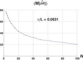
(a) Angle $\theta$.

(b) Signed-distance $c$.

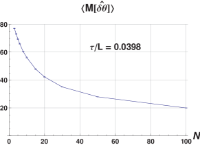
(c) Angle $\theta$.

(d) Signed-distance $c$.

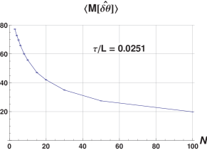
(e) Angle $\theta$.

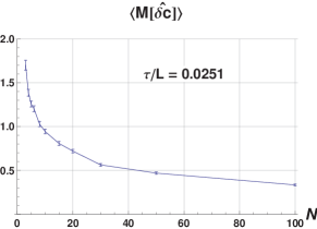
(f) Signed-distance $c$.

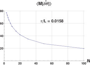
(g) Angle $\theta$.

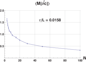
(h) Signed-distance $c$.

Figure 13: Results of the simulations for $\langle{M[\hat{\mathinner{\delta\theta}}]}\rangle$ and $\langle{M[\hat{\mathinner{\delta c}}]}\rangle$, as a function of $N$, for $\tau/L=\left\{0.0631;0.0398;0.0251;0.0158\right\}$.

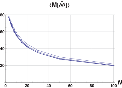
(a) Angle $\theta$.

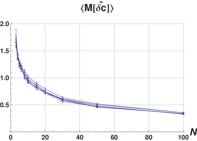
(b) Signed-distance $c$.

Figure 14: Results of the simulations for $\langle{M[\hat{\mathinner{\delta\theta}}]}\rangle$ and $\langle{M[\hat{\mathinner{\delta c}}]}\rangle$, as a function of $N$, for $\tau/L=\left\{0.1;0.0631;0.0398;0.0251;0.0158;0.01\right\}$. Errors bars are very small and barely visible.

Afterward, in order to get rid of the variability associated with the random straight line and random set of true data-points on the straight line, the values of $\langle{M[\hat{\mathinner{\delta\theta}}]}\rangle$ and $\langle{M[\hat{\mathinner{\delta c}}]}\rangle$ were normalized to $\langle{\mathinner{\delta\theta}_{0}}\rangle$ and $\langle{\mathinner{\delta c}_{0}}\rangle$.

For $\tau\lesssim 0.02$, no statistically significant difference with $\langle{\mathinner{\delta\theta}_{0}}\rangle$ and $\langle{\mathinner{\delta c}_{0}}\rangle$ has been found and the ratios $\langle{M[\hat{\mathinner{\delta\theta}}]}\rangle/\langle{\mathinner{\delta\theta}_{0}}\rangle$ and $\langle{M[\hat{\mathinner{\delta c}}]}\rangle/\langle{\mathinner{\delta c}_{0}}\rangle$ are compatible with one, as shown in Figure 15.

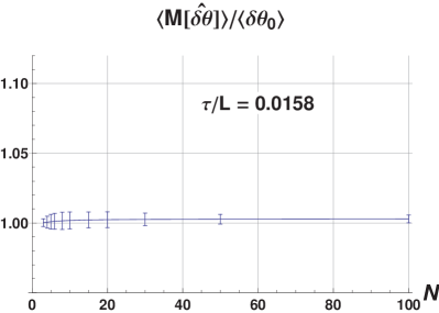
(a) Angle $\theta$.

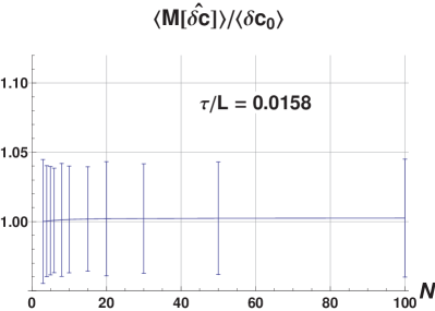
(b) Signed-distance $c$.

Figure 15: Results of the simulations for the ratios $\langle{M[\hat{\mathinner{\delta\theta}}]}\rangle/\langle{\mathinner{\delta\theta}_{0}}\rangle$ and $\langle{M[\hat{\mathinner{\delta c}}]}\rangle/\langle{\mathinner{\delta c}_{0}}\rangle$, as a function of $N$, for $\tau/L=0.0158$.

On the other hand the behavior of the ratios $\langle{M[\hat{\mathinner{\delta\theta}}]}\rangle/\langle{\mathinner{\delta\theta}_{0}}\rangle$ and $\langle{M[\hat{\mathinner{\delta c}}]}\rangle/\langle{\mathinner{\delta c}_{0}}\rangle$ for values of $\tau/L\gtrsim 0.02$, as shown in Figure 16, shows a significant departure from the expected $\langle{\mathinner{\delta\theta}_{0}}\rangle$ and $\langle{\mathinner{\delta c}_{0}}\rangle$, but not larger than $\approx 10\%$ for $\tau\lesssim 0.1$.

As a general trend, the ratios tend to one as $\tau/L$ decreases, as expected thanks to the improvement of the approximations made to derive the standard formula for the propagation of errors. Moreover the ratios tend to one at small $N$ anyway because at small $N$ the values of the numerator and denominator became large with respect to their difference.

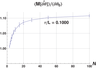
(a) Angle $\theta$.

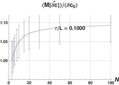
(b) Signed-distance $c$.

Figure 16: Results of the simulations for the ratios $\langle{M[\hat{\mathinner{\delta\theta}}]}\rangle/\langle{\mathinner{\delta\theta}_{0}}\rangle$ and $\langle{M[\hat{\mathinner{\delta c}}]}\rangle/\langle{\mathinner{\delta c}_{0}}\rangle$, as a function of $N$, for $\tau/L=0.1$.

VI.3 Conclusions from the Monte Carlo simulations

The main results of the Monte Carlo simulations presented in the previous sections can be summarized as follows.

• The standard errors, equations 29 and 30, calculated from the true data points, $\langle{\mathinner{\delta(.)}_{0}}\rangle$, scale as $\sim 1/\sqrt{N+4}$, for $\theta$, and as $\sim 1/\sqrt{N+1}$, for $c$, at fixed $\tau/L$. Normalization by $\tau$ provides, for $\tau/L\lesssim 0.02$, a universal curve as a function of $N$.

• Both the standard deviation of the estimators of the parameters, $\theta$ and $c$, $\langle{\hat{\sigma}[\hat{(.)}]}\rangle$, and the standard errors, equations 29 and 30, calculated from the measured data points, $\langle{M[\hat{\mathinner{\delta(.)}}]}\rangle$, as long as $\tau/L\lesssim 0.05$, scale, at fixed $\tau/L$, as $\sim 1/\sqrt{N+4}$, for $\theta$, and as $\sim 1/\sqrt{N+1}$, for $c$. Normalization by $\tau$ provides, for $\tau/L\lesssim 0.02$, a universal curve as a function of $N$.

• The standard errors, equations 29 and 30, calculated from the measured data points, $\langle{M[\hat{\mathinner{\delta\theta}}]}\rangle$ and $\langle{M[\hat{\mathinner{\delta c}}]}\rangle$, are reliable estimates of the standard deviation of the estimators of $\theta$ and $c$, $\langle{\hat{\sigma}[\hat{(.)}]}\rangle$, to within $\approx 10\%$ for $\tau/L\lesssim 0.1$. In particular, to within $\approx 10\%$, it shall not be necessary to re-evaluate the standard errors using the estimated true data points values after the best-fit straight line has been determined.

• For $\tau/L\lesssim 0.02$, the standard errors, equations 29 and 30, both calculated from the true data points, $\langle{\mathinner{\delta(.)}_{0}}\rangle$, and calculated from the measured data points, $\langle{M[\hat{\mathinner{\delta(.)}}]}\rangle$, and the standard deviation of the estimators of the parameters, $\langle{\hat{\sigma}[\hat{(.)}]}\rangle$, do not show any difference, within the statistical uncertainty of the Monte Carlo simulations.

The following additional conclusions were obtained by the Monte Carlo simulations, and stated without showing explicit evidence in this paper.

• Lack of bias of the two estimators, to within the statistical uncertainty.

• Excellent normality of the distribution of the $\hat{\theta}$ estimator, for all the simulated parameters, to within the statistical uncertainty, according to common statistical tests, such as Cramér-von Mises and Kolmogorov-Smirnov bi:James .

• Excellent normality of the distribution of the $\hat{c}$ estimator, whenever $\tau/L\lesssim 0.01$, to within the statistical uncertainty. For larger values of $\tau/L$ strong deviations from normality start to be very significant for small values of $N$ and less significant for large values of $N$; for instance, Cramér-von Mises and Kolmogorov-Smirnov tests give a P-value less than $\approx 0.001$ whenever $\tau/L=0.1$ and $N\lesssim 37$. The distributions, deviating from a Gaussian shape, show a positive excess kurtosis.

VII Conclusions

Simple formulas for both the best-fit parameters and their standard errors in the LSFSL-SWM have been derived, using the angle/signed-distance parametrization of the straight line, and validated with Monte Carlo simulations.

Several properties of the standard errors were derived and investigated. The standard errors in the slope/intercept parameterization were derived. A simple relation for the case of highly-correlated measurements was derived. The extent to which errors in one of the variables can be neglected is quantified and the limiting case of the OLS-y:x/OLS-x:y fit was studied.

Appendix A Derivation of the best-fit line

The search for stationary points of the error function in equation 22 (including the minimum point) leads to the two equations:

$$\left(\mathinner{\Delta\!V}\right)\sin[2\theta]-2C_{xy}\cos[2\theta]=0$$ (50)

$$\langle{x}\rangle\sin[\theta]-\langle{y}\rangle\cos[\theta]+c=0\;\;\;\;\;.$$ (51)

The solution of equation 50 uses standard and well-known trigonometric procedures. However some care is required for the proper handling of the trigonometric functions. After the angle $\theta$ is found, equation 51 allows to determine $c$ in a trivial way.

Equation 50 always has two distinct solutions for $2\theta$, differing by $\pm\pi$, in the interval $0\leq 2\theta<2\pi$, as it is well-known from elementary trigonometry. In fact, letting $X=\cos[2\theta]$ and $Y=\sin[2\theta]$ and using $X^{2}+Y^{2}=1$ the interpretation of the equation in terms of analytic geometry immediately leads to the conclusion.

Therefore there are four distinct solutions for $\theta$, in the interval $0\leq 2\theta<2\pi$, differing by $\pm\pi/2$. Two of them, differing by $\pm\pi$, minimize the error function and corresponds to the same straight line. The other two solutions, orthogonal to the first ones, maximize the error function.

First note that the sign of the product $\mathinner{\Delta\!V}C_{xy}$ is the same as the sign of the product $\sin[2\theta]\cos[2\theta]$, so that this determines in which quadrant the angle $2\theta$ lies:

$$\mathinner{\Delta\!V}C_{xy}\lessgtr 0\;\;\;\;\;\Longleftrightarrow\;\;\;\;\;\sin[2\theta]\cos[2\theta]\lessgtr 0\;\;\;\;\;.$$ (52)

Second, the following special cases arise:

$$\mathinner{\Delta\!V}=0\;\;\;\;\;\Longleftrightarrow\;\;\;\;\;\cos[2\theta]=0\;\;\;\;\;\Longleftrightarrow\;\;\;\;\;\theta=\,\cfrac{\pi}{4}\,+q\,\cfrac{\pi}{2}\,\;\;\;\;\;q\in\mathbb{Z}$$ (53)

$$C_{xy}=0\;\;\;\;\;\Longleftrightarrow\;\;\;\;\;\sin[2\theta]=0\;\;\;\;\;\Longleftrightarrow\;\;\;\;\;\theta=q\,\cfrac{\pi}{2}\,\;\;\;\;\;q\in\mathbb{Z}\;\;\;\;\;.$$ (54)

Finally, if $\mathinner{\Delta\!V}\neq 0$ equation 50 can be safely reduced to:

$$\mathinner{\Delta\!V}\neq 0\;\;\;\;\;\Longleftrightarrow\;\;\;\;\;\tan[2\theta]=\,\cfrac{2C_{xy}}{\mathinner{\Delta\!V}}\,\;\;\;\;\;\theta=\,\cfrac{1}{2}\,\arctan[\,\cfrac{2C_{xy}}{\mathinner{\Delta\!V}}\,]+q\,\cfrac{\pi}{2}\,\;\;\;\;\;q\in\mathbb{Z}\;\;\;\;\;.$$ (55)

Equation 55 for $\theta$ provides two angles in the range $-\pi/2<\theta<+\pi/2$, differing by $\pi/2$, one corresponding to a minimum and the other to a maximum of the error function.

Equation 55 immediately implies the useful relations:

$$\cos^{2}[2\theta]=\,\cfrac{\left(\mathinner{\Delta\!V}\right)^{2}}{\left(\mathinner{\Delta\!V}\right)^{2}+4C_{xy}^{2}}\,\;\;\;\;\;\sin^{2}[2\theta]=\,\cfrac{4C_{xy}^{2}}{\left(\mathinner{\Delta\!V}\right)^{2}+4C_{xy}^{2}}\,\;\;\;\;\;.$$ (56)

In order to determine which solution in equation 55 corresponds to the minimum/maximum it is easiest to re-start from equation 22, and re-write it as follows, using a few trigonometric transformations:

$$\,\cfrac{\tau^{2}\chi^{2}[\theta,c]}{N}\,\equiv\,\cfrac{1}{N}\,\sum_{k=1}^{N}\left(x_{k}\sin[\theta]-y_{k}\cos[\theta]+c\right)^{2}=$$ (57)

$$=\,\cfrac{1}{N}\,\sum_{k=1}^{N}\left(\left(x_{k}-\langle{x}\rangle\right)\sin[\theta]-\left(y_{k}-\langle{y}\rangle\right)\cos[\theta]\right)^{2}=$$ (58)

$$=V_{x}\sin^{2}[\theta]+V_{y}\cos^{2}[\theta]-2C_{xy}\sin[\theta]\cos[\theta]=$$ (59)

$$=\,\cfrac{1}{2}\,\left(\left(V_{x}+V_{y}\right)-\mathinner{\Delta\!V}\cos[2\theta]-2C_{xy}\sin[2\theta]\right)=$$ (60)

$$=\,\cfrac{1}{2}\,\left(\left(V_{x}+V_{y}\right)-\cos[2\theta]\,\cfrac{\left(\mathinner{\Delta\!V}\right)^{2}+4C_{xy}^{2}}{\mathinner{\Delta\!V}}\,\right)=\;\;\;\;\;\text{(for $\mathinner{\Delta\!V}\neq 0$)}$$ (61)

$$=\,\cfrac{1}{2}\,\left(\left(V_{x}+V_{y}\right)-\sin[2\theta]\,\cfrac{\left(\mathinner{\Delta\!V}\right)^{2}+4C_{xy}^{2}}{2C_{xy}}\,\right)=\;\;\;\;\;\text{(for $C_{xy}\neq 0$)}$$ (62)

$$\;\;\;\;\;\Longrightarrow\;\;\;\;\;\,\cfrac{1}{2}\,\left(\left(V_{x}+V_{y}\right)-\sqrt{\left(\mathinner{\Delta\!V}\right)^{2}+4C_{xy}^{2}}\right)\;\;\;\;\;\text{at the minimum}\;\;\;\;\;.$$ (63)

The above expressions clearly show that the minimum is obtained for those values of $\theta$ such that $\mathinner{\Delta\!V}\cos[2\theta]>0$ and $C_{xy}\sin[2\theta]>0$. Therefore:

$$\mathinner{\Delta\!V}\cos[2\theta]>0\;\;\;\;\;\Longrightarrow\;\;\;\;\;\cos[2\theta]=\,\cfrac{\mathinner{\Delta\!V}}{\sqrt{\left(\mathinner{\Delta\!V}\right)^{2}+4C_{xy}^{2}}}\,\;\;\;\;\;,$$ (64)

$$C_{xy}\sin[2\theta]>0\;\;\;\;\;\Longrightarrow\;\;\;\;\;\sin[2\theta]=\,\cfrac{2C_{xy}}{\sqrt{\left(\mathinner{\Delta\!V}\right)^{2}+4C_{xy}^{2}}}\,\;\;\;\;\;.$$ (65)

The above equations show that the angle $2\theta$ corresponding to the best-fit line lies in the first/fourth quadrant according to the positive/negative sign of $C_{xy}$.

Clearly, the minimum value of the error function is zero for a perfect line fit: $C_{xy}^{2}=V_{x}V_{y}$.

The minimum of the error function can finally be expressed, in terms of $\alpha\equiv\operatorname*{\,Sign}[C_{xy}]\equiv C_{xy}/\left|{C_{xy}}\right|$ which makes sure that $\sin[2\theta]$ has the correct sign, as:

$$\theta=\,\cfrac{\alpha}{2}\,\arccos{\left(\,\cfrac{\mathinner{\Delta\!V}}{\sqrt{\left(\mathinner{\Delta\!V}\right)^{2}+4C_{xy}^{2}}}\,\right)}+q\pi\;\;\;\;\;q\in\mathbb{Z}\;\;\;\;\;\text{choosing $\left|{\theta}\right|<\pi/2$}\;\;\;\;\;.$$ (66)

Alternatively the minimum/maximum can be determined as follows. Taking the second derivative with respect to $\theta$ of the equation 59, after using the stationary point conditions for both $c$ and $\theta$, one finds:

$$\,\cfrac{\mathinner{d^{2}}}{\mathinner{d\theta}^{2}}\,\left(\,\cfrac{\tau^{2}\chi^{2}[\theta]}{N}\,\right)=2\mathinner{\Delta\!V}\cos[2\theta]+4C_{xy}\sin[2\theta]=2\,\cfrac{\sin[2\theta]}{2C_{xy}}\,\left(\left(\mathinner{\Delta\!V}\right)^{2}+4C_{xy}^{2}\right)=2\,\cfrac{\cos[2\theta]}{\mathinner{\Delta\!V}}\,\left(\left(\mathinner{\Delta\!V}\right)^{2}+4C_{xy}^{2}\right)\;\;\;\;\;,$$ (67)

showing again that the minimum is given by those values of $\theta$ such that $\sin[2\theta]$ and $C_{xy}$ have the same sign.

Appendix B Limit of the OLS-y:x/OLS-x:y fit

The limiting cases of the OLS-y:x/OLS-x:y fit, that is the case when one of the two variables has negligible errors, can be recovered. Consider a fixed set of $N$ measured data points, $\left\{\widetilde{x}_{k}\pm\sigma_{\widetilde{x}};\widetilde{y}_{k}\pm\sigma_{\widetilde{y}}\right\},(k=1,\ldots,N)$, and let us study the limiting case when one of the standard errors tends to zero.

The relation between the raw and re-scaled slopes is:

$$\tan[\widetilde{\theta}]=\,\cfrac{\sigma_{\widetilde{y}}}{\sigma_{\widetilde{x}}}\,\tan[\theta]\;\;\;\;\;.$$ (68)

B.1 Limit for the slope/intercept

Consider, for definiteness, the case OLS-y:x.

Consider first the relations for the slope.

In the limit $\sigma_{\widetilde{x}}\longrightarrow 0$, for equation 10, one finds, the expression for the slope of the OLS-y:x fit as follows:

$$p_{\widetilde{y}}\equiv\tan[\theta_{\widetilde{x}}]=\,\cfrac{\sigma_{\widetilde{y}}}{\sigma_{\widetilde{x}}}\,\left(A_{y}+\alpha\sqrt{1+A_{y}^{2}}\right)\;\;\;\;\;A_{y}\equiv\,\cfrac{\sigma_{\widetilde{x}}^{2}V_{\widetilde{y}}-\sigma_{\widetilde{y}}^{2}V_{\widetilde{x}}}{2\sigma_{\widetilde{x}}\sigma_{\widetilde{y}}C_{\widetilde{x}\widetilde{y}}}\,$$ (69)

$$\sigma_{\widetilde{x}}\longrightarrow 0\;\;\;\;\;\Longrightarrow\;\;\;\;\;A_{y}\approx\,\cfrac{-\sigma_{\widetilde{y}}V_{\widetilde{x}}}{2\sigma_{\widetilde{x}}C_{\widetilde{x}\widetilde{y}}}\,\;\;\;\;\;\Longrightarrow\;\;\;\;\;p_{\widetilde{y}}\approx\,\cfrac{\sigma_{\widetilde{y}}}{\sigma_{\widetilde{x}}}\,\left(A_{y}+\alpha|A_{y}|\left(1+\,\cfrac{1}{2A_{y}^{2}}\,\right)\right)\longrightarrow\,\cfrac{C_{\widetilde{x}\widetilde{y}}}{V_{\widetilde{x}}}\,\;\;\;\;\;.$$ (70)

Consider now the relations for the intercepts: the equation in 10 for $q$ is the same as the one for OLS-y:x fit, so there is need to investigate further its limit.

Similarly, one may proceed for the limiting case $\sigma_{\widetilde{y}}\longrightarrow 0$, to find the OLS-x:y fit limit.

B.2 Limit for the standard errors

First re-write equation 29 in terms of the raw variables:

$$\mathinner{\delta\theta}=\,\cfrac{1}{\sqrt{N}}\,\sqrt{\,\cfrac{\sigma_{\widetilde{x}}^{2}\sigma_{\widetilde{y}}^{2}\left(\sigma_{\widetilde{y}}^{2}V_{\widetilde{x}}+\sigma_{\widetilde{x}}^{2}V_{\widetilde{y}}\right)}{\left(\sigma_{\widetilde{y}}^{2}V_{\widetilde{x}}-\sigma_{\widetilde{x}}^{2}V_{\widetilde{y}}\right)^{2}+4\sigma_{\widetilde{x}}^{2}\sigma_{\widetilde{y}}^{2}C_{\widetilde{x}\widetilde{y}}^{2}}\,}\;\;\;\;\;.$$ (71)

The identification of the angle $\theta$ with the angles in equation 7 (see also equation 12) is obviously:

$$\widetilde{\theta}_{y}\equiv\widetilde{\theta}\;\;\;\;\;\widetilde{\theta}_{x}\equiv\,\cfrac{\pi}{2}\,-\widetilde{\theta}\;\;\;\;\;\Longrightarrow\;\;\;\;\;\left|{\mathinner{\delta\widetilde{\theta}}}\right|=\left|{\mathinner{\delta\widetilde{\theta}_{y}}}\right|=\left|{\mathinner{\delta\widetilde{\theta}_{x}}}\right|\;\;\;\;\;.$$ (72)

The relation between the error on the raw angle and the re-scaled angle is then:

$$\mathinner{\delta\widetilde{\theta}}=\,\cfrac{\sigma_{\widetilde{y}}}{\sigma_{\widetilde{x}}}\,\left(\,\cfrac{1+\tan^{2}[\theta]}{1+\tan^{2}[\widetilde{\theta}]}\,\right)\mathinner{\delta\theta}=\,\cfrac{\sigma_{\widetilde{y}}^{2}+\sigma_{\widetilde{x}}^{2}\tan^{2}[\widetilde{\theta}]}{1+\tan^{2}[\widetilde{\theta}]}\,\,\cfrac{1}{\sigma_{\widetilde{x}}\sigma_{\widetilde{y}}}\,\mathinner{\delta\theta}=\,\cfrac{\sigma_{\widetilde{y}}^{2}\cos^{2}[\widetilde{\theta}]+\sigma_{\widetilde{x}}^{2}\sin^{2}[\widetilde{\theta}]}{\sigma_{\widetilde{x}}\sigma_{\widetilde{y}}}\,\mathinner{\delta\theta}\;\;\;\;\;.$$ (73)

From the above relation one can find for the raw angle:

$$\begin{cases}\sigma_{x}\longrightarrow 0\;\;\;\;\;\Longrightarrow\;\;\;\;\;\mathinner{\delta\widetilde{\theta}}\sim\,\cfrac{\sigma_{\widetilde{y}}}{\sigma_{\widetilde{x}}}\,\cos^{2}[\widetilde{\theta}]\mathinner{\delta\theta}\\ \sigma_{y}\longrightarrow 0\;\;\;\;\;\Longrightarrow\;\;\;\;\;\mathinner{\delta\widetilde{\theta}}\sim\,\cfrac{\sigma_{\widetilde{x}}}{\sigma_{\widetilde{y}}}\,\sin^{2}[\widetilde{\theta}]\mathinner{\delta\theta}\end{cases}\;\;\;\;\;.$$ (74)

The above relation gives the error on the raw slope:

$$\begin{cases}\sigma_{x}\longrightarrow 0\;\;\;\;\;\Longrightarrow\;\;\;\;\;\mathinner{\delta p_{\widetilde{y}}}=\left(1+\tan^{2}[\widetilde{\theta}_{y}]\right)\mathinner{\delta\widetilde{\theta}_{y}}\sim\,\cfrac{\sigma_{\widetilde{y}}}{\sigma_{\widetilde{x}}}\,\mathinner{\delta\theta}\sim\,\cfrac{1}{\sqrt{N}}\,\,\cfrac{\sigma_{\widetilde{y}}}{\sqrt{V_{\widetilde{x}}}}\,\\ \sigma_{y}\longrightarrow 0\;\;\;\;\;\Longrightarrow\;\;\;\;\;\mathinner{\delta p_{\widetilde{x}}}=\left(1+\tan^{2}[\widetilde{\theta}_{x}]\right)\mathinner{\delta\widetilde{\theta}_{x}}=\,\cfrac{\sigma_{\widetilde{x}}}{\sigma_{\widetilde{y}}}\,\mathinner{\delta\theta}\sim\,\cfrac{1}{\sqrt{N}}\,\,\cfrac{\sigma_{\widetilde{x}}}{\sqrt{V_{\widetilde{y}}}}\,\end{cases}\;\;\;\;\;,$$ (75)

exactly the ones for the OLS-y:x/OLS-x:y fit.

Again, as the equations for the intercepts are the same as for the OLS-y:x/OLS-x:y fit, there is no need to investigate the limiting case.

Appendix C Derivation of the standard errors for slope and intercept

The errors on the slope and intercept (see section III) can be easily calculated as a by-product of the results obtained for the angle/signed-distance parametrization, starting from:

$$p[\theta,c]\equiv p_{y}=\tan[\theta]\;\;\;\;\;q[\theta,c]\equiv q_{y}=c\sqrt{1+\tan^{2}[\theta]}=c/\cos[\theta]\;\;\;\;\;\cos[\theta]\geq 0\;\;\;\;\;,$$ (76)

without neglecting the covariance term in equation 31. Note that the sign of $c$ is the same as the sign of $q_{y}$.

$$\left(\mathinner{\delta p}\right)^{2}=\left(1+p^{2}\right)^{2}\left(\mathinner{\delta\theta}\right)^{2}$$ (77)

$$\left(\mathinner{\delta q}\right)^{2}=\left(1+p^{2}\right)\left(\,\cfrac{\tau^{2}}{N}\,+\left(\mathinner{\delta\theta}\right)^{2}\left(Z-cp\right)^{2}\right)=\left(1+p^{2}\right)\left(\,\cfrac{\tau^{2}}{N}\,+\left(\mathinner{\delta\theta}\right)^{2}\langle{x}\rangle^{2}\left(1+p^{2}\right)\right)$$ (78)

$$\operatorname*{\,Cov}[p,q]=-\left(1+p^{2}\right)^{3/2}\left(Z-cp\right)\left(\mathinner{\delta\theta}\right)^{2}=-\left(1+p^{2}\right)^{2}\langle{x}\rangle\left(\mathinner{\delta\theta}\right)^{2}\;\;\;\;\;.$$ (79)

Equation 78 has a simple interpretation by observing that $\left(Z-cp\right)^{2}=\langle{x}\rangle^{2}\left(1+p^{2}\right)$ is the squared-distance between the centroid of the measured data points and the point where the best-fit line crosses the $y$ axis. As the best-fit line always passes by the centroid, the term $\left(1+p^{2}\right)\left(\mathinner{\delta\theta}\right)^{2}\left(Z-cp\right)^{2}$ is the uncertainty on the intercept caused by the uncertainty of the angle, $\left(\mathinner{\delta\theta}\right)^{2}$. It is summed in quadrature to the term giving the error on the location of the centroid.

It can be easily shown, by using the results of appendix B, in particular equation 73, that the above formulas 77, 78 and 79, tend to the well-known results for the OLS fit.

References

- (1) J. R. Macdonald and W. J. Thompson, Least squares fitting when both variables contain errors: pitfalls and possibilities, Am. J. Phys. Vol. 60, 66-73 (1992).
- (2) D. York et al., Unified equations for the slope, intercept, and standard errors of the best straight line, Am. J. Phys., Vol. 72, 367-375 (2004).
- (3) P. H. Borcherds and C. V. Sheth, Least squares fitting of a straight line to a set of data points, Eur. J. Phys., 16, 204-210 (1995); C. V. Sheth, A. Ngwengwe and P. H. Borcherds, Least squares fitting of a straight line to a set of data points: II. Parameter variances, Eur. J. Phys., 17, 322-326 (1996).
- (4) A. Santangelo et al., Observing ultra-high-energy cosmic particles from space: S-EUSO, the Super-Extreme Universe Space Observatory Mission, New J. Phys. 11, 2009, 065010; M. Pallavicini et al., The observation of extensive air showers from an Earth-orbiting satellite, Astropart. Phys. 35, 402-420 (2012).
- (5) I. K. Wehus, U. Fuskeland and H. K. Eriksen, The effect of asymmetric beams on polarized spectral indices, arXiv:1201.6348 [astro-ph.CO]; http://arxiv.org/abs/1201.6348. Submitted to ApJL.
- (6) R. J. Barlow, Statistics: a guide to the use of statistical methods in the physical sciences, John Wiley and Sons, 1989.
- (7) A. Petrolini, arXiv:1104.3132 [physics.data-an]; http://arxiv.org/abs/1104.3132.
- (8) L. Lyons, Statistics for nuclear and particle physicists, Cambridge University Press, 1989; L. Lyons, A practical guide to data analysis for physical science students, Cambridge University Press, 1991.
- (9) P. R. Bevington and D. K. Robinson, Data reduction and error analysis for the physical sciences, McGraw-Hill, 2003.
- (10) G. Cowan, Statistical Data Analysis, Oxford University Press, 1998.
- (11) J. R. Taylor, An introduction to error analysis: the study of uncertainties in physical measurements, University Science Books, 1997.
- (12) G. Bohm and G. Zech Introduction to Statistics and Data Analysis for Physicists, Verlag Deutsches Elektronen-Synchrotron, http://www-library.desy.de/preparch/books/vstatmp_engl.pdf.
- (13) J. Orear, Least squares when both variables have uncertainties, Am. J. Phys., Vol. 50, 912-916 (1982).
- (14) A. W. Ross, Regression line analysis, Am. J. Phys., Vol. 48, 409 (1980).
- (15) H. D. Young, Statistical Treatment of Experimental Data, McGraw-Hill (1962).
- (16) F. James, Statistical methods in experimental physics, World Scientific, 2006.
- (17) I. G. Hughes and T. P. A. Hase, Measurements and their Uncertainties, Oxford University Press, 2010.
- (18) K. Pearson, On lines and planes of closest fit to systems of points in space, Philosophical Magazine, 2, 559–572 (1901).
- (19) A. R. Webb, Statistical pattern recognition, John Wiley and Sons, 2002, (chapter 9).
- (20) B. C. Reed, Linear least squares fits with errors in both coordinates, Am. J. Phys. Vol. 57, 642-646 (1989) and Erratum, Am. J. Phys. Vol. 58, 189 (1990); B. C. Reed, Linear least squares fit with errors in both coordinates, II. Comments on parameter variances, Am. J. Phys., Vol. 60, 59-62 (1992). The second paper presents data, algorithms and results in a corrected form.
- (21) Mathematica, Version 8.0, Wolfram Research, Inc., Champaign, IL (2010).