Parallel Recursive State Compression for Free

Abstract

This paper focuses on reducing memory usage in enumerative model checking, while maintaining the multi-core scalability obtained in earlier work. We present a multi-core tree-based compression method, which works by leveraging sharing among sub-vectors of state vectors.

An algorithmic analysis of both worst-case and optimal compression ratios shows the potential to compress even large states to a small constant on average (8 bytes). Our experiments demonstrate that this holds up in practice: the median compression ratio of 279 measured experiments is within 17% of the optimum for tree compression, and five times better than the median compression ratio of Spin’s Collapse compression.

Our algorithms are implemented in the LTSmin tool, and our experiments show that for model checking, multi-core tree compression pays its own way: it comes virtually without overhead compared to the fastest hash table-based methods.

1 Introduction

Many verification problems are computationally intensive tasks that can benefit from extra speedups. Considering recent hardware trends, these speedups do not come automatically for sequential exploration algorithms, but require exploitation of the parallelism within multi-core CPUs. In a previous paper, we have shown how to realize scalable multi-core reachability [14], a basic task shared by many different approaches to verification.

Reachability searches through all the states of the program under verification to find errors or deadlocks. It is bound by the number of states that fit into the main memory. Since states typically consist of large vectors with one slot for each program variable, only small parts are updated for every step in the program. Hence, storing a state in its entirety results in unnecessary and considerable overhead. State compression solves this problem, as this paper will show, at a negligible performance penalty and with better scalability than uncompressed hash tables.

Related work.

In the following, we identify compression techniques suitable for (on-the-fly) enumerative model checking. We distinguish between generic and informed techniques.

Generic compression methods, like Huffman encoding and run length encoding, have been considered for explicit state vectors with meager results [12, 9]. These entropy encoding methods reduce information entropy [7] by assuming common bit patterns. Such patterns have to be defined statically and cannot be “learned” (as in dynamic Huffman encoding), because the encoding may not change during state space exploration. Otherwise, desirable properties, like fast equivalence checks on states and constant-time state space inclusion checks, will be lost.

Other work focuses on efficient storage in hash tables [6, 10]. The assumption is that a uniformly distributed subset of $n$ elements from the universe U is stored in a hash table. If each element in $U$ hashes to a unique location in the table, only one bit is needed to encode the presence of the element. If, however, the hash function is not so perfect or $U$ is larger than the table, then at least a quotient of the key needs to be stored and collisions need to be dealt with. This technique is therefore known as key quotienting. While its benefit is that the compression ratio is constant for any input (not just constant on average), compression is only significant for small universes[10], smaller than we encounter in model checking (this universe consists of all possible combinations of the slot values, not to be confused with the set of reachable states, which is typically much smaller).

The information theoretical lower bound on compression, or the information entropy, can be reduced further if the format of the input is known in advance (certain subsets of U become more likely). This is what constitutes the class of informed compression techniques. It includes works that provide specialized storage schemes for certain specific state structures, like petri-nets [8] or timed automata [16]. But, also Collapse compression introduced by Holzmann for the model checker Spin[11]. It takes into account the independent parts of the state vector. Independent parts are identified as the global variables and the local variables belonging to different processes in the Spin-specific language Promela.

Blom et al. [1] present a more generic approach, based on a tree. All variables of a state are treated as independent and stored recursively in a binary tree of hash tables. The method was mainly used to decrease network traffic for distributed model checking. Like Collapse, this is a form of informed compression, because it depends on the assumption that subsequent states only differ slightly.

Problem statement.

Information theory dictates that the more information we have on the data that is being compressed, the lower the entropy and the higher the achievable compression. Favorable results from informed compression techniques [8, 16, 11, 1] confirm this. However, the techniques for petri-nets and timed automata employ specific properties of those systems (a deterministic transition relation and symbolic zone encoding respectively), and, therefore, are not applicable to enumerative model checking. Collapse requires local parts of the state vector to be syntactically identifiable and may thus not identify all equivalent parts among state vectors. While tree compression showed more impressive compression ratios by analysis [1] and is more generically applicable, it has never been benchmarked thoroughly and compared to other compression techniques nor has it been parallelized.

Generic compression schemes can be added locally to a parallel reachability algorithm (see Sec. 2). They do not affect any concurrent parts of its implementation and even benefit scalability by lowering memory traffic [12]. While informed compression techniques can deliver better compression, they require additional structures to record uniqueness of state vector parts. With multiple processors constantly accessing these structures, memory bandwidth is again increased and mutual exclusion locks are strained, thereby decreasing performance and scalability. Thus the benefit of informed compression requires considerable design effort on modern multi-core CPUs with steep memory hierarchies.

Therefore, in this paper, we address two research questions: (1) does tree compression perform better than other state-of-the-art on-the-fly compression techniques (most importantly Collapse), (2) can parallel tree compression be implemented efficiently on multi-core CPUs.

Contribution.

This paper explains a tree-based structure that enables high compression rates (higher than any other form of explicit-state compression that we could identify) and excellent performance. A parallel algorithm is presented (Sec. 3) that makes this informed compression technique scalable in spite of the multiple accesses to shared memory that it requires, while also introducing maximal sharing. With an incremental algorithm, we further improve the performance, reducing contention and memory footprint.

An analysis of compression ratios is provided (Sec. 4) and the results of extensive and realistic experiments (Sec. 5) match closely to the analytical optima. The results also show that the incremental algorithm delivers excellent performance, even compared to uncompressed verification runs with a normal hash table. Benchmarks on multi-core machines show near-perfect scalability, even for cases which are sequentially already faster than the uncompressed run.

2 Background

In Sec. 2.1, we introduce a parallel reachability algorithm using a shared hash table. The table’s main functionality is the storage of a large set of state vectors of a fixed length $k$. We call the elements of the vectors slots and assume that slots take values from the integers, possibly references to complex values stored elsewhere (hash tables or canonization techniques can be used to yield unique values for about any complex value). Subsequently, in Sec. 2.2, we explain two informed compression techniques that exploit similarity between different state vectors. While these techniques can be used to replace the hash table in the reachability algorithm, they are are harder to parallelize as we show in Sec. 2.3.

2.1 Parallel Reachability

The parallel reachability algorithm (Alg. 1) launches N threads and assigns the initial states of the model under verification only to the open set $S_{1}$ of the first thread (l.1). The open set can be implemented as a stack or a queue, depending on the desired search order (note that with $N>1$, the chosen search order will only be approximated, because the different threads will go through the search space independently). The closed set of visited states, DB, is shared, allowing threads executing the search algorithm (l.5-11) to synchronize on the search space and each to explore a (disjoint) part of it[14]. The find_or_put function returns true when succ is found in DB, and inserts it, when it is not.

Load balancing is needed so that workers that run out of work ($S_{id}=\emptyset$) receive work from others. We implemented the function load_balance as a form of Synchronous Random Polling [19], which also ensures valid termination detection [14]. It returns false upon global termination.

⬇

1$S_{1}.$putall(initial_states)

2parallel_for(id := 1 to N)

3 while (load_balance($S_{\textit{{id}}}$))

4 work := 0

5 while (work $<$ max $\land$ state := $S_{\textit{{id}}}.$get())

6 count := 0

7 for (succ $\in$ next_state(state))

8 count := count + 1

9 work := work + 1

10 if ($\neg$find_or_put(DB, succ)) then $S_{\textit{{id}}}$.put(succ)

11 if (0 = count) then …report deadlock…

Alg. 1: Parallel reachability algorithm with shared state storage

DB is generally implemented as a hash table. In [14], we presented a lockless hash table design, with which we were able to obtain almost perfect scalability. However, with 16 cores, the physical memory, 64GB in our case, is filled in a matter of seconds, making memory the new bottleneck. Informed compression techniques can solve this problem with an alternate implementation of DB.

2.2 Collapse & Tree Compression

Collapse compression stores logical parts of the state vector in separate hash tables. A logical part is made up of state slots local to a specific process in the model, therefore the hash tables are called process tables. References to the parts in those process tables are then stored in a root hash table. Tree compression is similar, but works on the granularity of slots: tuples of slots are stored in hash tables at the fringe of the tree, which return a reference. References are then bundled as tuples and recursively stored in tables at the nodes of the binary tree. Fig. 1 shows the difference between the process tree and tree compression.

Figure 1: Process table and (binary) tree for the system $X(a,b,c,d)\|Y(p,q)\|Z(u,v).$ Taken from [4].

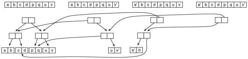
Figure 2: Sharing of subtrees in tree compression

When using a tree to store equal-length state vectors, compression is realized by the sharing of subtrees among entries. Fig. 2 illustrates this. Assuming that references have the same size as the slot values (say b bits), we can determine the compression rate in this example.

Storing one vector in a tree, requires storing information for the extra tree nodes, resulting in a total of $8b+(4-1)\times 2b=14b$ (not taking into account any implementation overhead from lookup structures). Each additional vector, however, can potentially share parts of the subtree with already-stored vectors. The second and third, in the example, only require a total of $6b$ each and the fourth only $2b$. The four vectors would occupy $4\times 8b=32b$ when stored in a normal hash table. This gives a compression ratio of $28b/32b=7/8$, likely to improve with each additional vector that is stored. Databases that store longer vectors also achieve higher compression rates as we will investigate later.

2.3 Why Parallelization is not Trivial

Adding generic compression techniques to the above algorithm can be done locally by adding a line compr := compress(succ) after l.9, and storing compr in DB. This calculation in compress only depends on succ and is therefore easy to parallelize. If, however, a form of informed compression is used, like Collapse or tree compression, the compressed value comes to depend on previously inserted state parts, and the compress function needs (multiple) accesses to the storage.

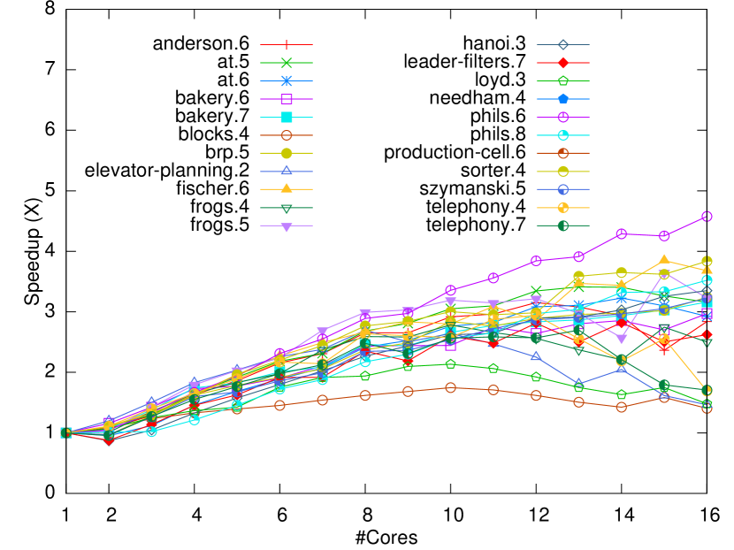
Figure 3: Speedup with Collapse.

Global locking or even locking at finer levels of granularity can be devastating for multi-core performance for single hash table lookups [14]. Informed compression algorithms, however, need multiple accesses and thus require careful attention when parallelized. Fig. 3 shows that Spin’s Collapse suffers from scalability problems (experimental settings can be found in Sec. 5).

3 Tree Database

Sec. 3.1 first describes the original tree compression algorithm from [1]. In Sec. 3.2, maximal sharing among tree nodes is introduced by merging the multiple hash tables of the tree into a single fixed-size table. By simplifying the data structure in this way, we aid scalability. Furthermore, we prove that it preserves consistency of the database’s content. However, as we also show, the new tree will “confuse” tree nodes and erroneously report some vectors as seen, while in fact they are new. This is corrected by tagging root tree nodes, completing the parallelization.

Sec. 3.3 shows how tree references can also be used to compact the size of the open set in Alg. 1. Now that the necessary space reductions are obtained, the current section is concluded with an algorithm that improves the performance of the tree database by using thread-local incremental information from the reachability search (Sec. 3.4).

3.1 Basic Tree Database

The tuples shown in Fig. 2 are stored in hash tables, creating a balanced binary tree of tables. Such a tree has $k-1$ tree nodes, each of which has a number of siblings of both the left and the right subtree that is equal or off by one. The tree_create function in Alg. 2 generates the Tree structure accordingly, with Nodes storing left and right subtrees, a Table table and the length of the (sub)tree $k$.

The tree_find_or_put function takes as arguments a Tree and a state vector $V$ (both of the same size $k>1$), and returns a tuple containing a reference to the inserted value and a boolean indicating whether the value was inserted before (seen, or else: new). The function is recursively called on half of the state vector (l.9-10) until the vector length is one. The recursion ends here and a single value of the vector is returned. At l.11, the returned values of the left and right subtree are stored as a tuple in the hash table using the table_find_and_put operation, which also returns a tuple containing a reference and a $seen/new$ boolean.

The function lhalf takes a vector $V$ as argument and returns the first half of the vector: $\mathsf{lhalf}(V)=[V_{0},\dots,V_{(\left\lceil{\frac{k}{2}}\right\rceil-1)}]$, and symmetrically $\mathsf{rhalf}(V)=[V_{\left\lceil{\frac{k}{2}}\right\rceil},\dots,V_{(k-1)}]$. So, $|\mathsf{lhalf}(V)|=\left\lceil{|V|/2}\right\rceil$, and $|\mathsf{rhalf}(V)|=\left\lfloor{|V|/2}\right\rfloor$.

⬇

1type Tree = Node(Tree left, Tree right, Table table, int k) | Leaf

2proc Tree tree_create(k)

3 if (k = 1)

4 return Leaf

5 return Node(tree_create($\left\lceil{\frac{k}{2}}\right\rceil$), tree_create($\left\lfloor{\frac{k}{2}}\right\rfloor$), Table(2), k)

6proc (int, bool) tree_find_or_put(Leaf, $V$)

7 return ($V[0]$, $\underline{\hskip 5.81247pt}$)

8proc (int, bool) tree_find_or_put(Node(left, right, table, k), $V$)

9 ($R_{\textrm{left}}$, $\underline{\hskip 5.81247pt}$) := tree_find_or_put(left, lhalf($V$))

10 ($R_{\textrm{right}}$, $\underline{\hskip 5.81247pt}$) := tree_find_or_put(right, rhalf($V$))

11 return table_find_or_put(table, $[R_{\textrm{left}},R_{\textrm{right}}]$)

Alg. 2: Tree data structure and algorithm for the tree_find_or_put function.

Implementation requirements.

A space-efficient implementation of the hash tables is crucial for good compression ratios. Furthermore, resizing hash tables are required, because the unpredictable and widely varying tree node sizes (tables may store a crossproduct of their children as shown in Sec. 4). However, resizing replaces entries, in other words, it breaks stable indexing, thus making direct references between tree nodes impossible. Therefore, in [1], stable indices were realized by maintaining a second table with references. Thus solving the problem, but increasing the number of cache misses and the storage costs per entry by 50%.

3.2 Concurrent Tree Database

Three conflicting requirements arise when attempting to parallelize Alg. 2: (1) resizing is needed because the load of individual tables is unknown in advance and varies highly, (2) stable indexing is needed, to allow for references to table entries, and (3) calculating a globally unique index concurrently is costly, while storing it requires extra memory as explained in the previous section.

An ideal solution would be to collapse all hash tables into a single non-resizable table. This would ensure stable indices without any overhead for administering them, while at the same time allowing the use of a scalable hash table design [14]. Moreover, it will enable maximal sharing of values between tree nodes, possibly further reducing memory requirements. But can all tree nodes safely be merged without corrupting the contents of the database?

To argue about consistency, we made a mathematical model of Alg. 2 with one merged hash table. The hash table uses stable indexing and is concurrent, hence each unique, inserted element will atomically yield one stable, unique index in the table. Therefore, we can describe table_find_or_put as a injective function: $H_{k}:\mathbb{N}^{k}\rightarrow\mathbb{N}$. The tree_find_or_put function can now be expressed as a recurrent relation ($T_{k}:\mathbb{N}^{k}\rightarrow\mathbb{N}$, for $k>1$ and $A\in\mathbb{N}^{k}$):
$T_{k}(A_{0},\dots,A_{(k-1)})=H_{2}(T_{\left\lceil{\frac{k}{2}}\right\rceil}(A_{0},\dots,A_{(\left\lceil{\frac{k}{2}}\right\rceil-1)}),T_{\left\lfloor{\frac{k}{2}}\right\rfloor}(A_{\left\lceil{\frac{k}{2}}\right\rceil},\dots,A_{(k-1)}))$
$T_{1}(A_{0})=A_{0}$.
We show that $T$ provides a similar injective function as $H$.

To prove (injection):

$C\equiv T_{k}(A)=T_{k}(B)\implies A=B$, with $A,B\in\mathbb{N}^{k}$.

Induction over $k$:

Base case: $T_{1}(x)=I(x)$, the identity function satisfies $C$ being injective. Assume $C$ holds $\forall i<k$ with $k>1$. We have to prove for all $A,B\in\mathbb{N}^{k}$, that:
$H_{2}(T_{\left\lceil{\frac{k}{2}}\right\rceil}(L(A)),T_{\left\lfloor{\frac{k}{2}}\right\rfloor}(R(A)))=H_{2}(T_{\left\lceil{\frac{k}{2}}\right\rceil}(L(B)),T_{\left\lfloor{\frac{k}{2}}\right\rfloor}(R(B)))\implies A=B$,
with $L(X)=X_{0},\dots,X_{(\left\lceil{\frac{k}{2}}\right\rceil-1)}$ and $R(X)=X_{\left\lceil{\frac{k}{2}}\right\rceil},\dots,X_{(k-1)}$. Note that:
$(*)\left\{\begin{array}[]{ll}L(A)=L(B)\land R(A)=R(B)\}$ if $A=B\\ L(A)\neq L(B)\lor R(A)\neq R(B)\}$ if $A\neq B$. Hence,$\\ \end{array}\right.$
$\left.\begin{array}[]{l}\left.\begin{array}[]{l}T_{k}(A)=T_{k}(B)\implies H_{2}(T_{\left\lceil{\frac{k}{2}}\right\rceil}(L(A)),T_{\left\lfloor{\frac{k}{2}}\right\rfloor}(R(A)))=H_{2}(T_{\left\lceil{\frac{k}{2}}\right\rceil}(L(B)),T_{\left\lfloor{\frac{k}{2}}\right\rfloor}(R(B)))\\ \stackrel{{\scriptstyle inj.H_{2}}}{{\implies}}T_{\left\lceil{\frac{k}{2}}\right\rceil}(L(A))=T_{\left\lceil{\frac{k}{2}}\right\rceil}(L(B))\land T_{\left\lfloor{\frac{k}{2}}\right\rfloor}(R(A))=T_{\left\lfloor{\frac{k}{2}}\right\rfloor}(R(B))\\ \stackrel{{\scriptstyle ind.hyp.}}{{\implies}}L(A)=L(B)\land R(A)=R(B)\stackrel{{\scriptstyle(*)}}{{\implies}}A=B\\ \end{array}\right.\\ \end{array}\right.$

Proving that $C$ holds for all $A$, $B$ and $k$. ∎

Now, it follows that an insert of a vector $A\in\mathbb{N}^{k}$ always yields a unique value for the root of the tree ($T_{k}$), thus demonstrating that the contents of the tree database are not corrupted by merging the hash tables of the tree nodes.

However, the above also shows that Alg. 2 will not always yield the right answer with merged hash tables. Consider: $T_{2}(A_{0},A_{1})=H_{2}(0,0)=T_{k}(A_{0},\dots,A_{(k-1)})$. In this case, when the root node $T_{k}$ is inserted into $H$, it will return a boolean indicating that the tuple $(0,0)$ was already seen, as it was inserted for $T_{2}$ earlier.

⬇

1type ConcurrentTree = CTree(Table table, int k)

2proc (int, bool) tree_find_or_put(tree, $V$)

3 $R$ := tree_rec(tree, $V$)

4 $B$ := if CAS($R$.tag, non_root, is_also_root) then new else seen

5 return ($R$, $B$)

6proc int tree_rec(CTree(table, k), $V$)

7 if (k = 1)

8 return $V[0]$

9 $R_{\textrm{left}}$ := tree_rec(CTree(table, $\left\lceil{\frac{k}{2}}\right\rceil$), lhalf($V$))

10 $R_{\textrm{right}}$ := tree_rec(CTree(table, $\left\lfloor{\frac{k}{2}}\right\rfloor$), rhalf($V$))

11 ($R$, $\underline{\hskip 5.81247pt}$) := table_find_or_put(table, $[R_{\textrm{left}},R_{\textrm{right}}]$)

12 return $R$

Alg. 3: Data structure and algorithm for parallel tree_find_or_put function.

Nonetheless, we can use the fact that $T_{k}$ is an injection to create a concurrent tree database by adding one bit (a tag) to the merged hash table. Alg. 3 defines a new ConcurrentTree structure, only containing the merge table and the length of the vectors $k$. It separates the recursion in the tree_rec function, which only returns a reference to the inserted node. The tree_find_or_put function now atomically flips the tag on the entry (the tuple) pointed to by $R$ in table from non_root to is_also_root, if it was not non_root before (see l.4). To this end, it employs the hardware primitive compare-and-swap (CAS), which takes three arguments: a memory location (in this case, $R.\mathit{tag}$), an old value and a designated value. CAS atomically compares the value val at the memory location with old, if equal, val is replaced by designated and true is returned, if not, false is returned.

Figure 4: Memory layout for CTree(Table, 4) with $\langle{a,b,c,d}\rangle$ inserted.

Implementation considerations.

Crucial for efficient concurrency is memory layout. While a bit array or sparse bit vector may be used to implement the tags (using $R$ as index), its parallelization is hardly efficient for high-throughput applications like reachability analysis. Each modified bit will cause an entire cache line (with typically thousands of other bits) to become dirty, causing other CPUs accessing the same memory region to be forced to update the line from main memory. The latter operation is multiple orders of magnitude more expensive than normal (cached) operations. Therefore, we merge the bit array/vector into the hash table table as shown in Fig 4, for this increases the spatial locality of node accesses with a factor proportional to the width of tree nodes. The small column on the left represents the bit array with black entries indicating is_also_root. The appropriate size of $b$ is discussed in Sec. 4.

Furthermore, we used the lockless hash table presented in [14], which normally uses memoized hashes in order to speed up probing over larger keys. Since the stored tree nodes are relatively small, we dropped the memoize hashes, demonstrating that this hash table design also functions well without additional memory overhead.

3.3 References in the Open Set

Now that tree compression reduces the space required for state storage, we observed that the open sets of the parallel reachability algorithm can become a memory bottleneck [15]. A solution is to store references to the root tree node in the open set as illustrated by Alg. 4, which is a modification of l.5-11 from Alg. 1.

⬇

1while (ref := $S_{id}.$get())

2 state := tree_get(DB, ref)

3 for (succ $\in$ next_state(state))

4 (newref, seen) := tree_find_or_put(DB, succ)

5 if ($\neg$seen)

6 $S_{id}$.put(newref)

Alg. 4: Reachability analysis algorithm with references in the open set.

The tree_get function is shown in Alg. 5. It reconstructs the vector from a reference. References are looked up in table using the table_get function, which returns the tuple stored in the table. The algorithm recursively calls itself until $k=1$, at this point ref_or_val is known to be a slot value and is returned as vector of size 1. Results then propagate back up the tree and are concatenated on l.7, until the full vector of length $k$ is restored at the root of the tree.

⬇

1proc int$[]$ tree_get(CTree(table, k), val_or_ref)

2 if (k = 1)

3 return $[$val_or_ref$]$

4 $[R_{\textrm{left}}$, $R_{\textrm{right}}]$ := table_get(table, val_or_ref)

5 $V_{\textrm{left}}$ := tree_get(CTree(table, $\left\lceil{\frac{k}{2}}\right\rceil$), $R_{\textrm{left}}$)

6 $V_{\textrm{right}}$ := tree_get(CTree(table, $\left\lfloor{\frac{k}{2}}\right\rfloor$), $R_{\textrm{right}}$)

7 return concat($V_{\textrm{left}}$, $V_{\textrm{right}}$)

Alg. 5: Algorithm for tree vector retrieval from a reference

3.4 Incremental Tree Database

The time complexity of the tree compression algorithm, measured in the number of hash table accesses, is linear in the number of state slots. However, because of today’s steep memory hierarchies these random memory accesses are expensive. Luckily, the same principle that tree compression exploits to deliver good state compression, can also be used to speedup the algorithm. The only entries that need to be inserted into the node table are the slots that actually changed with regard to the previous state and the tree paths that lead to these nodes. For a state vector of size $k$, the number of table accesses can be brought down to $\log_{2}(k)$ (the height of the tree) assuming only one slot changed. When $c$ slots change, the maximum number of accesses is $c\times\log_{2}(k)$, but likely fewer if the slots are close to each other in the tree (due to shared paths to the root).

Alg. 6 is the incremental variant of the tree_find_or_put function. The callee has to supply additional arguments: $P$ is the predecessor state of $V$ ($V\in\textsf{next\_state}(P)$ in Alg. 1) and RTree is a ReferenceTree containing the balanced binary tree of references created for $P$. RTree is also updated with the tree node references for $V$. tree_find_or_put needs to be adapted to pass the arguments accordingly.

⬇

1type ReferenceTree = RTree(ReferenceTree left, ReferenceTree right, int ref) | Leaf

2proc (int, bool) tree_rec(CTree(table, k), $V$, $P$, Leaf)

3 return ($V[0]$, $V[0]=P[0]$)

4proc (int, bool) tree_rec(CTree(table, k), $V$, $P$, inout RTree(left, right, ref))

5 ($R_{\textrm{left}}$, $B_{\textrm{left}}$) := tree_rec(CTree(table, $\left\lceil{\frac{k}{2}}\right\rceil$), lhalf($V$), lhalf($P$), left)

6 ($R_{\textrm{right}}$, $B_{\textrm{right}}$) := tree_rec(CTree(table, $\left\lfloor{\frac{k}{2}}\right\rfloor$), rhalf($V$), rhalf($P$), right)

7 if ($\neg B_{\textrm{left}}\lor\neg B_{\textrm{right}}$)

8 (ref, $\underline{\hskip 5.81247pt}$) := table_find_or_put$($table, $[R_{\textrm{left}},R_{\textrm{right}}]$)

9 return (ref, $B_{\textrm{left}}\land B_{\textrm{right}}$)

Alg. 6: ReferenceTree structure and incremental tree_rec function.

The boolean in the return tuple now indicates thread-local similarities between subvectors of $V$ and $P$ (see l.3). This boolean is used on l.7 as a condition for the hash table access; if the left or the right subvectors are not the same, then RTree is updated with a new reference that is looked up in table. For initial states, without predecessor states, the algorithm can be initialized with an imaginary predecessor state $P$ and tree RTree containing reserved values, thus forcing updates.

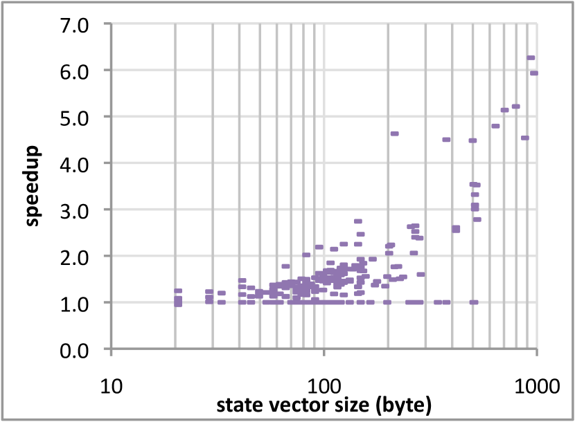
Figure 5: Speedup of Alg. 6 wrt. Alg. 3.

We measured the speedup of the incremental algorithm compared to the original (for the experimental setup see Sec. 5). Fig. 5 shows that the speedup is linearly dependent on $\log(k)$, as expected.

The incremental tree_find_or_put function changed its interface with respect to Alg. 3. Alg. 7 presents a new search algorithm (l.5-11 in Alg. 1) that also records the reference tree in the open set. RTree refs has become an input of the tree database, because it is also an output, it is copied to new_refs.

⬇

1while ((prev, refs) := $S_{id}.$get())

2 for (next $\in$ next_state(prev))

3 new_refs := copy(refs)

4 ($\underline{\hskip 5.81247pt}$, seen) := tree_find_or_put(DB, next, prev, new_refs)

5 if ($\neg$seen)

6 $S_{id}$.put((next, new_refs))

Alg. 7: Reachability analysis algorithm with incremental tree database.

Because the internal tree node references are stored, Alg.7 increases the size of the open set by a factor of almost two. To remedy this, either the tree_get function (Alg. 5) can be adapted to also return the reference trees, or the tree_get function can be integrated into the incremental algorithm (Alg. 6). (We do not present such an algorithm due to space limitations.) We measured little slowdown due to the extra calculations and memory references introduced by the tree_get algorithm (about 10% across a wide spectrum of input models).

4 Analysis of Compression Ratios

In the current section, we establish the minimum and maximum compression ratio for tree and Collapse compression. We count references and slots as stored in tuples at each tree node (a single such node entry thus has size 2). We fix both references and slots to an equal size.

Tree compression.

The worst case scenario occurs when storing a set of vectors $S$ with each $k$ identical slot values ($S=\{\langle{s,\dots,s}\rangle\mid s\in\{1,\dots,|S|\}\}$) [1]. In this case, $n=|S|$ and storing each vector $v\in S$ takes $2(k-1)$ ($k-1$ node entries). The compression is: $(2(k-1)n)/(nk)=2-2/k$. Occupying more tree entries is impossible, so always strictly less than twice the memory of the plain vectors is used.

Blom et al. [1] also give an example that results in good tree compression: the storage of the cross product of a set of vectors $S=P\times P$, where P consists of $m$ vectors of length $j=\frac{1}{2}k$. The cross product ensures maximum reuse of the left and the right subtree, and results in $n=|S|=|P|^{2}=m^{2}$ entries in only the root node. The left subtree stores $(j-1)|P|$ entries (taking naively the worst case), as does the right, resulting in a total of of $|S|+2(j-1)|P|$ tree node entries. The size of the tree database for S becomes $2n+2m(k-2)$. The compression ratio is $2/k+2/m-4/(mk)$ (divide by $nk$), which can be approximated by $2/k$ for sufficiently large n (and hence m). Most vectors can thus be compressed to a size approaching that of one node entry, which is logical since each new vector receives a unique root node entry (Sec. 3.2) and the other node entries are shared.

The optimal case occurs when all the individual tree nodes store cross products of their subtrees. This occurs when the value distribution is equal over all slots: $S=\{\langle{s_{0},\dots,s_{k-1}}\rangle\mid s_{i}\in\{1,\dots,\sqrt[k]{n}\}\}$ and that $k=2^{x}$. In this situation, the $\frac{k}{2}$ leaf nodes of the tree each receive $\sqrt[k/2]{n}$ entries: $\{\langle{s_{i},s_{i+1}}\rangle\mid i=2k\}$. The nodes directly above the leafs, receive each the cross product of that as entries, etc, until the root node which receives $n$ entries (see Fig. 6).

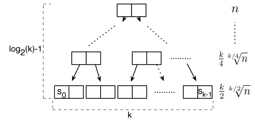
Figure 6: Optimal entries per tree node level.

With this insight, we could continue to calculate the total node entries for the optimal case and try to deduce a smaller lower bound, but we can already see that the difference between the optimal case and the previous case is negligible, since: $n+\sqrt{n}(k-2)-(n+2\sqrt{n}+4\sqrt[4]{n}+\ldots(\log_{2}(k)$ times$)\ldots+\frac{2}{k}\sqrt[2/k]{n})\ll n+\sqrt{n}(k-2)$, for any reasonably large n and k. From the comparison between the good and optimal case, we can conclude that only a cross product of entries in the root node is already near-optimal; the only way to get bad compression ratios may be when two related variables are located at different halves of the state vector.

Collapse compression.

Since the leafs of the process table are directly connected to the root, the compression ratios are easier to calculate. To yield optimal compression for the process table, a more restrictive scenario, than described for the tree above, needs to occur. We require $p$ symmetrical processes with each a local vector of $m$ slots ($k=p\times m$). Related slots may only lay within the bounds of these processes, take $S_{m}=\{\langle{s,\dots,s}\rangle\mid s\in\{1,\dots,|S_{m}|\}\}$. Each combination of different local vectors is inserted in the root table (also if $S_{m}=\{\langle{s,1,\dots,1}\rangle\mid s\in\{1,\dots,|S_{m}|\}\}$), yielding $n=|S_{m}|^{p}$ root table entries. The total size of the process table becomes $pn+m\sqrt[p]{n}$. The compression ratio is $(pn+m\sqrt[p]{n})/nk=\frac{p}{k}+m\frac{\sqrt[p]{n}}{nk}$. For large $n$ (hence $m$), the ratio approaches $\frac{p}{k}$.

Comparison.

Tab. 1 lists the achieved compression ratio for states, as stored in a normal hash table, a process table and a tree database under the different scenarios that were sketched before. It shows that the worst case of the process table is not as bad as the worst case achieved by the tree. On the other hand, the best case scenario is not as good as that from the tree, which compresses in this case to a fixed constant. We also saw that the tree can reach near-optimal cases easily, placing few constraints on related slots (on the same half). Therefore, we can expect the tree to outperform the compression of process table in more cases, because the latter requires more restrictive conditions. Namely, related slots can only be within the fixed bounds of the state vector (local to one process).

Table 1: Theoretical compression ratios of Collapse and tree compression.

Structure	Worst case	Best case
Hash table [14]	$1$	$1$
Process table	$1+\frac{p}{k}$	$\frac{p}{k}$
Tree database (Alg. 2, 3)	$2-\frac{2}{k}$	$\frac{2}{k}$

In practice.

With a few considerations, the analysis of this section can be applied to both the parallel and the sequential tree databases: (1) the parallel algorithm uses one extra tag bit per node entry, causing insignificant overhead, and (2) maximal sharing invalidates the worst-case analysis, but other sets of vectors can be thought up to still cause the same worst-case size. In practice, we can expect little gain from maximal sharing, since the likelihood of similar subvectors decreases rapidly the larger these vectors are, while we saw that the most node entries are likely near the top of the tree (representing larger subvectors). (3) The original sequential version uses an extra reference per node entry of overhead (50%!) to realize stable indexing (Sec. 3.1). Therefore, the proposed concurrent tree implementation even improves the compression ratio by a constant factor.

5 Experiments

We performed experiments on an AMD Opteron 8356 16-core ($4\times 4$ cores) server with 64 GB RAM, running a patched Linux 2.6.32 kernel. All tools were compiled using gcc 4.4.3 in 64-bit mode with high compiler optimizations (-O3).

We measured compression ratios and performance characteristics for the models of the Beem database [18] with three tools: DiVinE 2.2, Spin 5.2.5 and our own model checker LTSmin [3, 15]. LTSmin implements Alg. 3 using a specialized version of the hash table [14] which inlines the $tags$ as discussed at the end of Sec. 3.2. Special care was taken to keep all parameters across the different model checkers the same. The size of the hash/node tables was fixed at $2^{28}$ elements to prevent resizing and model compilation options were optimized on a per tool basis as described in earlier work [3]. We verified state and transition counts with the Beem database and DiVinE 2.2. The complete results with over 1500 benchmarks are available online[13].

5.1 Compression Ratios

For a fair comparison of compression ratios between Spin and LTSmin, we must take into account the differences between the tools. The Beem models have been written in DVE format (DiVinE) and translated to Promela. The translated Beem models that Spin uses may have a different state vector length. LTSmin reads DVE inputs directly, but uses a standardized internal state representation with one 32-bit integer per state slot (state variable) even if a state variable could be represented by a single byte. Such an approach was chosen in order to reuse the model checking algorithms for other model inputs (like mCRL, mCRL2 and DiVinE [2]). Thus, LTSmin can load Beem models directly, but blows up the state vector by an average factor of three. Therefore, we compare the average compressed state vector size instead of compression ratios.

Table 2: Original and compressed state sizes and memory usage for LTSmin with hash table (Table), Collapse (Spin) and our tree compression (Tree) for a representative selection of all benchmarks.

Model	Orig. State [Byte]		Compr. State [Byte]		Memory [MB]
	Spin	Tree	Spin	Tree	Table	Spin	Tree
at.6	68	56	36.9	8.0	8,576	4,756	1,227
iprotocol.6	164	148	39.8	8.1	5,842	2,511	322
at.5	68	56	37.1	8.0	1,709	1,136	245
bakery.7	48	80	27.4	8.8	2,216	721	245
hanoi.3	116	228	112.1	13.8	3,120	1,533	188
telephony.7	64	96	31.1	8.1	2,011	652	170
anderson.6	68	76	31.7	8.1	1,329	552	140
frogs.4	68	120	73.2	8.2	1,996	1,219	136
phils.6	140	120	58.5	9.3	1,642	780	127
sorter.4	88	104	39.7	8.3	1,308	501	105
elev_plan.2	52	140	67.1	9.2	1,526	732	100
telephony.4	54	80	28.7	8.1	938	350	95
fischer.6	92	72	43.7	8.4	571	348	66

Table 2 shows the uncompressed and compressed vector sizes for Collapse and tree compression. Tree compression achieves better and almost constant state compression than Collapse for these selected models, even though original state vectors are larger in most cases. This confirms the results of our analysis.

We also measured peak memory usage for full state space exploration. The benefits with respect to hash tables can be staggering for both Collapse and tree compression: while the hash table column is in the order of gigabytes, the compressed sizes are in the order of hundreds of megabytes. An extreme case is hanoi.3, where tree compression, although not optimal, is still an order of magnitude better than Collapse using only 188 MB compared to 1.5 GB with Collapse and 3 GB with the hash table.

To analyze the influence of the model on the compression ratio, we plotted the inverse of the compression ratio against the state length in Fig. 7. The line representing optimal compression is derived from the analysis in Sec. 4 and is linearly dependent on the state size (the average compressed state size is close to 8 bytes: two 32-bit integers for the dominating root node entries in the tree).

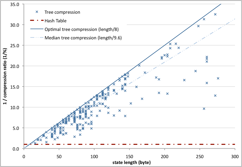
Figure 7: Compression ratios for 279 models of the Beem database are close to optimal for tree compression.

With tree compression, a total of 279 Beem models could each be fully explored using a tree database of pre-configured size, never occupying more than 4 GB memory. Most models exhibit compression ratios close to optimal; the line representing the median compression ratio is merely 17% below the optimal line. The worst cases, with a ratio of three times the optimal, are likely the result of combinatorial growth concentrated around the center of the tree, resulting in equally sized root, left and right sibling tree nodes. Nevertheless, most sub-optimal cases lie close too half of the optimal, suggesting only one “full” sibling of the root node. (We verified this to be true for several models.)

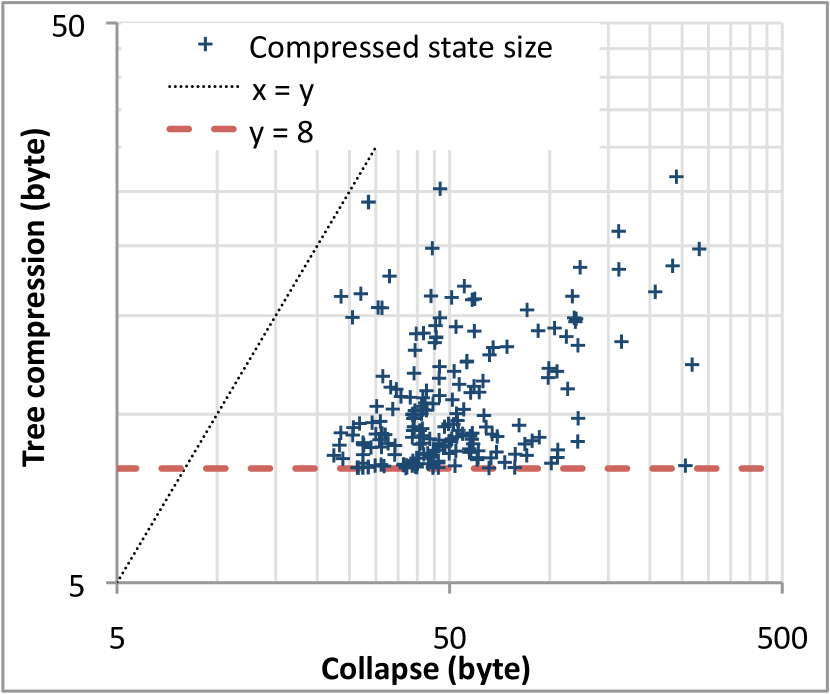
Figure 8: Log-log scatter plot of Collapse and tree-compressed state sizes (smaller is better): for all tested models, tree compression uses less memory.

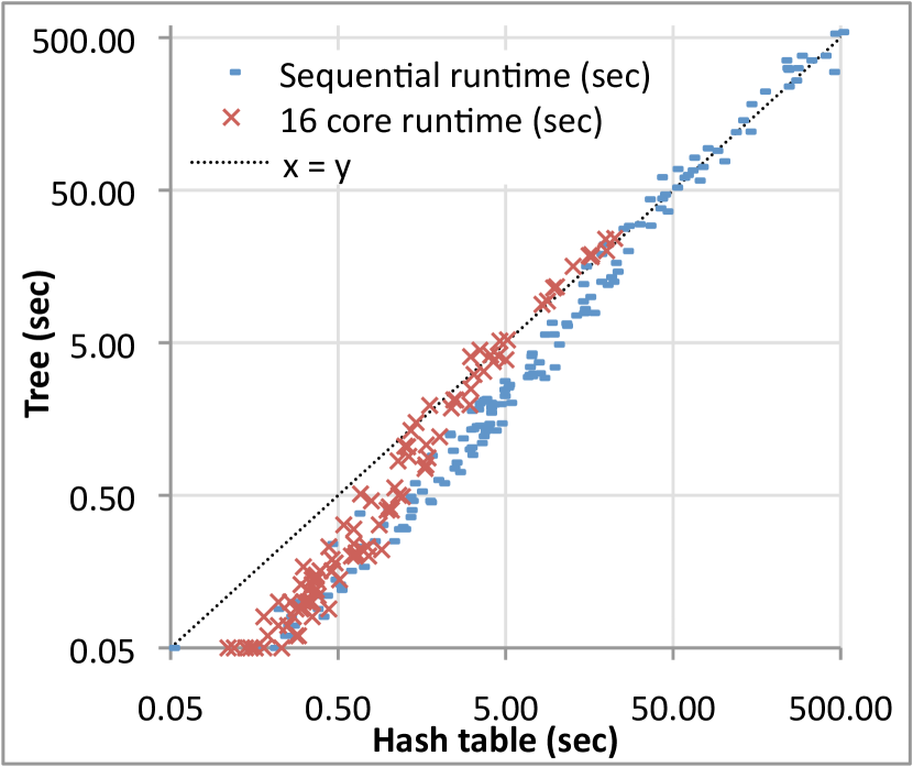
Figure 9: Log-log scatter plot of LTSmin run-times for state space exploration with either a hash table or tree compression.

Fig. 9 compares compressed state size of Collapse and tree compression. (We could not easily compare compressed state space sizes due to differing number of states for some models). Tree compression performs better for all models in our data set. In many cases, the difference is an order of magnitude. While tree compression has an optimal compression ratio that is four times better than Collapse’s (empirically established), the median is even five times better for the models of the Beem database. Finally, as expected (see Sec. 4), we measured insignificant gains from the introduced maximal sharing.

5.2 Performance & Scalability

We compared the performance of the tree database with a hash table in DiVinE and LTSmin. A comparison with Spin was already provided in earlier work [14]. For a fair comparison, we modified a version of LTSmin to use the (three times) shorter state vectors (char vectors) of DiVinE directly. Fig. 10 shows the total runtime of 158 Beem models, which fitted in machine memory using both DiVinE and LTSmin. On average the run-time performance of tree compression is close to a hash table-based search (see Fig. 10(a)). However, the absolute speedup in Fig. 10(b) shows that scalability is better with tree compression, due to a lower memory footprint.

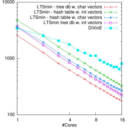
(a) Total runtime

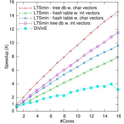
(b) Average (absolute) speedup

Figure 10: Performance benchmarks for 158 models with DiVinE (hash table) and with LTSmin using tree compression and hash table.

Fig. 9 compares the sequential and multi-core performance of the fastest hash table implementation (LTSmin lockless hash table with char vectors) with the tree database (also with char vectors). The tree matches the performance of the hash table closely.

For both, sequential and multi-core, the performance of the tree database is nearly the same as the fastest hash table implementation, however, with significantly lower memory utilization. For models with fewer states, tree database performance is better than a hash table, undoubtedly due to better cache utilization and lower memory bandwidth.

6 Conclusions

First, this paper presented an analysis and experimental evaluation of the compression ratios of tree compression and Collapse compression, both informed compression techniques that are applicable in on-the-fly model checking. Both analysis and experiments can be considered an implementation-independent comparison of the two techniques. Collapse compression was considered the state-of-the-art compression technique for enumerative model checking. Tree compression was not evaluated as such before. The latter is shown here to perform better than the former, both analytically and in practice. In particular, the median compression ratio of tree compression is five times better than that of Collapse on the Beem benchmark set. We consider this result representative to real-world usage, due to the varied nature of the Beem models: the set includes models drawn from extensive case studies on protocols and control systems, and, implementations of planning, scheduling and mutual exclusion algorithms [17].

Furthermore, we presented a solution for parallel tree compression by merging all tree-node tables into a single large table, thereby realizing maximal sharing between entries in these tables. This single hash table design even saves 50% in memory because it exhibits the required stable indexing without any bookkeeping. We proved that the consistency is maintained and use only one bit per entry to parallelize tree insertions. Lastly, we presented an incremental tree compression algorithm that requires a fraction of the table accesses (typically $\mathcal{O}(\log_{2}(k))$, i.e., logarithmic in the length of a state vector), compared to the original algorithm.

Our experiments show that the incremental and parallel tree database has the same performance as the hash table solutions in both LTSmin and DiVinE (and by implication Spin [14]). Scalability is also better. All in all, the tree database provides a win-win situation for parallel reachability problems.

Discussion.

The absence of resizing could be considered a limitation in certain applications of the tree database. In model checking, however, we may safely dedicate the vast majority of available memory of a system to the state storage.

The current implementation of LTSmin [20] supports a maximum of $2^{32}$ tree nodes, yielding about $4\times 10^{9}$ states with optimal compression. In the future, we aim to create a more flexible solution that can store more states and automatically scales the number of bits needed per entry, depending on the state vector size. What has hold us back thus far from implementing this are low-level issues, i.e., the ordering of multiple atomic memory accesses across cache line boundaries behave erratically on certain processors.

While this paper discusses tree compression mainly in the context of reachability, it is not limited to this context. For example, on-the-fly algorithms for the verification of liveness properties can also benefit from a space-efficient storage of states as demonstrated by Spin with its Collapse compression.

Future Work.

A few options are still open to improve tree compression. The small tree node entries cover a limited universe of values: $1+2\times\log_{2}(n)$. This is an ideal case to employ key quotienting using Cleary [6] or Very Tight Hashtables [10]. Neither of the two techniques has been parallelized as far as we can tell.

Static analysis of the dependencies between transitions and state slots could be used to reorder state slots and obtain a better balanced tree, and hence better compression (see Sec. 4). Much like the variable ordering problem of BDDs [5], finding the optimal reordering is an exponential problem (a search through all permutations). While, we are able to improve most of the worse cases by automatic variable reordering, we did not yet find a good heuristic for at least all Beem models.

Finally, it would be interesting to generalize the tree database by accommodating for the storage of vectors of different sizes.

Acknowledgements

We thank Elwin Pater for taking the time to proofread this work and provide feedback. We thank Stefan Blom for the many useful ideas that he provided.

References

- [1] S.C.C. Blom, B. Lisser, J.C. van de Pol, and M. Weber. A database approach to distributed state space generation. In Sixth International Workshop on Parallel and Distributed Methods in verifiCation, PDMC, pages 17–32, Enschede, July 2007. CTIT.
- [2] S.C.C. Blom, J.C. van de Pol, and M. Weber. Bridging the gap between enumerative and symbolic model checkers. Technical Report TR-CTIT-09-30, University of Twente, Enschede, June 2009.
- [3] S.C.C. Blom, J.C. van de Pol, and M. Weber. LTSmin: Distributed and symbolic reachability. In T. Touili, B. Cook, and P. Jackson, editors, Computer Aided Verification, Edinburgh, volume 6174 of Lecture Notes in Computer Science, pages 354–359, Berlin, July 2010. Springer Verlag.
- [4] S.C.C. Blom, I. van Langevelde, and B. Lisser. Compressed and distributed file formats for labeled transition systems. Electronic Notes in Theoretical Computer Science, 89(1):68 – 83, 2003. PDMC 2003, Parallel and Distributed Model Checking (Satellite Workshop of CAV ’03).
- [5] R.E. Bryant. Symbolic boolean manipulation with ordered binary-decision diagrams. ACM Comput. Surv., 24(3):293–318, 1992.
- [6] J.G. Cleary. Compact hash tables using bidirectional linear probing. IEEE Transactions on Computers, 33:828–834, 1984.
- [7] T.M. Cover and J.A. Thomas. Elements of Information Theory. Wiley-Interscience, 99th edition, August 1991.
- [8] S. Evangelista and J.F. Pradat-Peyre. Memory efficient state space storage in explicit software model checking. In Patrice Godefroid, editor, Model Checking Software, volume 3639 of Lecture Notes in Computer Science, pages 43–57. Springer Berlin / Heidelberg, 2005.
- [9] J. Geldenhuys, P. de Villiers, and J. Rushby. Runtime efficient state compaction in SPIN. In Dennis Dams, Rob Gerth, Stefan Leue, and Mieke Massink, editors, Theoretical and Practical Aspects of SPIN Model Checking, volume 1680 of Lecture Notes in Computer Science, pages 12–21. Springer Berlin / Heidelberg, 1999.
- [10] J. Geldenhuys and A. Valmari. A nearly memory-optimal data structure for sets and mappings. In SPIN’03: Proceedings of the 10th international conference on Model checking software, pages 136–150, Berlin, Heidelberg, 2003. Springer-Verlag.
- [11] G.J. Holzmann. State compression in SPIN: Recursive indexing and compression training runs. In proc. of the third international SPIN workshop, 1997.
- [12] G.J. Holzmann, P. Godefroid, and D. Pirottin. Coverage preserving reduction strategies for reachability analysis. In Proceedings of the IFIP TC6/WG6.1 Twelth International Symposium on Protocol Specification, Testing and Verification XII, pages 349–363, Amsterdam, The Netherlands, 1992. North-Holland Publishing.
- [13] A.W. Laarman. LTSmin benchmark results. http://fmt.cs.utwente.nl/tools/ltsmin/spin-2011/, 2011. Last accessed: 24 Jan 2011.
- [14] A.W. Laarman, J.C. van de Pol, and M. Weber. Boosting multi-core reachability performance with shared hash tables. In N. Sharygina and R. Bloem, editors, Proceedings of the 10th International Conference on Formal Methods in Computer-Aided Design, Lugano, Switzerland, USA, October 2010. IEEE Computer Society.
- [15] A.W. Laarman, J.C. van de Pol, and M. Weber. Multi-core ltsmin: Marrying modularity and scalability. In M. Bobaru, K. Havelund, G. Holzmann, and R. Joshi, editors, Proceedings of the Third International Symposium on NASA Formal Methods, NFM 2011, Pasadena, CA, USA, volume 6617 of LNCS, pages 506–511, Berlin, July 2011. Springer Verlag.
- [16] K. Larsen, F. Larsson, P. Pettersson, and W. Yi. Efficient verification of real-time systems: Compact data structure and state–space reduction. In Proc. of the 18th IEEE Real-Time Systems Symposium, pages 14–24. IEEE Computer Society Press, 1997.
- [17] R. Palének. The BEEM website. http://anna.fi.muni.cz/models/cgi/models.cgi, 2011. Last accessed: 24 Jan 2011.
- [18] R. Pelánek. BEEM: Benchmarks for explicit model checkers. In Proc. of SPIN Workshop, volume 4595 of LNCS, pages 263–267. Springer, 2007.
- [19] P. Sanders. Lastverteilungsalgorithmen fur parallele tiefensuche. number 463. In Fortschrittsberichte, Reihe 10. VDI. Verlag, 1997.
- [20] M. Weber. The LTSmin website. http://fmt.cs.utwente.nl/tools/ltsmin/, 2011. Last accessed: 24 Jan 2011.