Weak ferromagnetism of antiferromagnetic domains in graphene with defects

Abstract

Magnetic properties of graphene with randomly distributed magnetic defects/vacancies are studied in terms of the Kondo Hamiltonian in the mean field approximation. It has been shown that graphene with defects undergoes a magnetic phase transition from a paramagnetic to a antiferromagnetic (AFM) phase once the temperature reaches the critical point $T_{N}$. The defect straggling is taken into account as an assignable cause of multiple nucleation into AFM domains. Since each domain is characterized by partial compensating magnetization of the defects associated with different sublattices, together they reveal a super-paramagnetic behavior in a magnetic field. Theory qualitatively describe the experimental data provided the temperature dependence of the AFM domain structure.

Along with unique transport characteristics the magnetic behavior of the graphene-based materials attracts much attention in recent studies due to the significant interest in fundamental physics and prospective spintronic applications. Particularly, the possibility of the band gap manipulating in antiferromagnetic ordered defective graphene (i.e. graphene with adatoms or vacancies)Daghofer10 ; Rappoport10 ; Balog10 offers an additional control for nonlinear functionality while an efficient spin injection capability into grapheneKawakami10 with long spin coherence time/length even at room temperature Tombros07 puts the graphene in the forefront of the materials for emerging spin-based information processing. Furthermore, the room temperature weak ferromagnetism (FM) has been reported in highly oriented pyrolitic graphite irradiated by proton beamsEsquinazi03 and in defective graphene prepared from soluble functionalized graphene sheets.Wang09 Moreover, it was experimentally discovered the coexist of ferromagnetic correlations along with antiferromagnetic (AFM) interactions in all series of the multilayer defective graphene samples in Ref. Matte09, . On the other hand, no ferromagnetism has been detected in pure graphene nanocrystals in wide range of temperatures Sepioni10 revealing ambiguity about the graphene edge contribution to magnetization data (compare Refs. Yazyev08, ; Cervenka09, ; Lin09, ).

It was recently theoretically and experimentally realized that the vacancies or hydrogen addatoms associated with carbon atoms mediate the local magnetic moments in the graphene.Yazyev07 ; Kumazaki07 ; Pisani08 ; Palacios08 ; Yazyev10 Moreover, the local spin moments of the defects reveal strong exchange interaction with delocalized electrons that is the main source to trigger low temperature anomaly in conductivity and Kondo effect.Hentschel07 ; Zhu10 ; Fuhrer10 ; Uchoa10 Theoretical analysis of indirect interaction through the graphene carriers in terms of Kondo Hamiltonian unambiguously indicates the ferromagnetic (antiferromagnetic) exchange coupling between localized spins associated with the same (different) sublattices of the crystalline graphene.Brey07 ; Cheianov07 ; Rappoport09 ; Venezuela09 ; Schaffer10 This fact as well as Lieb’s theoremLeib are usually adduced to back up the arguments that a weak ferromagnetism is a result of imbalance $\Delta N_{d}$ in the number of vacancies/impurities of the A or B sublattices (i.e. not precise compensation of sublattices magnetizations with opposite directions).Easquinazi10 ; Lopez10 At the same time the actual imbalance of randomly distributed spin moments fails even a weak ferromagnetism because $\left|\Delta N_{d}\right|/N_{d}\rightarrow 0$ in large graphene crystal with the total number $N_{d}$ of the defects.

In present study we propose a different approach to the problem of coexistence of FM and AFM phase in a single graphene layer. It takes into account a multiple nucleation of antiferromagnetic domain germs in the mass of randomly distributed spins in monolayer graphene. At the same time, the domains each reveal a small random imbalance $\Delta n_{d}$ and magnetism so that together they additively contribute to the net magnetic moment culminating the saturated magnetization in a magnetic field. In such a way the finiteness of the magnetic correlations should be taken into account. The strong short-range correlation within each domain is responsible for its antiferromagnetic ordering. Such AFM correlations are weakened or broken at the domain boundaries, which can be associated with the impurity rarefactions or lattice imperfects. Thus the behavior of the magnetic domains in a magnetic field is almost mutually independent that constitutes some finite magnetization in the limit $N_{d}\rightarrow\infty$. It is important to note that magnetism in graphene does not come into conflict with Mermin-Wagner theorem Mermin66 because of finite magnetic anisotropy Brataas06 ; Yazyev08 and restricted sizes of AFM domains.

The microscopic approach is based on the Kondo Hamiltonian of carrier-localized spin exchange interaction that has been extensively used in the analysis of magnetic properties of graphene in Refs. Hentschel07, ; Uchoa10, ; Rappoport10, and Schaffer10, . The spectrum of bulk graphene is treated in tight binding approximation. In mean field approximation, this approach leads to set of two equations for the sublattice magnetizations that define a critical temperature of the antiferromagnetic ordering without any limitations on the number of carbon atoms involving to computation in more sophisticated models (Refs. Daghofer10, and Rappoport10, ). As a result, we find a simple analytical expression for Néel temperature that may serve as a guide for analysis of the numerous experimental data on graphene magnetism and estimate the mean size of the magnetic domains in graphene.

Let us consider a graphene fragment possessed large enough a flat area $A_{f}$ to neglect the edge effects. The Hamiltonian in momentum representation takes the form Neto09

$$H_{\mathbf{k}}=\gamma_{cc}[\widehat{\sigma}_{1}f_{1}(\mathbf{k})+\widehat{\sigma}_{2}f_{2}(\mathbf{k})],$$ (1)

where $\gamma_{cc}=2.7$ eV is the matrix element of electron hopping between nearest neighbor atoms connected with the vectors $\mathbf{e}_{m}$ ($m$=1,2,3), the Pauli matrixes $\widehat{\sigma}_{i}$ are defined over the sublattices $A$ and $B$ basic functions and $\mathbf{k=}(k_{x},k_{y})$ is the electron momentum; $f_{1}(\mathbf{k})=\sum_{m}\cos(\mathbf{k\mathbf{e}}_{m})$, $f_{2}(\mathbf{k})=\sum_{m}\sin(\mathbf{k\mathbf{e}}_{m})$. We assign $\mathbf{e}_{m}=a_{cc}(\cos m\omega,\sin m\omega)$, where $a_{cc}=0.142$ nm and $\omega=2\pi/3$. In diagonal form, Hamiltonian (1) describes the graphene dispersion law

$$\epsilon_{b,\mathbf{k}}=\gamma_{cc}b\varepsilon(a_{0}\mathbf{k})$$ (2)

for conduction ($b=1$) and valence ($b=-1$) bands with $\varepsilon(a_{0}\mathbf{k})=\sqrt{f_{1}^{2}(\mathbf{k})+f_{2}^{2}(\mathbf{k})}$. A straightforward algebra shows that $\varepsilon(\mathbf{q})=\left(3+4\cos\frac{\sqrt{3}q_{x}}{2}\cos\frac{q_{y}}{2}+2\cos q_{y}\right)^{1/2}$, i.e. there are two non-equivalent contact points at the corners of first Brillouin zone (BZ) $\mathbf{K,K}^{\prime}=\frac{\omega}{a_{0}}(\sqrt{3},\pm 1,)$ where conduction and valence bands are degenerated at $\epsilon_{b,\mathbf{K}}=\epsilon_{b,\mathbf{K}^{\prime}}=0$; $a_{0}=\sqrt{3}a_{cc}$ is a length of lattice vectors. In the vicinity of these points the energy dispersions are the Dirac cones, $\epsilon_{b,\mathbf{K}^{(\prime)}+\mathbf{\varkappa}}=b\hbar v_{F}\left|\mathbf{\varkappa}\right|$, with Fermi velocity $v_{F}=\frac{\sqrt{3}}{2}\gamma_{cc}a_{0}/\hbar$.

The Kondo Hamiltonian of the exchange interaction between a band electron (with position $\mathbf{r}$ and spin $\mathbf{S}$) and the $n_{d}$ localized spin moments $\mathbf{I}_{j}$ pinned to the sites $\mathbf{R}_{j}$ of the graphene lattice reads

$$H_{K}=-\sum_{j=1}^{n_{d}}J(\mathbf{r},\mathbf{R}_{j})\mathbf{I}_{j}\mathbf{S,}$$ (3)

where $J(\mathbf{r},\mathbf{R}_{j})\approx J\varpi_{0}\delta(\mathbf{r}-\mathbf{R}_{j})$, $J$ is the exchange constant, $n_{d}=n_{A}+n_{B}$ the total number of the defects located at $A$ and $B$ sublattices, $\varpi_{0}=\sqrt{3}a_{0}^{2}/2$. In the bipartite graphene lattice, it is convenient to double group the Hamiltonian of Eq. (3) on sublattice defects $j_{A(B)}=1,...,$ $n_{A(B)}$: $H_{K}=H_{K}^{(A)}+H_{K}^{(B)}$. In the representation of eigenfunctions of Eq. (1), each part of $H_{K}$ manifests itself through the projection operators $P_{A(B)}=(1\pm\widehat{\sigma}_{3})/2$. Then the summing up over the random scattered impurities and thermal averaging of their spin states reduce Eq. (3) to

$$H_{ex}=\alpha\mathbf{(m\mathbf{S+w}C),}$$ (4)

where the total magnetic moment of the defects $\mathbf{m}=\mathbf{m}_{A}+\mathbf{m}_{B}$ and their antiferromagnetic vector $\mathbf{w}=\mathbf{m}_{A}-\mathbf{m}_{B}$ are expressed via sublattice magnetic moments $\mathbf{m}_{A(B)}=-n_{A}g\mu_{B}\left\langle\mathbf{I}_{j_{A(B)}}\right\rangle$; $\alpha=\frac{1}{n_{f}}\frac{J}{g\mu_{B}}$, $n_{f}=A_{f}/\varpi_{0}$ the total number of primitive sells, $\varpi_{0}$ is their area, $g\cong 2$ and $\mu_{B}$ are the $g$-factor and Bohr magneton. The distinguishing property of Eq. (4) is that AFM vector exerts the composite spin $\mathbf{C}=\widehat{\sigma}_{3}\otimes\mathbf{S}$ that can be a finite magnitude even under $\left\langle\mathbf{S}\right\rangle=0$.

Let us introduce the effective magnetic fields $\mathbf{B}_{A}$ and $\mathbf{B}_{B}$ that cause the spin polarizations in each sublattice $\left\langle\mathbf{I}_{j_{A(B)}}\right\rangle=-\mathbf{n}_{A(B)}\frac{\mathbf{1}}{2}\tanh\frac{g\mu_{B}B_{A(B)}}{2T}$, $\mathbf{n}_{A(B)}=\mathbf{B}_{A(B)}/B_{A(B)}$, $k_{B}=1$. On the other hand they can be represented as LP9

$$\mathbf{B}_{A(B)}\mathbf{=}\mathbf{-}\frac{\partial\Phi}{\partial\mathbf{m}_{A(B)}}$$ (5)

in terms of of thermodynamic potential

$$\Phi=-T\sum_{b,s,\mathbf{k}}\ln\left(1+e^{(\mu-E_{b,s,k})/T}\right),$$ (6)

and chemical potential $\mu$. The energy bands of the defective graphene with Hamiltonian $H_{\mathbf{k}}+H_{ex}$ are described by

$$E_{b,s,\mathbf{k}}=\frac{s}{2}\alpha m+b\sqrt{\epsilon_{b,\mathbf{k}}^{2}+\left(\frac{\alpha w}{2}\right)^{2}},$$ (7)

where $s=\pm 1$ is a spin number. A distinctive feature of the dispersion law (7) consists in opening bandgap $E_{g}=\alpha(w-m)$ provided that $w>m$. Such splitting of the energy bands lowers the total electronic energy of the valence band that cannot be compensated by raising electron energy in the conduction band resembling the cooperative Jahn-Teller effect.Englman72 Equation (5) constitutes the closed set of the equations for both $\mathbf{B}_{A}=\widehat{\mathbf{z}}B_{A}$ and $\mathbf{B}_{B}=\widehat{\mathbf{z}}B_{B}$, the unit vector $\widehat{\mathbf{z}}$ is directed along quantization axis. Explicitly they take the form of integral over the first BZ,

$$B_{A,B} \mathbf{=} \mathbf{-}\frac{\varpi_{0}}{g\mu_{B}(2\pi)^{2}}\int\int_{BZ}dq_{x}dq_{y}F(\mathbf{k});$$ (8)

$$F(\mathbf{k}) = J\sum_{b,s}\left(\frac{s}{2}\pm\frac{b\alpha w}{4\sqrt{\epsilon_{b,\mathbf{k}}^{2}+\left(\frac{\alpha w}{2}\right)^{2}}}\right)f(E_{b,s,\mathbf{k}}-\mu),$$ (9)

where $f(E_{b,s,\mathbf{k}}-\mu)$ is the Fermi-Dirac function and $\pm$ discriminates the different sublattices.

In the first stage we focus on the stronger effect of AFM ordering within a single domain that eventually establishes weak FM. Ignoring small imbalance $\Delta n_{d}\ll n_{d}$, Eqs. (8) and (9) decompose on independent equations for $B_{A}$ and $B_{B}=-B_{A}$ so that each $B_{A}$ and $B_{B}$ satisfy to the self-consistent equation

$$y=\frac{J^{2}x}{T\gamma_{cc}}I(y,\mu,T)\tanh\left(\frac{y}{2}\right),$$ (10)

in terms of variable $y=g\mu_{B}B_{A(B)}/T$. A complex integral function $I(y,\mu,T)$ can be reduced with high accuracy to the constant $I_{0}\simeq 0.448$ provided that $\gamma_{cc}\gg Jx,\mu,T$. Therewith in the limit $y\rightarrow 0$ Eq. (10) gives rise the expression for Néel temperature

$$T_{N}=\frac{J^{2}x}{2\gamma_{cc}}I_{0},$$ (11)

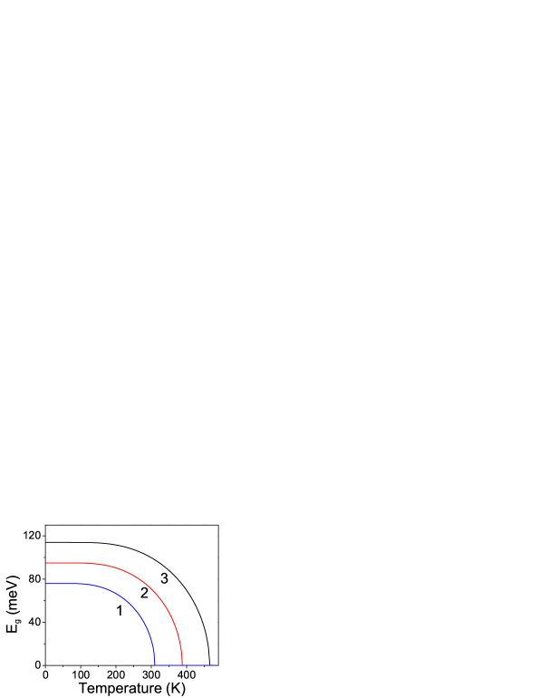
Figure 1: Band gap of the defective graphene vs temperature at $J=1.9$ eV and defect molar fractions 4%, 5% and 6% (curves 1, 2 and 3 respectively).

which depends merely on the exchange constant and defect fraction $x=n_{d}/2n_{f}$. The squared dependence of $T_{N}$ on $J$ as well as the quantitative evaluation $T_{N}=0.0112\gamma_{cc}$ at $x=0.2$ and $J=0.5\gamma_{cc}$ are in a good agreement with Monte-Carlo simulations carried out in Ref. Rappoport10, . Particulary, the Eq.(11) shows that exchange constant $\left|J\right|=1.9$ eV guarantees a room temperature AFM ordering at reasonable low $x=0.04$. Solutions $y=y(x,T)$ of Eq. (10) define also the energy gap $E_{g}=Jx\tanh\frac{y(x,T)}{2}$ and magnetization $m_{A}=\frac{1}{2}n_{A}g\mu_{B}\tanh\frac{y(x,T)}{2}$. Fig. 1 illustrate the temperature dependence of $E_{g}$ calculated with Eq. (10).

Nucleation of $N_{D}$ AFM domains each in possess of a random imbalance $n_{A}-n_{B}$ lays the groundwork for weak ferromagnetism in graphene. Applying the statistical approach, let us attribute $x$ to the equal probability for each site $A$ or $B$ to be defected for all $N_{D}$ domains so that mean number of deviation is $\overline{(n_{A}-n_{B})}=0$ because $\overline{n_{A}}=\overline{n_{B}}=xn_{f}$. The mean-square estimate is $\overline{(n_{A}-n_{B})^{2}}=2n_{f}x(1-x)=n_{d}(1-x)$, thus the mean number of non-compensated spins is$\overline{\text{ }\Delta n_{d}}=\sqrt{2n_{f}x(1-x)}=\sqrt{n_{d}(1-x)}$. The respective magnetic moment

$$m(n_{f},x,T)\simeq\mu_{B}\sqrt{2n_{f}x(1-x)}\tanh\frac{y(x,T)}{2}$$ (12)

can be interpreted as a weak ferromagnetism attributed to a single domain.

Above we considered the formation of the magnetic moments $m(n_{f},x,T)\leq$ $\mu_{B}\sqrt{n_{d}}$ ($n_{d}\gg\sqrt{n_{d}}\gg 1$) in individual AFM domains. To consider the behavior of multi-domain graphene in a magnetic field $\mathbf{B}_{0}$ further conjectures must be done. It is convenient to split the ensemble of domains on subsets, each determined by certain space $A_{f}$ and number $n_{d}$ of the defects. In a magnetic field $\mathbf{B}_{0}$ the $A_{f}$ -domain with $n_{d}$ defects contributes to the net magnetization as $m(n_{f},x,T)L[B_{0}m(n_{f},x,T)/T_{eff}]$, where $L(x)$ is a Langevin function and $T_{eff}=T+T_{AF}$ is an effective temperature. Parameter $T_{AF}$ takes into account the tendency to merge several small domains into one large AFM one that reveals a close analogy of this parameter with the temperature shift $T_{0}$ in diluted magnetic semiconductors with AFM interaction between localized spin moments.Bednarski00 Such interdomain interaction constitutes proportionality of $T_{AF}$ to the length of domain boundary network or inverse proportionality to domain mean size $L$. The final magnetization output $M$ can be expressed in terms of distribution function $f(A_{f},x)$ so that

$$M=\int\int m(n_{f},x,T)L\left(\frac{B_{0}m(n_{f},x,T)}{T_{eff}}\right)f(A_{f},x)dA_{f}dx.$$ (13)

Apparently the dispersion in the domain shapes and spaces and in the defect densities is very specific for particular sample preparation, chemical and thermal treatment; therefore the $f(A_{f},x)$ cannot be specified a priori. So in the rest part of the paper we focus on the analysis of particular experimental data on graphene magnetization reported in Ref. Wang09, . There was found that at room temperature, a magnetic field $B_{0}\approx 3$ kOe saturates magnetization at small amounts $M_{s}=0.02$ emu/g and $M_{s}=0.004$ emu/g in two different graphene samples Gr600 and Gr400 respectively. At the same time a stronger magnetic field $B_{0}\approx 30$ kOe needs to saturate magnetization with much higher $M_{s}=0.8$ emu/g and $M_{s}=0.2$ emu/g at $T=2$ K. Besides, in very narrow magnetic field region there was recorded some hysteresis loop stipulated by a weak spin-orbital coupling. This effect is unobtrusive in the scale of magnetization curves recorded in Ref. Wang09, and is not discussed here.

Two different scenarios can be applied to these results. First, let us assume that the $f(A_{f},x)$ is unchangeable in all range of the temperatures. In such a case the experiment implies that the majority of the domains possess relatively small area with slight magnetic moments $m(n_{f},x,T)$ and relatively low susceptibility at $T=2$ K. With temperature increase this portion of the domains undergos to phase transition to paramagnetic state and drop out from the consideration. The rest part of large domains with higher magnetic susceptibility can be responsible for magnetization at $T=300$ K. This scenario, however, fails to describe the temperature variations of the curves $M=M(B_{0})$ predicting $M_{s}$ to be much smaller than the observable magnitudes at $T=300$ K.

Another approach assumes that the parameters $n_{f}=A_{f}/\varpi_{0}$ and $n_{d}=2xn_{f}$ obey to normal (Gaussian) distributions $G(n_{f})$ and $G(n_{d})$ around their mean values $\overline{n_{f}}$ and $\overline{n_{d}}$ but $\overline{n_{f}}$ can vary with $T$. Substituting $f(A_{f},x)dA_{f}dx=f(n_{f},n_{d})dn_{f}dn_{d}$, where $f(n_{f},n_{d})=N_{D}G(n_{d})G(n_{f})$ into Eq. (13) allows to describe all experimental data with good accuracy (Fig. 2). At the same time one must assume a growth of the domain mean sizes $L=$ $\overline{A_{f}}^{1/2}$ with temperature. Note that the related effect of $T_{AF}$ decrease as $L^{-1}$(as was discussed above) correlates with this model (Fig. 2). Such variations as well as detail domain structure are caused by structure inhomogeneous that is beyond the developed theory. At the same time, the strengthening of AFM correlations through the domain boundaries with temperature increase seems not surprising if high temperatures favors to electron overcome the barriers between different domains. Note also that the intriguing result of vanishing ferromagnetism in the sample Wang09 Gr800 might just be the effect of inhomogeneous removing after high temperature annealing that decreases magnetization as $A_{f}^{-1/2}\rightarrow 0$.

In conclusion, we have shown that the imbalance in the numbers of the defects located at $A$ and $B$ sublattices along with graphene fragmentation into the AFM domains results in small but finite magnetization response in a magnetic field. Theory quantitatively describe experimental data provided that the domain structure can vary with temperature. The following experimental verification needs to establish the model applicability for particular samples of the defective graphene.

This work was supported in part by the US Army Research Office and the FCRP Center on Functional Engineered Nano Architectonics (FENA). JMZ acknowledges support from NSF under the IR/D program.

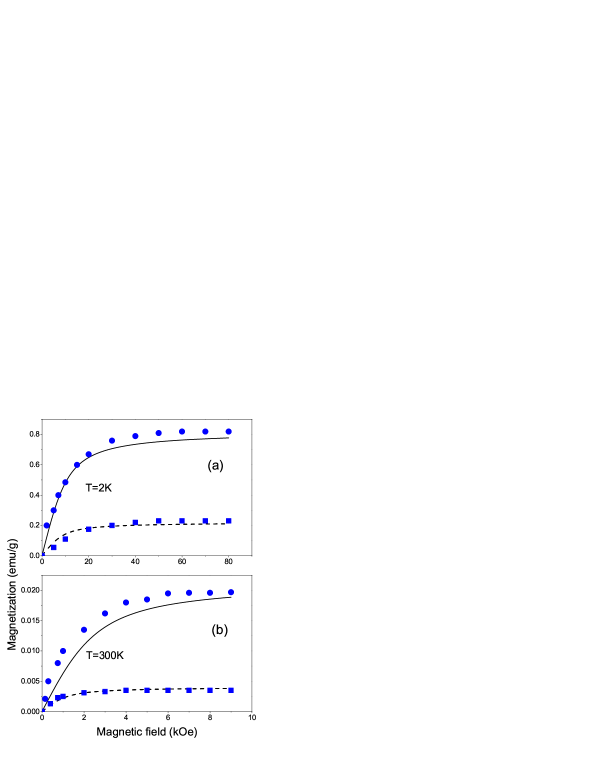
Figure 2: Magnetization curves of the defective graphene calculated with Eq. (13) (solid and dashed lines). Experimental data are taken from Ref. Wang09, for the samples Gr600 (circles) and Gr400 (squares) for T=2 K (a) and T=300 K (b). Fitting to the Gr600 data provides the $x=0.19$ and mean sizes of the domains $L=43$ nm ($T=2$ K, $T_{AF}=58$ K) and $L=1.6$ $\mu$m ($T=300$ K, $T_{AF}=1.5$ K); respectively $x=0.12$, $L=130$ nm ($T=2$ K, $T_{AF}=18$ K) and $L=5.6$ $\mu$m ($T=300$ K, $T_{AF}=0.5$ K) have been applied to Gr400.

References

- (1) M. Daghofer, N. Zheng, and A. Moreo, Phys. Rev. B 82, 121405(R) (2010).
- (2) T. G. Rappoport, M. Godoy, B. Uchoa, R. R dos Santos, and A. H. Castro Neto, arXive:1008.3189v1.
- (3) R. Balog, B. Jørgensen, L. Nilsson, M. Andersen, E. Rienks, M. Bianchi, M. Fanetti, E. Lægsgaard, A. Baraldi, S. Lizzit, Z. Sljivancanin, F. Besenbacher, B. Hammer, T. G. Pedersen, P. Hofmann, and L. Hornekær, Nature Mat. 9, 315 (2010).
- (4) W. Han, K. Pi, K. M. McCreary, Y. Li, J. J. I. Wong, A. G. Swartz, and R. K. Kawakami, Phys. Rev. Lett. 105, 167202 (2010).
- (5) N. Tombros, C. Jozsa, M. Popinciuc, H. T. Jonkman, and B. J. van Wees, Nature 448, 571 (2007).
- (6) P. Esquinazi, D. Spemann, R. Höhne, A. Setzer, K.-H. Han, and T. Butz, Phys. Rev. Lett. 91, 227201 (2003).
- (7) Y. Wang, Y. Huang, Y. Song, X. Zhang, Y. Ma, J. Liang, and Y. Chen, Nano Lett. 9, 220 (2009).
- (8) H. S. S. R. Matte, K. S. Subrahmanyam, and C. N. R. Rao, J. Phys. Chem. C 113, 9982 (2009).
- (9) M. Sepioni, R. R. Nair, S. Rablen, J. Narajanan, F. Tuna, R. Winpenny, A. K. Geim, and I. V. Grigorieva, Phys. Rev. Lett. 105, 207205 (2010).
- (10) O. V. Yazyev and M. I. Katsnelson, Phys. Rev. Lett. 100, 047209 (2008).
- (11) J. Červenka, M. I. Katsnelson, and C. F. J. Flipse, Nature Phys. 5, 840 (2009).
- (12) H.-H. Lin, T. Hikihara, H.-T. Jeng, B.-L. Huang, C.-Y. Mou, and X. Hu, Phys. Rev. B 79, 035405 (2009).
- (13) O. V. Yazyev and L. Helm, Phys. Rev. B 75, 125408 (2007).
- (14) H. Kumazaki and D. S. Hirashima, J. Phys. Soc. Jpn. 76, 064713 (2007)
- (15) L. Pisani, B. Montanari, and N. Harrison, New J. Phys. 10, 033002 (2008).
- (16) J. J. Palacios, J. Fernández-Rossier, and L. Brey, Phys. Rev. B 77, 195428 (R)(2008).
- (17) O. V. Yazyev, Rep. Prog. Phys. 73, 05650 (2010).
- (18) M. Hentschel and F. Guinea, Phys. Rev. B 76, 115407 (2007).
- (19) Z.-G. Zhu, K.-H. Ding, and J. Berakdar, Eur. Phys. Lett. 90, 67001 (2010).
- (20) J.-H. Chen, W. G. Cullen, E. D. Williams, and M. S. Fuhrer, arXiv_1004.3373.
- (21) B. Uchoa, T. G. Rappoport, and A. H. Castro Neto, arXive:1006.2512v1.
- (22) L. Brey, H. A. Fertig, and S. Das Sarma, Phys. Rev. Lett. 99, 116802 (2007).
- (23) V. V. Cheianov, Eur. Phys. J. Special Topics 148, 55 (2007).
- (24) T. G. Rappoport, B. Uchoa, and A. H. Castro Neto, Phys. Rev. B 80, 245408 (2009).
- (25) P. Venezuela, R. B. Muniz, A. T. Costa, D. M. Edwards, S. R. Power, and M. S. Ferreira, Phys. Rev. B 80, 241413(R) (2009).
- (26) A. M. Black-Schaffer, Phys. Rev. B 81, 205416 (2010).
- (27) E. H. Lieb, Phys. Rev. Lett. 62, 1201 (1989).
- (28) P. Esquinazi, J.Barzola-Quiquia, D. Spemann, M. Rothermel, H. Ohldag, N.García, A. Setzer, and T. Butz, J. Magn. Magn. Mat. 322, 1156 (2010).
- (29) M. P. López-Sancho , F. de Juan, and M. A. H. Vozmediano, J. Magn. Magn. Mat. 322, 1167 (2010).
- (30) N. D. Mermin and H. Wagner, Phys. Rev. Lett. 17, 1133 (1966).
- (31) D. Huertas-Hernando, F. Guennea, and A. Brataas, Phys. Rev. B 74, 155426 (2006).
- (32) A. H. Castro Neto, F. Guinea, N. M. R. Peres, K. S. Novoselov, and A. K. Geim, Rev. Mod. Phys. 81, 109 (2009).
- (33) E. M. Lifshitz and L. P. Pitaevskii, Statistical physics (Pergamon, Oxford, 1980), Part 2.
- (34) R. Englman, The Jahn-Teller Effect in Molecules and Crystals (Wiley, New York, 1972).
- (35) H. Bednarski, J. Magn. Magn. Mat. 213, 377 (2000).