Advanced Three Level Approximation for Numerical Treatment of Cosmological Recombination

Abstract

New public numerical code for fast calculations of the cosmological recombination of primordial hydrogen-helium plasma is presented. The code is based on the three-level approximation (TLA) model of recombination and allows us to take into account some fine physical effects of cosmological recombination simultaneously with using fudge factors. The code can be found at http://www.ioffe.ru/astro/QC/CMBR/atlant/atlant.html

1 Introduction

Cosmological recombination is one of the key processes in the early Universe. It determines the epoch of decoupling of radiation from matter and thereby determines the epochs at which baryonic matter can start to fall into gravitational potential wells created by clustering cold dark matter (CDM). Afterwards these CDM+baryonic matter clouds develop into non-relativistic gravity bound systems like galaxies (Peebles (1965, 1968); Doroshkevich et al. (1967); Ma & Bertschinger (1995)). The sizes of these proto-objects also depend on cosmological recombination via the kinetics of divergence of radiation and matter temperatures which determines the critical Jeans length. Cosmological recombination affects primordial chemistry (Dalgarno & Lepp (1987)) and correspondingly rate of radiative cooling of collapsing clouds (via emission in resonant lines of molecules which depends on the abundances of primordial molecules).

From observational point of view the cosmological recombination is also very important process because its kinetics determines the position of last scattering surface (Sunyaev & Zeldovich (1970), Hu et al. (1995)). This in turn affects the cosmic microwave background radiation (CMBR) anisotropy which is one of the main sources of information about evolution of the early Universe, its composition and other properties. A great number of experiments on CMBR anisotropy have been carried out in the last thirty years (Relikt-1 1983, COBE 1989, QMAP-Toco 1996, BOOMERanG 1997-2003, MAXIMA 1998-1999, WMAP 2001-present day, and many others). Treatment of the results of these experiments demands clear understanding of cosmological recombination physics. That is why many efforts have been made for theoretical investigation of cosmological recombination and development of applied numerical codes for modelling of this process (e.g. Zeldovich et al. (1968), Peebles (1968), Matsuda et al. (1969), Jones & Wyse (1985), Grachev & Dubrovich (1991), Seager et al. (1999)). Increasing accuracy of experiments in the last decade leads to increase of efforts of theorists in the study of details of cosmological recombination (see e.g. Dubrovich & Grachev (2005), Chluba et al. (2007); Chluba et al. (2010) Chluba & Sunyaev (2009a, 2010b), Rubiño-Martín et al. (2008), Switzer & Hirata (2008b), Hirata & Switzer (2008), Ali-Haïmoud et al. (2010)) and perfection of numerical codes. In the light of soon releases of experimental data from Planck mission this task becomes more and more important and urgent (for overview of efforts of investigators to find exact recombination scenario and to estimate remain uncertainties see e.g. Sunyaev & Chluba (2009); Shaw & Chluba (2011)). Today for successful treatment of Planck data the minimal required accuracy of numerical codes evaluating cosmological recombination is about 0.1% (on free electron fraction) for the epoch of hydrogen recombination and 1% for the epoch of helium recombination. Desirable accuracy is about 0.01% and 0.1% correspondingly.

The next possible step of the investigations of the early Universe in the epochs $z=800-10^{4}$ is the experimental study of CMBR spectral distortions originated from cosmological recombination of hydrogen and helium. Such experiments would be powerful sources of information about history of the Universe in these epochs. Thanks to the numerous theoretical works in this field (Dubrovich (1975), Lyubarsky & Sunyaev (1983); Fahr & Loch (1991); Rybicki & dell’Antonio (1993); Boschan & Biltzinger (1998); Dubrovich & Grachev (2004); Rubiño-Martín et al. (2008) and references therein) one can understand parameters of these spectral distortions clearly enough. Of course the cosmological recombination is an integral part of modelling of these distortions. Note that some simple methods for this problem (Bernshtein et al. (1977); Burgin (2003)) demand the knowledge of derivatives of ionization fractions of hydrogen and helium, so calculated ionization fractions should be smooth as possible (i.e. without sharp numerical features). In spite of the fact that detection of CMBR spectral distortions by cosmological recombination is impossible today, the rapid progress of measurement equipment for CMBR anisotropy allows us to hope that such experiments will be possible in the near future.

Thus the main aim of this work is to present numerical code covering investigations of cosmological recombination widely as possible within simple model which we used. Our code called atlant (advanced three level approximation for numerical treatment of cosmological recombination) may be useful for regular calculations of free electron fraction for treatment of CMBR anisotropy data, further investigations of cosmological recombination, theoretical predictions of new observational cosmological effects (e.g. Dubrovich et al. (2009); Grachev & Dubrovich (2010)), and comparison with other numerical codes (e.g. recfast by Seager et al. (1999) and Wong et al. (2008), RICO by Fendt et al. (2009), RecSparse by Grin & Hirata (2010), HyRec by Ali-Haïmoud & Hirata (2010a), CosmoRec by Chluba & Thomas (2010)).

2 Cosmological model

The standard cosmological model is used. Hubble constant $H$ as a function of redshift $z$ is given by the following equation:

$$H(z)=H_{0}\sqrt{\Omega_{\Lambda}+\Omega_{K}(1+z)^{2}+\Omega_{m}(1+z)^{3}+\Omega_{rel}(1+z)^{4}}$$ (1)

where $H_{0}$ is the value of Hubble constant in present epoch, $\Omega_{\Lambda}$ is the vacuum-like energy density, $\Omega_{K}$ is the energy density related to the curvature of the Universe, $\Omega_{m}$ is the energy density of non-relativistic matter, which includes contributions from CDM and baryonic matter $\Omega_{m}=\Omega_{CDM}+\Omega_{b}$. $\Omega_{rel}$ is the energy density of relativistic matter, which includes contributions from photons (mainly CMBR) and neutrinos $\Omega_{rel}=\Omega_{\gamma}+\Omega_{\nu}$.

The photon energy density is related to the temperature of CMBR:

$$\Omega_{\gamma}={a_{R}T_{0}^{4}\over\rho_{c}c^{2}}$$ (2)

where $a_{R}$ is the radiation constant, $T_{0}$ is the CMBR temperature at present epoch, $\rho_{c}=3H_{0}^{2}/\left(8\pi G\right)$ is the critical density of the Universe, $c$ is the speed of light, $G$ is the gravitational constant.

At the present epoch the relativistic neutrino energy density is related with the photon energy density by the following formula:

$$\Omega_{\nu}={7\over 8}N_{\nu}\left({4\over 11}\right)^{4/3}\Omega_{\gamma}$$ (3)

where $N_{\nu}$ is the effective number of neutrino types.

In this paper (and current version of code) we consider $\Omega_{tot}=\Omega_{\Lambda}+\Omega_{K}+\Omega_{m}+\Omega_{rel}=1$, so $\Omega_{K}$ is fixed by relation $\Omega_{K}=1-\left(\Omega_{\Lambda}+\Omega_{m}+\Omega_{rel}\right)$.

The total concentrations of hydrogen and helium depend on redshift by the following formulas:

$$N_{H}=N_{H0}\left(1+z\right)^{3}\;,\leavevmode\nobreak\ \leavevmode\nobreak\ \leavevmode\nobreak\ N_{He}=N_{He0}\left(1+z\right)^{3}$$ (4)

where $N_{H0}$ and $N_{He0}$ are the values of concentrations at present epoch. The total concentration of the primordial hydrogen atoms and ions at present epoch is given by the following relation:

$$N_{H0}={\rho_{c}\over m_{H}}\Omega_{b}X_{p}$$ (5)

where $m_{H}$ is the hydrogen atom mass, $X_{p}$ is the primordial hydrogen mass fraction (i.e. hydrogen mass fraction after the primordial nucleosynthesis).

The total concentration of the primordial helium atoms and ions at present epoch is given by the following relation:

$$N_{He0}={\rho_{c}\over m_{He}}\Omega_{b}Y_{p}$$ (6)

where $m_{He}$ is the helium atom mass, $Y_{p}=\left(1-X_{p}\right)$ is the primordial helium mass fraction. Fractions of other elements are considered negligible.

The temperature $T$ of equilibrium radiation background depends on redshift according to:

$$T=T_{0}\left(1+z\right)$$ (7)

3 Hydrogen Recombination

3.1 Main equations

The time-dependent behaviour of hydrogen ionization fraction in the isotropic homogeneous expanding Universe is described by the following kinetic equation (Zeldovich et al. (1968); Peebles (1968)):

$$\dot{x}_{HII}=-C_{HI}[\alpha_{HII}\left(T_{m}\right)N_{e}x_{HII}-\beta_{HI}\left(T\right)\exp\left(-{h\nu_{\alpha}\over k_{B}T}\right)x_{HI}]$$ (8)

where $x_{HII}=N_{HII}/\left(N_{H}+N_{He}\right)$, $C_{HI}$ is the factor by which the ordinary recombination rate is inhibited by the presence of HI Ly$\alpha$ resonance-line radiation, $\alpha_{HII}$ is the total HII$\rightarrow$HI recombination coefficient to the excited states of HI, $N_{e}=x_{e}N_{H}$ is the free electron concentration ($x_{e}$ is the free electron fraction in common notation, see e.g. recfast), $\beta_{HI}$ is the total HI$\rightarrow$HII ionization coefficient from the excited states of HI, $\nu_{\alpha}$ is the Ly$\alpha$ transition frequency, $T_{m}$ is the kinetic temperature of the electron gas, $x_{HI}=N_{HI}/\left(N_{H}+N_{He}\right)$ is the neutral hydrogen fraction. Note that ionization fractions of ionic components are defined relative to the total number of hydrogen and helium atoms and ions $\left(N_{H}+N_{He}\right)$ while free electron fraction $x_{e}$ is normalized to the concentration of hydrogen atoms and ions, $N_{H}$, as it is accepted commonly (so it is necessary for possible use of atlant results by other numerical codes).

The specific form of inhibition coefficient depends on fine effects which are taken into account. In the current version (1.0) of the code only radiative feedbacks for resonant transitions are taken into account from the whole list of known (considered until now) fine effects. Other fine effects are planned to be included in future works. So, the inhibition coefficient is given by the formula:

$$C_{HI}={A^{r}_{eff}+A_{2s1s}\over\beta_{HI}+A^{r}_{eff}+A_{2s1s}}$$ (9)

where $A^{r}_{eff}$ is the total effective coefficient of np$\leftrightarrow$1s transitions, $A_{2s1s}=8.22458$ s^-1 is the coefficient of 2s$\rightarrow$1s two-photon spontaneous transition (e.g. Goldman (1989)).

The recombination coefficient $\alpha_{HII}$ is given by the following approximation:

$$\alpha_{HII}\left(T\right)=F_{H}{aT_{4}^{b}\over 1+cT_{4}^{d}}$$ (10)

where $F_{H}$ is the hydrogen fudge factor by Seager et al. (1999), $T_{4}=T[K]/10^{4}$, and $a=4.309\cdot 10^{-13}$cm³s^-1, $b=-0.6166$, $c=0.6703$, $d=0.5300$ are the parameters fitted by Pequignot et al. (1991).

The ionization coefficient $\beta_{HI}$ can be found by using principle of detailed balance:

$$\beta_{HI}\left(T\right)=\alpha_{HII}\left(T\right)g_{e}\left(T\right)\exp\left({-{h\nu_{c2}\over k_{B}T}}\right)$$ (11)

where $g_{e}\left(T\right)={(2\pi m_{e}k_{B}T)^{3/2}/h^{3}}$ is the partition function of free electrons, $\nu_{c2}$ is the HI c$\rightarrow$2 transition frequency (here symbol “c” denotes continuum state).

Note that recombination and ionization coefficients included in the kinetic equation (8) should be calculated at different temperatures (see e.g. Ali-Haïmoud & Hirata (2010a)). Since the kinetics of recombination process is determined by the free electron distribution function, the recombination coefficient depends on kinetic temperature of free electrons $T_{m}$. The kinetics of ionization is determined by the photon distribution function, therefore ionization coefficient depends on temperature of photons $T$. Thus the detailed balance does not take place in considered case, and relation (11) has mathematical sense only and allows us to avoid direct calculation of ionization coefficient, $\beta_{HI}\left(T\right)$, from integral of collisions for photons and hydrogen atoms. Also exponential term in ionization part of (8), $\exp\left(-{h\nu_{\alpha}/\left[k_{B}T\right]}\right)$, should be calculated at the temperature of radiation. The distinction of temperatures used for calculation of ionization coefficients in the present code and in recfast (Seager et al. (1999); Wong et al. (2008), there the temperature of matter is used for this aim) leads to a little but important difference in the free electron fraction (see Fig. 1).

The equation (8) is solved numerically together with other main kinetic equations (19), (35) by using second-order method of integration of ODE system. The relative deviation between results obtained by atlant and recfast for the period of hydrogen cosmological recombination is presented in Fig. 1.

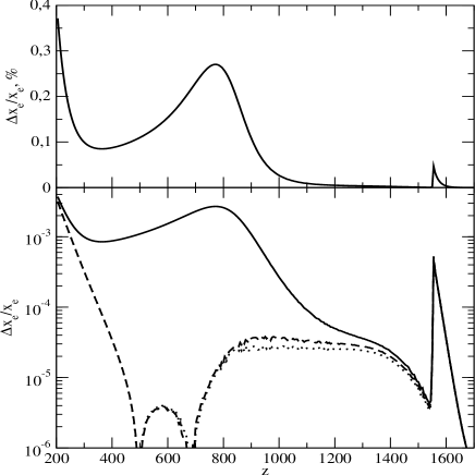
Figure 1: Top panel: the relative difference $\Delta x_{e}/x_{e}$ between free electron fractions calculated by atlant and recfast for the period of hydrogen recombination. Bottom panel: (i) solid curve corresponds to the relative difference $\Delta x_{e}/x_{e}$ between free electron fractions calculated by atlant and recfast [i.e. the same as in the top panel but in logarithmic scale], (ii) dashed curve corresponds to the relative difference $\Delta x_{e}/x_{e}$ between free electron fractions calculated by atlant and recfast with corrected ionization rate [i.e. ionization coefficient $\beta_{HI}\left(T\right)$ and exponential term $\exp\left(-{h\nu_{\alpha}/\left[k_{B}T\right]}\right)$ in Eq. (8) of recfast are calculated at the temperature of radiation $T$], (iii) dotted curve corresponds to the relative difference $\Delta x_{e}/x_{e}$ between free electron fractions calculated by atlant with modified ionization rate [i.e. ionization coefficient $\beta_{HI}\left(T_{m}\right)$ and exponential term $\exp\left(-{h\nu_{\alpha}/\left[k_{B}T_{m}\right]}\right)$ in Eq. (8) of atlant are calculated at the temperature of matter $T_{m}$] and recfast. Dashed and dotted curves are partially overlapped.

3.2 Radiative Feedbacks

Due to a great number of fine effects the radiative feedbacks for resonant transitions have been chosen for including in the first published version of recombination code. It is because physics of this effect is clear (it is difficult to state this is true about many other fine effects) and independently obtained results of calculation of this effect (Chluba & Sunyaev (2010a); Kholupenko et al. (2010)) confirm each other. Inclusion of feedbacks into the code is based on formulas suggested by Kholupenko et al. (2010). According this the total effective coefficient of np$\leftrightarrow$1s transitions is:

$$A^{r}_{eff}={8\pi H\nu_{\alpha}^{3}\over N_{HI}c^{3}}\delta_{A}$$ (12)

where $\delta_{A}$ is given by the following expression

$$\delta_{A}=\sum_{n\geq 2}^{n_{max}}C_{n}{\nu_{n}^{3}\over\nu_{\alpha}^{3}}\exp\left(-{E_{n}-E_{2}\over k_{B}T}\right)$$ (13)

where $\nu_{n}$ is the frequency of $n\rightarrow 1$ transition ($\nu_{2}=\nu_{\alpha}$), $E_{n}=h\nu_{n}$, and coefficients $C_{n}$ are:

$$C_{n}=\left(1-\Gamma_{H}(z^{\prime}_{n})/\Gamma_{H}(z)\right)$$ (14)

where in turn $\Gamma_{H}$ is the relative overheating of Ly$\alpha$ radiation (occupation number $\eta_{\alpha}$) in comparison with its equilibrium value (occupation number $\eta^{0}_{\alpha}$):

$$\Gamma_{H}=\left({\eta_{\alpha}/\eta^{0}_{\alpha}}-1\right)$$ (15)

and

$$z^{\prime}_{n}=\left((1+z){\nu_{n+1}/\nu_{n}}-1\right)$$ (16)

The set of formulas (12-16) allows us to calculate ionization history taking into account the feedbacks for hydrogen $n\rightarrow 1$ resonant transitions with principal quantum numbers $n\leq n_{max}$. For taking into account the feedback effect we use simple perturbation theory: at the first stage (unperturbed equations) atlant calculates the relative overheating $\Gamma_{H}$ and stores this, at the second stage atlant solves equations perturbed by the feedback effect. Relative deviation of free electron fraction between perturbed ($n_{max}=10$) and unperturbed calculations is presented in Fig. 2.

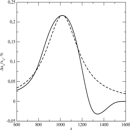
Figure 2: Dashed line corresponds to the relative difference between atlant with fudge function $\delta_{X}$ and base result [i.e. $\Delta x_{e}/x_{e}=\delta_{X}$]. Parameters of fudge function are the following: $A_{p}=2.166\cdot 10^{-3}$, $z_{p}=1019$, $\Delta z_{p}=180$. For comparison: solid line corresponds to the relative difference between feedback result for $n_{\rm max}=10$ [i.e. feedbacks $11\Rightarrow...\Rightarrow 2$ are taken into account] and the base result [i.e. without feedbacks].

3.3 Fudge factors

Developed recombination code allows users to use fudge factors as well as add physical effects. This opportunity has been included because of the following reasons: 1) list of fine effects leading to 0.01 - 0.1 % corrections in the ionization fraction may be incomplete, and it is difficult to say how long this list will be in final form and when this will be achieved; 2) considerations of some fine effects give contradictory results due to not completely clear physical picture (e.g. two-photon transitions from high excited states [Wong & Scott (2008), Hirata (2008), and Labzowsky et al. (2009)], recoil [Grachev & Dubrovich (2008) and Hirata & Forbes (2009)] and others).

First fudge factor is the common (see recfast) hydrogen fudge factor $F_{H}$ introduced in the expression (10) for hydrogen recombination coefficient $\alpha_{HII}$.

Second fudge factor is the perturbation function $\delta_{X}$ modifying free electron fraction:

$$x_{e}^{res}=x_{e}^{calc}\left(1+\delta_{X}\right)$$ (17)

where $x_{e}^{res}$ is the free electron fraction (normalized by the total concentration of hydrogen atoms and ions) being the final result of code running (i.e. it is value shown in the resulting file), $x_{e}^{calc}$ is the solution of ODE’s system describing ionization fractions and free electron fraction.

Note that function $\delta_{X}$ affects final result $x_{e}$ but not ODE’s system. This allows user to control changes of free electron fraction strictly by including fudge factors.

Analyzing previous works devoted to the fine effects of cosmological recombination (e.g. Grachev & Dubrovich (2008); Chluba & Sunyaev (2009b)) one may note that typical form of corrections to the ionization fraction can be described by a bell-shaped function (e.g. Lorentzian or Gaussian profile or others). In this work the Lorentzian function has been chosen to describe uncertain deviations (until now) of free electron fraction from well known ODE’s solution:

$$\delta_{X}={A_{p}\over 1+\left[\left(z-z_{p}\right)/\Delta z_{p}\right]^{2}}$$ (18)

where $A_{p}$ is the relative amplitude of perturbation of ionization fraction, $z_{p}$ is the redshift of perturbation maximum, $\Delta z_{p}$ is the half-width of perturbation function at half-altitude.

Result of use of fudge function is shown in the Fig. 2 where we have plotted $\Delta x_{e}/x_{e}=\delta_{X}$ as function of redshift $z$. Here we show how fudge function can mimic real fine corrections by means of example of feedback correction for $n_{max}=10$.

4 HeII$\rightarrow$HeI helium recombination

The time-dependent behaviour of HeII fraction in the isotropic homogeneous expanding Universe is described by the following kinetic equation (Kholupenko et al. (2007); Wong et al. (2008)):

$$\dot{x}_{HeII}=-C_{par}[\alpha_{par}N_{e}x_{HeII}-{g_{a}\over g_{g}}\beta_{par}\exp{\left(-{E_{ag}\over k_{B}T}\right)}x_{HeI}]$$

$$-C_{or}[\alpha_{or}N_{e}x_{HeII}-{g_{a^{\prime}}\over g_{g}}\beta_{or}\exp{\left(-{E_{a^{\prime}g}\over k_{B}T}\right)}x_{HeI}]$$ (19)

where $x_{HeII}=N_{HeII}/\left(N_{H}+N_{He}\right)$ is the fraction of HeII ions relative to the total number of hydrogen and helium atoms and ions, $C_{par}$ is the factor by which the ordinary recombination rate is inhibited by the presence of HeI $2^{1}p\rightarrow 1^{1}s$ resonance-line radiation, $\alpha_{par}$ is the total HeII$\rightarrow$HeI recombination coefficient to the excited para-states of HeI, subscript $a$ denotes $2^{1}s$ state of HeI atom, $N_{e}$ is the free electron concentration, $g_{a}=1$ is the statistical weight of $2^{1}s$ state of HeI, $g_{g}=1$ is the statistical weight of $1^{1}s$ state of HeI, $\beta_{par}$ is the total HeI$\rightarrow$HeII ionization coefficient from the excited para-states of HeI, $E_{ag}$ is the $2^{1}s\rightarrow 1^{1}s$ transition energy, $C_{or}$ is the factor by which the ordinary recombination rate is inhibited by the presence of HeI $2^{3}p\rightarrow 1^{1}s$ resonance-line radiation, $\alpha_{or}$ is the total HeII$\rightarrow$HeI recombination coefficient to the excited ortho-states of HeI, subscript $a^{\prime}$ denotes state $2^{3}s$ of HeI atom $g_{a^{\prime}}=3$ is the statistical weight of $2^{3}s$ state of HeI, $\beta_{or}$ is the total HeI$\rightarrow$HeII ionization coefficient from the excited ortho-states of HeI, $E_{a^{\prime}g}$ is the $2^{3}s\rightarrow 1^{1}s$ transition energy, $x_{HeI}=N_{HeI}/\left(N_{H}+N_{He}\right)$ is the neutral helium fraction.

The para- and ortho- recombination coefficients are given by widely used approximation formulas (e.g. Verner & Ferland (1996)) parameters of which are based on data by Hummer & Storey (1998)):

$$\alpha_{S}\left(T\right)=q_{S}\left({T\over T_{2}}\right)^{-1/2}\left(1+{T\over T_{2}}\right)^{-(1-p_{S})}\left(1+{T\over T_{1}}\right)^{-(1+p_{S})}$$ (20)

where subscript $S$ takes values ‘par’ or ‘or’, and $q_{S}$, $p_{S}$, $T_{1}=10^{5.114}$ K, $T_{2}=3$ K (Seager et al. (1999)) are the parameters of approximation. For the recombination via para-states we have $q_{par}=10^{-10.744}$cm³s^-1, $p_{par}=0.711$ (Seager et al. (1999)). For the recombination via ortho-states we have $q_{or}=10^{-10.306}$cm³s^-1, $p_{or}=0.761$ (Wong et al. (2008)).

The para- and ortho- recombination and ionization coefficients are related by the following formula

$$\beta_{S}={g_{c}\over g_{S}}\alpha_{S}g_{e}(T)\exp\left({-{E_{S}\over k_{B}T}}\right),$$ (21)

where subscript $``c^{\prime\prime}$ denotes continuum state of HeI atom, $g_{c}=4$ is the statistical weight of continuum state of (He⁺+e^-), $E_{par}$ is the $c\rightarrow 2^{1}s$ transition energy, $E_{or}$ is the $c\rightarrow 2^{3}s$ transition energy.

The inhibition factor $C_{par}$ is given by the following expression:

$$C_{par}={\left(g_{b}/g_{a}\right)A_{bg}P_{bg}\exp\left(-{E_{ba}/k_{B}T}\right)+A_{ag}\over\beta_{par}+\left(g_{b}/g_{a}\right)A_{bg}P_{bg}\exp\left(-{E_{ba}/k_{B}T}\right)+A_{ag}}$$ (22)

where $A_{bg}$ is the Einstein coefficient [s^-1] of $2^{1}p\leftrightarrow 1^{1}s$ spontaneous transitions, $P_{bg}$ is the probability of the uncompensated $2^{1}p\rightarrow 1^{1}s$ transitions, $E_{ba}$ is the $2^{1}p\rightarrow 2^{1}s$ transition energy, $A_{ag}$ is the coefficient of two-photon $2^{1}s\rightarrow 1^{1}s$ spontaneous decay.

The inhibition factor $C_{or}$ is given by the following expression

$$C_{or}={\left(g_{b^{\prime}}/g_{a^{\prime}}\right)A_{b^{\prime}g}P_{b^{\prime}g}\exp\left(-{E_{b^{\prime}a^{\prime}}/k_{B}T}\right)\over\beta_{or}+\left(g_{b^{\prime}}/g_{a^{\prime}}\right)A_{b^{\prime}g}P_{b^{\prime}g}\exp\left(-{E_{b^{\prime}a^{\prime}}/k_{B}T}\right)}$$ (23)

where subscript $b^{\prime}$ denotes state $2^{3}p$ of HeI, $g_{b^{\prime}}=9$ is the statistical weight of $2^{3}p$ state of HeI, where $A_{bg}$ is the Einstein coefficient [s^-1] of $2^{3}p\leftrightarrow 1^{1}s$ spontaneous transitions, $P_{b^{\prime}g}$ is the probability of the uncompensated $2^{3}p\rightarrow 1^{1}s$ transitions, $E_{b^{\prime}a^{\prime}}$ is the $2^{3}p\rightarrow 2^{3}s$ transition energy.

The probabilities $P_{bg}$ and $P_{b^{\prime}g}$ take into account the escape of HeI resonant photons from the line profiles due to the cosmological expansion and destruction of these photons by neutral hydrogen. They can be found by the following formula:

$$P_{fg}=P^{r}_{fg}+P^{H}_{fg}$$ (24)

where $P^{r}_{fg}$ is approximately given by the following:

$$P^{r}_{fg}=\left(1+\gamma^{-1}\right)^{-2}\tau_{He,f}^{-1}\left(1-\exp\left(-\tau_{He,f}\right)\right)$$ (25)

where $\gamma$ is the ratio of the helium and hydrogen absorption coefficients at the central frequency of the $f\rightarrow g$ line (here symbol $f=b$ or $b^{\prime}$ depending on what transition is considered), $\tau_{He,f}$ is the Sobolev optical depth. The value $\gamma$ is given by the following relation:

$$\gamma={\left(g_{f}/g_{g}\right)A_{fg}N_{HeI}c^{2}\over\sigma_{H}\left(\nu_{fg}\right)8\pi^{3/2}\nu_{fg}^{2}\Delta\nu_{D,f}N_{HI}}$$ (26)

where $\sigma_{H}$ is the ionization cross-section of hydrogen ground state, parameter $\Delta\nu_{D,f}=\nu_{fg}\sqrt{2k_{B}T/\left(m_{He}c^{2}\right)}$ is the Doppler line width.

Table 1: Parameters of the approximation of $P^{H}_{D}$

Range of $\gamma$	p	q
$0\leq\gamma\leq 5\cdot 10^{2}$	0.66	0.9
$5\cdot 10^{2}<\gamma\leq 5\cdot 10^{4}$	0.515	0.94
$5\cdot 10^{4}<\gamma\leq 5\cdot 10^{5}$	0.416	0.96
$5\cdot 10^{5}<\gamma$	0.36	0.97

The optical depth $\tau_{He,f}$ is:

$$\tau_{He,f}={g_{f}A_{fg}N_{HeI}c^{3}/\left(g_{g}8\pi H\nu_{fg}^{3}\right)}$$ (27)

The value $P^{H}_{fg}$ is given by the following:

$$P^{H}_{fg}=P^{H}_{D}+P^{H}_{G}+P^{H}_{R}$$ (28)

where in turn $P^{H}_{D}$ approximately is:

$$P^{H}_{D}=\left(1+p\gamma^{q}\right)^{-1}$$ (29)

where parameters $p$, $q$ are given in the Tab. LABEL:tab_pq.

The value $P^{H}_{G}$ is given by the following approximate formula:

$$P^{H}_{G}=(8\lambda a)^{1/4}\pi^{-5/8}\gamma^{-3/4}\cdot$$

$$\cdot\left[1+\exp\left(-1.07\ln\left(s+1.5\right)-0.45\right)\right]\left(s+1.28\right)^{-1/2}$$ (30)

where $a=\Gamma_{f}/4\pi\Delta\nu_{D,f}$ is the Voigt parameter (here $\Gamma_{f}$ is the natural line width), $\lambda$ is the single-scattering albedo in $f\rightarrow g$ line, and parameter $s$ is given by the following relation (Grachev (1988)):

$$s=2^{-3/2}\pi^{-1/4}(1-\lambda)\lambda^{-1/2}a^{1/2}\gamma^{1/2}-1/4$$ (31)

The single-scattering albedo $\lambda$ can be calculated by:

$$\lambda\simeq{A_{fg}\over A_{fg}+R_{f}}$$ (32)

where $R_{f}=\sum_{n}R_{f\rightarrow n}$ is the total coefficient of radiative transitions (including induced transitions, while collision transitions are considered negligible) from $f$ state to excited states of HeI atom.

The value $P^{H}_{R}$ is approximately:

$$P^{H}_{R}=2(1-\lambda)\sqrt{a\over(1-\lambda)\gamma\pi^{3/2}}\left({\pi\over 2}-\arctan\left(f(a,\lambda,\gamma)\right)\right)$$ (33)

where $f(a,\lambda,\gamma)$ is defined by the expression

$$f(a,\lambda,\gamma)\simeq 0.69\cdot(1-\lambda)^{-1/2}\lambda^{1/4}\left(a\gamma\right)^{-1/4}\sqrt{\ln{\gamma}}$$ (34)

The equation (19) is solved numerically together with other main kinetic equations (8) and (35) to determine free electron fraction $x_{e}$. The relative deviation of free electron fraction between the results calculated by using atlant and recfast for the period of HeII$\rightarrow$HeI recombination is presented in Fig. 3.

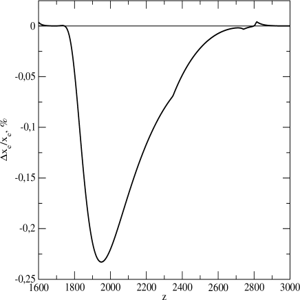
Figure 3: The relative difference $\Delta x_{e}/x_{e}$ between free electron fractions calculated by atlant and recfast for the period of HeII$\rightarrow$HeI recombination.

5 HeIII$\rightarrow$HeII helium recombination

In the difference with recfast we use non-equilibrium (i.e. kinetic) approach for consideration of HeIII$\rightarrow$HeII helium recombination. The time-dependent behaviour HeIII fraction in the isotropic homogeneous expanding Universe is described by the following kinetic equation:

$$\dot{x}_{HeIII}=-C_{HeII}[\alpha_{HeIII}N_{e}x_{HeIII}-$$

$$\beta_{HeII}\exp\left(-{h\nu_{HeII,21}\over k_{B}T}\right)x_{HeII}]$$ (35)

where $x_{HeIII}=N_{HeIII}/\left(N_{H}+N_{He}\right)$, $C_{HeII}$ is the factor by which the ordinary recombination rate is inhibited by the presence of HeII $2p\rightarrow 1s$ resonance-line radiation, $\alpha_{HeIII}$ is the total HeIII$\rightarrow$HeII recombination coefficient to the excited states of HeII, $\beta_{HeII}$ is the total HeII$\rightarrow$HeIII ionization coefficient from the excited states of HeII, $\nu_{HeII,21}$ is the HeII $2p\rightarrow 1s$ transition frequency.

The inhibition coefficient is given by the expression:

$$C_{HeII}={A^{r}_{HeII,2p1s}+A_{HeII,2s1s}\over\beta_{HeII}+A^{r}_{HeII,2p1s}+A_{HeII,2s1s}}$$ (36)

where $A^{r}_{HeII,2p1s}$ is the effective coefficient of HeII 2p$\leftrightarrow$1s transitions, $A_{HeII,2s1s}$ is the coefficient of HeII 2s$\rightarrow$1s two-photon spontaneous transition.

Since HeII is the hydrogenic ion the recombination coefficient $\alpha_{HeIII}$ can be found by using simple scaling relation (see e.g. Verner & Ferland (1996)):

$$\alpha_{Z}\left(T\right)=Z\alpha_{1}\left(T/Z^{2}\right)$$ (37)

where $Z$ is the nuclear charge for the hydrogenic ions. In considered case Eq. (37) yields $\alpha_{HeIII}\left(T\right)=2\alpha_{HII}\left(T/4\right)$, where $\alpha_{HII}$ is taken from (10) without hydrogen fudge factor $F_{H}$.

The ionization coefficient $\beta_{HeII}$ can be found by using principle of detailed balance:

$$\beta_{HeII}\left(T\right)=\alpha_{HeIII}\left(T\right)g_{e}\left(T\right)\exp\left({-{h\nu_{HeII,c2}\over k_{B}T}}\right)$$ (38)

$\nu_{HeII,c2}$ is the HeII c$\rightarrow$2 transition frequency.

Note that in Eq (35) the recombination and ionization coefficients are calculating at the same temperature $T$. This is because the matter temperature $T_{m}$ is very close to the radiation one $T$ (relative deviation is less than $10^{-5}$) during HeIII$\rightarrow$HeII recombination and calculation at different temperatures has no sense at required level of accuracy.

The effective coefficient $A^{r}_{HeII,2p1s}$ of HeII 2p$\leftrightarrow$1s transitions due to escape of HeII 2p$\leftrightarrow$1s resonant photons from the line profile because of cosmological redshift is given by the following formula:

$$A^{r}_{HeII,2p1s}={8\pi H\nu_{HeII,21}^{3}\over N_{HeII}c^{3}}$$ (39)

The value $A_{HeII,2s1s}$ is found from charge scaling for the hydrogenic ions $A_{Z,2s1s}=Z^{6}A_{2s1s}$ (see e.g. Shapiro & Breit (1959), Zon & Rapoport (1968), Nussbaumer & Schmutz (1984)). In the considered case this gives us $A_{HeII,2s1s}=2^{6}A_{2s1s}$.

The equation (35) is solved numerically together with other main kinetic equations (8) and (19) to determine free electron fraction $x_{e}$. The relative deviation between results by atlant and recfast for the period of HeIII$\rightarrow$HeII recombination is presented in Fig. 4.

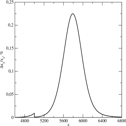
Figure 4: The relative difference $\Delta x_{e}/x_{e}$ between free electron fractions calculated by atlant and recfast for the period of HeIII$\rightarrow$HeII recombination.

6 Evolution of matter temperature

The behaviour of the matter temperature in the isotropic homogeneous expanding Universe is described by the following equation (e.g. Peebles (1968); Scott & Moss (2009)):

$$\dot{T}_{m}={8\sigma_{T}a_{R}T^{4}\over 3m_{e}c}{x_{e}\over 1+x_{e}+N_{He0}/N_{H0}}\left(T-T_{m}\right)-2HT_{m}$$ (40)

where $\sigma_{T}$ is the Thomson scattering cross section.

Defining relative deviation, $\delta_{T}$, of the matter temperature from the radiation temperature via $T_{m}=T\left(1-\delta_{T}\right)$ and substituting this into (40) one can obtain:

$$\dot{\delta}_{T}=-\left(R_{T}+H\right)\delta_{T}+H$$ (41)

where $R_{T}$ is the rate of energy transfer between matter and radiation via Compton scattering:

$$R_{T}={8\sigma_{T}a_{R}T^{4}\over 3m_{e}c}{x_{e}\over 1+x_{e}+N_{He0}/N_{H0}}$$ (42)

To solve equation (41) we applied a perturbation approach. In the early stages of the Universe history ($z\gtrsim 200$) the rate of energy transfer between matter and radiation via Compton scattering is much larger than the rate of the temperature change (the latter is about Hubble expansion rate $H$), i.e. $\dot{\delta}_{T}/\left(R_{T}\delta_{T}\right)\ll 1$. Thus we can use expansion of the solution over this smallness:

$$\delta_{T}=\sum_{i=0}^{\infty}\delta_{T,i}$$ (43)

where zeroth-order approximation is determined as quasistacionary solution of Eq. (41) (see also Hirata (2008); Ali-Haïmoud & Hirata (2010b)):

$$\delta_{T,0}=\left(R_{T}/H+1\right)^{-1}$$ (44)

and the next members of expansion (43) are related by the following equation:

$$\delta_{T,i+1}=-\left(R_{T}+H\right)^{-1}\dot{\delta}_{T,i}$$ (45)

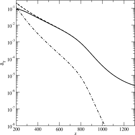
Figure 5: The corrections, $\delta_{T}$, to the matter temperature, $T_{m}$, relative to the radiation temperature, $T$, as functions of redshift $z$: dashed curve corresponds to the correction, $\delta_{T,0}$, dashed-dotted curve corresponds to $|\delta_{T,1}|$ ($\delta_{T,1}<0$), and solid curve corresponds to $\left(\delta_{T,0}+\delta_{T,1}\right)$.

In the present version of the code we keep only two first corrections $\delta_{T,0}$ and $\delta_{T,1}$ in Eq. (43).

For the period $z\lesssim 200$ the quasistationary condition is violated, so expansion (43) loses convergence and cannot represent the solution of Eq. (41). In this redshift range we use the following dependence of matter temperature on redshift:

$$T_{m}=T_{m}^{dec}\left({1+z\over 1+z_{dec}}\right)^{2}$$ (46)

where $T_{m}^{dec}$ is the matter temperature from (43) at $z_{dec}$ (index “dec” means “decoupling”) which is considered as the moment of decoupling of the matter temperature from radiation the one (at value $z_{dec}$ we should make join of solutions). In present version of code we determine $z_{dec}$ from condition $\delta_{T,0}=0.5$. Equation (46) corresponds to the equation of state of non-relativistic matter.

Results of calculations of $\delta_{T,0}$ and $\delta_{T,1}$ are presented in Fig. 5. The influence of taking into account different approximations for $\delta_{T}$ [depending on the number of kept members of expansion (43)] on the free electron fraction is shown in Fig. 6.

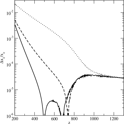
Figure 6: The relative difference $\Delta x_{e}/x_{e}$ of the free electron fractions as a function of redshift $z$: dotted curve corresponds to the difference, $\Delta x_{e}/x_{e}$, between results for $\delta_{T}=0$ (i.e. $T_{m}=T$) by atlant and recfast corrected (for the details of corrections, see section 3.1 of the present paper), dashed curve corresponds to the difference, $\Delta x_{e}/x_{e}$, between results for $\delta_{T}=\delta_{T,0}$ by atlant and corrected recfast, and solid curve corresponds to the difference, $\Delta x_{e}/x_{e}$, between results for $\delta_{T}=\left(\delta_{T,0}+\delta_{T,1}\right)$ by atlant and corrected recfast.

7 Variation of the fundamental constants

Today the opportunity to vary of the fundamental constants becomes essential at the analysis of CMBR anisotropy (e.g. Scóccola et al. (2008)) and we decided to include this in our code. Thus the current version of the code allows user to see how recombination occurs at different values of the fundamental constants (this means that changes of fundamental constants lead to corresponding changes of derived physical values, e.g. ionization energies of atoms, Thomson cross section and others).

Since some of used physical values are given only numerically (e.g. level energies and transition probabilities for HeI atom, see www.nist.gov) we use simple scalings to take into account the influence of variation of fundamental constants on these values. These scalings are the following:
1) For the level energies:

$$E=E_{st}\left({e\over e_{st}}\right)^{4}\left({m_{e}\over m_{e,st}}\right)\left({\hbar\over\hbar_{st}}\right)^{-2}$$ (47)

2) For the one-photon transition coefficients:

$$A^{\gamma}=A^{\gamma}_{st}\left({e\over e_{st}}\right)^{10}\left({m_{e}\over m_{e,st}}\right)\left({\hbar\over\hbar_{st}}\right)^{-6}\left({c\over c_{st}}\right)^{-3}$$ (48)

3) For the two-photon transition coefficients:

$$A^{\gamma\gamma}=A^{\gamma\gamma}_{st}\left({e\over e_{st}}\right)^{16}\left({m_{e}\over m_{e,st}}\right)\left({\hbar\over\hbar_{st}}\right)^{-9}\left({c\over c_{st}}\right)^{-6}$$ (49)

4) For the recombination coefficients:

$$\alpha=\alpha_{st}\left({e\over e_{st}}\right)^{6}\left({m_{e}\over m_{e,st}}\right)^{-3/2}\left({\hbar\over\hbar_{st}}\right)^{-1}\left({c\over c_{st}}\right)^{-3}$$ (50)

In the expressions (47)-(50) subscript “st” denotes current values of physical quantities while symbols without subscript denote values which user suggests to be valid during the recombination epoch.

The influence of variations of the fine structure constant $\alpha_{fine}$ (via varying elementary charge) on the free electron fraction is shown in Fig. 7.

Figure 7: Free electron fractions $x_{e}$ as functions of redshift $z$ at different values of the fine-structure constant $\alpha_{fine}$: dashed curve corresponds to $\alpha_{fine}/\alpha^{0}_{fine}=0.95$, solid curve corresponds to $\alpha_{fine}/\alpha^{0}_{fine}=1$, dashed-dotted curve corresponds to $\alpha_{fine}/\alpha^{0}_{fine}=1.05$

8 Results

The main numerical results of this paper are the relative differences of free electron fractions $\Delta x_{e}/x_{e}$ calculated by atlant and recfast (figs 1, 3, 4). In the top panel of Fig. 1 the relative difference $\Delta x_{e}/x_{e}$ between result of atlant and current version of recfast (version 1.5, Wong et al. (2008)) for the hydrogen recombination epoch. The first significant difference appears in the period $z=1550-1650$. This is because at early epochs $z\gtrsim 1550$ recfast considers recombination as quasi-equilibrium process (according to Saha formula) and sets initial condition for the kinetic equation correspondingly, while atlant considers recombination as a non-equilibrium (kinetic) process in the whole range of redshifts and sets an initial conditions corresponding to the fully ionized plasma at the moment given by user (in our case $z_{begin}=8000$). The sharp peak of $\Delta x_{e}/x_{e}$ in the period $z=1550-1650$ (maximal value is about $5\cdot 10^{-4}$) is due to transition from recombination according to Saha formula to non-equilibrium recombination which occurs in recfast at free electron fraction $x_{e}=0.985$ (that corresponds to $z\simeq 1555$ in considered case). There is a simple method of modelling of CMBR spectral distortion due to cosmological recombination (e.g. Bernshtein et al. (1977); Dubrovich & Stolyarov (1995, 1997); Burgin (2003)). This method is based on the formalism of matrix of efficiency of radiative transitions (ERT-matrix) and it does not demand direct calculation of atomic level populations. On the other hand this method demands use of the following values $dx_{HII}/dz$, $dx_{HeII}/dz$, and $dx_{HeIII}/dz$ to determine the rates of resonance photon emission and correspondingly the shape of cosmological recombination lines. Thus for using ERT-matrix method the sharp numerical features may be significant defects of cosmological recombination modelling. The second difference of results by atlant and recfast appears in the period $z=300-1000$. It arises due to different structure of ionization items of hydrogen kinetic equation (8) in atlant and recfast: in recfast the ionization coefficient $\beta_{HI}$ and Boltzmann exponential term are calculated at the temperature of matter while in atlant at the radiation temperature. Most part of this difference is due to distinction of ionization coefficients including in the denominator of inhibition coefficient $C_{HI}$. The maximum of $\Delta x_{e}/x_{e}$ in mentioned range of redshifts is about 0.27% at $z\simeq 770$. This is little but maybe important difference in the context of future analysis of Planck data. The third difference appears at low redshifts ($z\lesssim 300$). It is due to the different approaches to evaluating matter temperature in recfast (where ODE for temperature is solved) and in atlant (where perturbation theory for temperature estimate is used). In the bottom panel of Fig. 1 we present three curves. Solid curve is the same as in the top panel but in a logarithmic scale. Dashed curve corresponds to the relative difference $\Delta x_{e}/x_{e}$ between free electron fractions calculated by atlant and recfast with corrected ionization rate [i.e. ionization coefficient $\beta_{HI}\left(T\right)$ and exponential term $\exp\left(-{h\nu_{\alpha}/\left[k_{B}T\right]}\right)$ in Eq. (8) of the recfast model are calculated at the temperature of radiation, $T$]. Dotted curve corresponds to the relative difference $\Delta x_{e}/x_{e}$ between free electron fractions calculated by atlant with modified ionization rate [i.e. ionization coefficient $\beta_{HI}\left(T_{m}\right)$ and exponential term $\exp\left(-{h\nu_{\alpha}/\left[k_{B}T_{m}\right]}\right)$ in Eq. (8) of the atlant model are calculated at the temperature of matter $T_{m}$] and recfast. These curves show that in the frame of identical physical models the accordance of results by atlant and recfast is wholly satisfactory. Residual difference which does not exceed $5\cdot 10^{-5}$ for the period $z=400-1500$ can be explained by a little different values of physical constants and different integration methods which have been used in atlant and recfast.

In Fig. 2 we demonstrate how feedbacks for resonant transitions of hydrogen affect free electron fraction (solid curve) and show an example of using fudge function, $\delta_{X}$ (dashed curve). The change due to feedbacks has the maximum about 0.2166% at redshift $z\simeq 1019$ in full accordance with Chluba & Sunyaev (2010a). This calculation has been done for $n_{max}=10$. Parameters of the fudge function have been choosen as following: $A_{p}=2.166\cdot 10^{-3}$, $z_{p}=1019$, and $\Delta z_{p}=180$. This is to show how use of the fudge function allows us to imitate the influence of real physical effects on the free electron fraction.

In Fig. 3 the relative difference of the results by atlant and recfast for the epoch of HeII$\rightarrow$HeI recombination is presented. The breaks in the range $z=2700-2900$ and break at $z\simeq 2300$ are the numerical features connected with switch in recfast code. The maximum of difference is about -0.23% at $z\simeq 1950$. The difference between results by atlant and recfast for the epoch of HeII$\rightarrow$HeI recombination arises because different approximations for estimate of effective eacape probability are used: in atlant the approach based on analytical consideration of resonance radiation transfer in the presence of continuum absorption is used (Kholupenko et al. (2008)) while recfast uses the simple approximation with an additional fudge factor $b_{He}$ (Wong et al. (2008)). It leads to the numerical differences because used approximations are not identical. Also there is physical reason for divergence of these approximations: Wong et al. (2008) have determined $b_{He}$ from the best agreement with result by Switzer & Hirata (2008a) who took into account not only hydrogen continuum opacity but also feedbacks for resonant transitions of HeI and found this effect is about 0.46% at $z\simeq 2045$. Later works (e.g. Chluba & Sunyaev (2010a)) show that this feedback effect is about 0.17% at $z\simeq 2300$, i.e. negligible for the most of modern problems connected with cosmological recombination (e.g. CMBR anisotropy analysis). Thus we do not take helium feedbacks into account in the present version of the code. One more important point of calculations of effective escape probability for HeI is the estimate of number of neutral hydrogen at the high redshifts $z\gtrsim 1600$ (i.e. when hydrogen ionization fraction close to unity [e.g. greater than 0.985]): recfast uses Saha formula for this aim, while in atlant the kinetic equation is solved in the whole range of redshifts to determine the fractions of all considered plasma components. This explains the discrepancy between results of the present paper and Kholupenko et al. (2008) where approximation by Wong et al. (2008) has also been investigated by using earlier version of our code (i.e. Wong-Moss-Scott approximation has been calculated, but number of neutral hydrogen has been calculated from kinetic equation).

In Fig. 4 the relative difference of the results by atlant and recfast for the epoch of HeIII$\rightarrow$HeII recombination is presented. The break at $z=5000$ is the numerical feature connected with switches in recfast code again. In the range of redshifts $z=5000-7000$ the difference between the results by atlant and recfast arises because HeIII$\rightarrow$HeII recombination is treated by atlant in non-equilibrium way while recfast treats this according to Saha formula. The maximum of difference is about 0.225% at $z\simeq 5790$. Such difference is too small to be a reason of any observational effects at the current level of experimental accuracy, but non-equilibrium treatment of HeIII$\rightarrow$HeII allows us to avoid artificial numerical features (that is important for the modelling of CMBR spectral distortion arising from HeIII$\rightarrow$HeII recombination).

In Fig. 5 the deviation of the matter temperature from the radiation temperature is presented. The dashed curve corresponds to the correction $\delta_{T,0}$, dashed-dotted curve corresponds to $|\delta_{T,1}|$, and solid curve corresponds to $\left(\delta_{T,0}+\delta_{T,1}\right)$. One can see that difference between the radiation and matter temperature is less than $10^{-4}$ down to $z\simeq 940$ and less than $10^{-3}$ down to $z\simeq 790$. Taking into account that $T_{m}$ is included in kinetic equation (8) only via recombination coefficient $\alpha_{HII}\left(T_{m}\right)$ one can expect the similar changes in hydrogen ionization fraction at transition from approximation $T_{m}=T$ to more exact estimate of $T_{m}$. From accuracy point of view the correction $\delta_{T,1}$ becomes important beginning from $z\simeq 480$ where/when it achieves values about $10^{-3}$. At the low $z$ ($z\lesssim 300$) the correction $\delta_{T,1}$ is larger than 20% of $\delta_{T,0}$ and should be taken into account for correct determination of residual ionization fraction as possible. In Fig. 6 we show how including of $\delta_{T,i}$’s affects the free electron fraction. We have compared our results with the results by recfast corrected in the following way: ionization items of Eq. (8), i.e. ionization coefficient $\beta_{HI}$ and exponential term $\exp\left(-{h\nu_{\alpha}/\left[k_{B}T_{m}\right]}\right)$ are calculated at temperature of radiation $T$. The dotted curve corresponds to the relative difference $\Delta x_{e}/x_{e}$ of the result by atlant for approximation $T_{m}=T$ (i.e. $\delta_{T}=0$) and the mentioned result by recfast, the dashed one corresponds to $\Delta x_{e}/x_{e}$ at $\delta_{T}=\delta_{T,0}$, and the solid one does $\Delta x_{e}/x_{e}$ at $\delta_{T}=\left(\delta_{T,0}+\delta_{T,1}\right)$. From Fig. 6 one can see that rough approximation $T_{m}=T$ is quite valid (at required level of accuracy) down to $z\simeq 670$ where $\Delta x_{e}/x_{e}$ achieves values about $10^{-3}$. Thus using this rough approximation biases the results not so dramatically as it seems when this approximation is used in recfast. More advanced approximations are valid ($\Delta x_{e}/x_{e}\leq 10^{-3}$) down to $z\simeq 310$ ($\delta_{T}=\delta_{T,0}$) and $z\simeq 250$ ($\delta_{T}=\left(\delta_{T,0}+\delta_{T,1}\right)$).

Fig. 7 illustrates one of the additional opportunities of atlant: here the changes of free electron fraction at variation of the fine-structure constant are presented. Presented results are obtained for the following values of the fine-structure constant $\alpha_{fine}$: $0.95\alpha^{0}_{fine}$, $\alpha^{0}_{fine}$, and $1.05\alpha^{0}_{fine}$ (where $\alpha^{0}_{fine}$ is the current value of the fine-structure constant). Obtained results are very similar to the results by Scóccola et al. (2008).

Acknowledgements Authors are grateful to participants of Workshops “Physics of Cosmological Recombination” (Max Planck Institute for Astrophysics, Garching 2008 and University Paris-Sud XI, Orsay 2009) for useful discussions on cosmological recombination.

This work has been partially supported by Ministry of Education and Science of Russian Federation (contract # 11.G34.31.0001 with SPbSPU and leading scientist G.G. Pavlov), RFBR grant 11-02-01018a, and grant “Leading Scientific Schools of Russia” NSh-3769.2010.2. Balashev S. A. also thanks the Dynasty Foundation.

References

- Ali-Haïmoud et al. (2010) Ali-Haïmoud Y., Grin D., Hirata C. M., 2010, Phys. Rev. D, 82, 123502
- Ali-Haïmoud & Hirata (2010a) Ali-Haïmoud Y., Hirata C. M., 2010a, arxiv:1011.3758
- Ali-Haïmoud & Hirata (2010b) Ali-Haïmoud Y., Hirata C. M., 2010b, Phys. Rev. D, 82, 063521
- Bernshtein et al. (1977) Bernshtein I. N., Bernshtein D. N., Dubrovich V. K., 1977, Soviet Astronomy, 21, 409
- Boschan & Biltzinger (1998) Boschan P., Biltzinger P., 1998, A&A, 336, 1
- Burgin (2003) Burgin M. S., 2003, Astronomy Reports, 47, 709
- Chluba et al. (2007) Chluba J., Rubiño-Martín J. A., Sunyaev R. A., 2007, MNRAS, 374, 1310
- Chluba & Sunyaev (2008b) Chluba J., Sunyaev R. A., 2008b, A&A, 480, 629
- Chluba & Sunyaev (2009a) Chluba J., Sunyaev R. A., 2009a, A&A, 503, 345
- Chluba & Sunyaev (2009b) Chluba J., Sunyaev R. A., 2009b, A&A, 496, 619
- Chluba & Sunyaev (2010a) Chluba J., Sunyaev R. A., 2010a, MNRAS, 402, 1221
- Chluba & Sunyaev (2010b) Chluba J., Sunyaev R. A., 2010b, A&A, 512, A53+
- Chluba & Thomas (2010) Chluba J., Thomas R. M., 2010, MNRAS, pp 1876–+
- Chluba et al. (2010) Chluba J., Vasil G. M., Dursi L. J., 2010, MNRAS, 407, 599
- Dalgarno & Lepp (1987) Dalgarno A., Lepp S., 1987, Astrochemistry, IAU Symposium, 120, 109
- Doroshkevich et al. (1967) Doroshkevich A. G., Zeldovich Y. B., Novikov I. D., 1967, Soviet Astronomy, 11, 233
- Dubrovich (1975) Dubrovich V. K., 1975, Soviet Astronomy Letters, 1, 196
- Dubrovich & Grachev (2004) Dubrovich V. K., Grachev S. I., 2004, Astronomy Letters, 30, 657
- Dubrovich & Grachev (2005) Dubrovich V. K., Grachev S. I., 2005, Astronomy Letters, 31, 359
- Dubrovich et al. (2009) Dubrovich V. K., Grachev S. I., Romanyuk V. G., 2009, Astronomy Letters, 35, 723
- Dubrovich & Stolyarov (1995) Dubrovich V. K., Stolyarov V. A., 1995, A&A, 302, 635
- Dubrovich & Stolyarov (1997) Dubrovich V. K., Stolyarov V. A., 1997, Astronomy Letters, 23, 565
- Fahr & Loch (1991) Fahr H. J., Loch R., 1991, A&A, 246, 1
- Fendt et al. (2009) Fendt W. A., Chluba J., Rubiño-Martín J. A., Wandelt B. D., 2009, ApJS, 181, 627
- Goldman (1989) Goldman S. P., 1989, Phys. Rev. A, 40, 1185
- Grachev (1988) Grachev S. I., 1988, Astrophysics, 28, 119
- Grachev & Dubrovich (1991) Grachev S. I., Dubrovich V. K., 1991, Astrophysics, 34, 124
- Grachev & Dubrovich (2008) Grachev S. I., Dubrovich V. K., 2008, Astronomy Letters, 34, 439
- Grachev & Dubrovich (2010) Grachev S. I., Dubrovich V. K., 2010, arxiv:1010.4455
- Grin & Hirata (2010) Grin D., Hirata C. M., 2010, Phys. Rev. D, 81, 083005
- Hirata (2008) Hirata C. M., 2008, Phys. Rev. D, 78, 023001
- Hirata & Forbes (2009) Hirata C. M., Forbes J., 2009, Phys. Rev. D, 80, 023001
- Hirata & Switzer (2008) Hirata C. M., Switzer E. R., 2008, Phys. Rev. D, 77, 083007
- Hu et al. (1995) Hu W., Scott D., Sugiyama N., White M., 1995, Phys. Rev. D, 52, 5498
- Hummer & Storey (1998) Hummer D. G., Storey P. J., 1998, MNRAS, 297, 1073
- Jones & Wyse (1985) Jones B. J. T., Wyse R. F. G., 1985, A&A, 149, 144
- Kholupenko & Ivanchik (2006) Kholupenko E. E., Ivanchik A. V., 2006, Astronomy Letters, 32, 795
- Kholupenko et al. (2007) Kholupenko E. E., Ivanchik A. V., Varshalovich D. A., 2007, MNRAS, 378, L39
- Kholupenko et al. (2008) Kholupenko E. E., Ivanchik A. V., Varshalovich D. A., 2008, Astronomy Letters, 34, 725
- Kholupenko et al. (2010) Kholupenko E. E., Ivanchik A. V., Varshalovich D. A., 2010, Phys. Rev. D, 81, 083004
- Labzowsky et al. (2009) Labzowsky L., Solovyev D., Plunien G., 2009, Phys. Rev. A, 80, 062514
- Lyubarsky & Sunyaev (1983) Lyubarsky Y. E., Sunyaev R. A., 1983, A&A, 123, 171
- Ma & Bertschinger (1995) Ma C., Bertschinger E., 1995, ApJ, 455, 7
- Matsuda et al. (1969) Matsuda T., Satō H., Takeda H., 1969, Progress of Theoretical Physics, 42, 219
- Nussbaumer & Schmutz (1984) Nussbaumer H., Schmutz W., 1984, A&A, 138, 495
- Peebles (1965) Peebles P. J. E., 1965, ApJ, 142, 1317
- Peebles (1968) Peebles P. J. E., 1968, ApJ, 153, 1
- Pequignot et al. (1991) Pequignot D., Petitjean P., Boisson C., 1991, A&A, 251, 680
- Rubiño-Martín et al. (2008) Rubiño-Martín J. A., Chluba J., Sunyaev R. A., 2008, A&A, 485, 377
- Rybicki & dell’Antonio (1993) Rybicki G. B., dell’Antonio I. P., 1993, Observational Cosmology, Astronomical Society of the Pacific Conference Series, 51, 548
- Scóccola et al. (2008) Scóccola C. G., Landau S. J., Vucetich H., 2008, Physics Letters B, 669, 212
- Scott & Moss (2009) Scott D., Moss A., 2009, MNRAS, 397, 445
- Seager et al. (1999) Seager S., Sasselov D. D., Scott D., 1999, ApJ, 523, L1
- Seager et al. (2000) Seager S., Sasselov D. D., Scott D., 2000, ApJS, 128, 407
- Shapiro & Breit (1959) Shapiro J., Breit G., 1959, Phys. Rev., 113, 179
- Shaw & Chluba (2011) Shaw J. R., Chluba J., 2011, arxiv:1102.3683
- Sunyaev & Chluba (2009) Sunyaev R. A., Chluba J., 2009, Astronomische Nachrichten, 330, 657
- Sunyaev & Zeldovich (1970) Sunyaev R. A., Zeldovich Y. B., 1970, Astrophysics and Space Science, 7, 3
- Switzer & Hirata (2008a) Switzer E. R., Hirata C. M., 2008a, Phys. Rev. D, 77, 083006
- Switzer & Hirata (2008b) Switzer E. R., Hirata C. M., 2008b, Phys. Rev. D, 77, 083008
- Verner & Ferland (1996) Verner D. A., Ferland G. J., 1996, ApJS, 103, 467
- Wong & Scott ( 2008) Wong W. Y., Scott D., 2007, MNRAS, 375, 1441
- Wong et al. (2008) Wong W. Y., Moss A., Scott D., 2008, MNRAS, 386, 1023
- Zeldovich et al. (1968) Zeldovich Y. B., Kurt V. G., Syunyaev R. A., 1968, Zhurnal Eksperimentalnoi i Teoreticheskoi Fiziki, 55, 278
- Zon & Rapoport (1968) Zon B. A., Rapoport L. P., 1968, Soviet Journal of Experimental and Theoretical Physics Letters, 7, 52