Pathogen evolution in switching environments: a hybrid dynamical system approach

Abstract

We propose a hybrid dynamical system approach to model the evolution of a pathogen that experiences different selective pressures according to a stochastic process. In every environment, the evolution of the pathogen is described by a version of the Fisher-Haldane-Wright equation while the switching between environments follows a Markov jump process. We investigate how the qualitative behavior of a simple single-host deterministic system changes when the stochastic switching process is added. In particular, we study the stability in probability of monomorphic equilibria. We prove that in a “constantly” fluctuating environment, the genotype with the highest mean fitness is asymptotically stable in probability while all others are unstable in probability. However, if the probability of host switching depends on the genotype composition of the population, polymorphism can be stably maintained.

Remark. This is a corrected version of the paper that appeared in Mathematical Biosciences 240 (2012), p. 70-75. A corrigendum has appeared in the same journal.

1 Introduction

Living organisms face changing environmental conditions. Parasites are a case in point: after each transmission event they find themselves in a new host that may be quite different from the previous one. For example, the immune system of the new host may respond differently to the parasite, and the new host may have a different genotype or even belong to a different species. Thus, a parasite genotype that is characterized by a high fitness in one host may have a low fitness in a different host. The question therefore arises how parasites evolve under the fluctuating selective pressures imposed on them through transmission events to different hosts.

Most of the studies so far have focused on models for host-pathogen interactions in a deterministic context [11, 12]. In some applications however it is natural to assume that environment (and hence fitness landscape) switching is not deterministic. For example, a pathogen could switch to a different host. Evolution of the pathogen then takes place in the new host (or environment), where the pathogen genotypes face different selective pressures, hence the dynamics of the pathogen genotypes are different. We remark that the evolving organism need not be a pathogen, nor is the environment necessarily a “host”.

Evolution of organisms in deterministically and randomly varying environments has been studied by many authors, see [2] for an early review. Karlin and collaborators [5, 6] introduced both deterministic and stochastic models for the evolution of haploid and diploid organisms under changing selection intensities for fixed and varying population sizes. In case of a deterministic two-allele model they showed that the genotype with higher selection intensity goes to fixation and the time to fixation varies according to the selection intensities. Furthermore, they investigated a stochastic model where generational selection intensities are identically distributed independent random variables. They focused on the question how the probabilities of fixation and the times to fixation change in the stochastic model. In [7], Kirzhner et al. considered a 4-dimensional system of difference equations for the haplotype frequencies of a two-locus model. Typical two-locus models show either fixation in one or both loci or stable polymorphic cycles, with period equaling the period of the environmental changes, i.e. the periodic fitness values. They however showed the existence of so called supercycles that have 1100 times the period of the periodically changing environment. The questions of structural stability, i.e. sensitivity in terms of the fitness parameters and the size of the basin of attraction of these cycles were investigated. Similarly, Nagylaki [10] investigated the existence of genetic polymorphisms for two-allele models with periodically varying fitness values. He showed that in a continuous differential equation model genetic polymorphism will persist with periods equaling the periods of the varying fitness values, however in a discrete model fixation is also possible.

Hybrid switching differential equations and more generally hybrid switching diffusions have found many applications in wireless communications, queuing networks, ecology [15] and financial mathematics, to name but a few; see [14] and the references therein. The word “hybrid” refers to the coexistence of continuous dynamics and discrete events, see also the related concept of piecewise deterministic processes [1]. In this paper we study a simplified version of the continuous time Fisher-Haldane-Wright equation (also known as standard replicator equation, [3]) subject to fitnesses driven by a Markov jump process. It is well known that in the deterministic Fisher-Haldane-Wright model the pathogen genotype that has the highest fitness value will go to fixation. The coupling of different Fisher-Haldane-Wright equations by a Markov process however requires a new definition of the concept of “highest fitness”. Hence we study the possible changes to the stability behaviors of the monomorphic equilibrium states depending on the stationary distribution of the switching Markov process. First we establish analytical results for the stability/instability of equilibria in the hybrid model. We show that in the case of a state-independent switching process, the monomorphic equilibrium of the genotype with highest mean fitness is asymptotically stable in probability while the monomorphic equilibria of all other genotypes are unstable in probability. As the stationary distribution of the switching Markov process varies, so does the mean fitness of each genotype. This results in exchanges of stability without the merger of the equilibria during the transition process. We may call this a “stochastic transcritical bifurcation”. Finally, we present some numerical simulations to illustrate our result and also an example of a state-dependent switching process.

2 The switching differential equation

We consider a model for $m$ genotypes of a pathogen evolving in $n$ possible environments. Let $w^{k}_{i}>0$ denote the fitness value of genotype $i$ in environment $k$. We assume for simplicity that for any fixed environment $k$, the fitness values $w^{k}_{i}$ are all different. We write $\mathbf{w}_{i}$ for the vector of all fitness values of genotype $i$. Let $P_{i}$ denote the frequency of pathogen $i$, so that the dynamics in each environment takes place in the $(m-1)$-dimensional simplex

$$\mathbb{T}^{m-1}=\left\{P\in\mathbb{R}_{\geq 0}^{m}\>|\>\sum_{i=1}^{m}P_{i}=1\right\}.$$

We write $P(t)=(P_{1}(t),P_{2}(t),\dots,P_{m}(t))$ for the state of the system at time $t$. The frequency dynamics of pathogen genotype $i$ in environment $k$ is given by

$$\frac{dP_{i}(t)}{dt}=P_{i}(t)\left(w_{i}^{k}-\displaystyle\sum_{j=1}^{m}w^{k}_{j}P_{j}(t)\right)=:F_{i}(P(t),k).$$ (2.1)

This equation is the Fisher-Haldane-Wright equation for frequencies of genotypes of asexually proliferating organisms. The rate of growth or decay of a genotype is determined by the difference of its fitness and the average fitness of the population. Observe that the simplex $\mathbb{T}^{m-1}$ and any of its subsimplices are invariant under the dynamics given by equation (2.1). It can be shown by straightforward computation that the average fitness in environment $k$

$$\phi^{k}(P)=\sum_{i=1}^{m}w^{k}_{i}P_{i}$$ (2.2)

satisfies

$$\frac{d}{dt}\phi^{i}(P(t)) =\sum_{i=1}^{m}w^{k}_{i}P_{i}\left(w^{k}_{i}-\sum_{j=1}^{m}w^{k}_{j}P_{j}\right)=\sum_{i=1}^{m}P_{i}(w_{i}^{k})^{2}-\left(\sum_{i=1}^{m}P_{i}w_{i}^{k}\right)^{2}$$

$$=\sum_{i=1}^{m}P_{i}(w_{i}^{k})^{2}-2\left(\sum_{i=1}^{m}P_{i}w_{i}^{k}\right)^{2}+\sum_{i=1}^{m}\left(\sum_{j=1}^{m}P_{j}w_{j}^{k}\right)^{2}P_{i}$$

$$=\sum_{i=1}^{m}P_{i}\left(w^{k}_{i}-\sum_{j=1}^{m}w^{k}_{j}P_{j}\right)^{2}\geq 0,$$

with equality if and only if $P$ is an equilibrium. It follows from the global existence of solutions and LaSalle’s theorem that every trajectory of (2.1) approaches one of the finitely many equilibria situated at the vertices of the simplex, see [8].

The environment switches according to a continuous time stochastic process $\alpha(t)$ that takes values in the set $\mathcal{M}=\{1,2,\dots,n\}$. The switching process $\alpha$ is a Markov process with (possibly state-dependent) generator matrix $Q(P)$ whose entries $q_{kl}(P)$ are defined by

$$\mathbf{P}\{\alpha(t+\Delta t)=l\,|\,\alpha(t)=k,\,(P(s),\alpha(s)),\,s\leq t\}=q_{kl}(P(t))\Delta t+o(\Delta t).$$ (2.3)

The elements $q_{kl}$ of the generator matrix $Q$ satisfy $q_{kl}\geq 0$ for all $k\neq l$ and $\displaystyle\sum_{l\in\mathcal{M}}q_{kl}=0$ for every $k\in\mathcal{M}$ (such a matrix is said to have the $q$-property, see [13]). The complete hybrid switching ordinary differential equation can be cast in the form

$$\frac{dP}{dt} =F(P(t),\alpha(t)),$$ (2.4)

$$P(0) =p\in\mathbb{T}^{m-1},\quad\alpha(0)=\alpha\in\mathcal{M},\quad\text{a.~{}s.},$$

where $\alpha(t)=k$ determines the environment $k$ at time $t$ and $F=(F_{1},\dots,F_{m})$ are defined by (2.1). The right hand side of the differential equation in (2.4) is globally Lipschitz continuous on the compact set $\mathbb{T}^{m-1}\times\mathcal{M}$. This implies global existence and uniqueness of solutions in the sense of stochastic processes, see [14, Theorem 2.1].

For the equation (2.1) restricted to a fixed environment $k$, the vertices $e_{i}$ of the simplex $\mathbb{T}^{m-1}$ (i.e. the unit vectors of $\mathbb{R}^{m}$) are all the equilibrium solutions. It is easy to show that all but one of these equilibria are unstable and that the stable equilibrium in environment $k$ is the one for which the fitness value $w^{k}_{i}$ is the largest. In the following section we investigate how this result generalizes to the case that stochastic switching is introduced. For this of course, we need to first generalize the concept of stability to switching ordinary differential equations.

3 Stability and instability in probability

In this section we establish results concerning the stability and instability of monomorphic steady states of the hybrid model. We first recall the following definition [14, Definition 8.1].

Definition 3.1

Let $(X^{x,\alpha}(t))_{t\geq 0}$ be the solution of a hybrid switching ordinary differential equation

$$\dot{X}(t) =F(X(t),\alpha(t)),\quad$$

$$\mathbf{P}\{\alpha(t+\Delta t) =l\,|\,\alpha(t)=k,\,(X(s),\alpha(s)),\,s\leq t\}=q_{kl}(X(t))\Delta t+o(\Delta t),$$

$$X(0) =x,\quad\alpha(0)=\alpha\;\text{a.~{}s.},$$

and let (without loss of generality) $x=0$ be an equilibrium solution, i.e. a solution of the equation $F(0,\alpha)=0$ for every $\alpha\in\mathcal{M}$. We say that $0$ is stable in probability if

$$\lim_{x\to 0}\mathbf{P}\left\{\sup_{t\geq 0}|X^{x,\alpha}(t)|>r\right\}=0$$

for every $\alpha\in\mathcal{M}$ and every $r>0$. We say that $0$ is asymptotically stable in probability if it is stable in probability and

$$\lim_{x\to 0}\mathbf{P}\left\{\lim_{t\to\infty}X^{x,\alpha}(t)=0\right\}=1$$

for every $\alpha\in\mathcal{M}$. Finally, $0$ is unstable in probability if it is not stable in probability.

For $n$-tuples of functions $g(\,\cdot\,,k)\in C^{1}(\mathbb{R}^{m})$ one defines a linear operator $\mathcal{L}$, the stochastic Lie derivative (see [14, Equation (8.3), p. 219])

$$\mathcal{L}g(x,k)=F(x,k)\cdot\nabla g(x,k)+\sum_{l=1}^{n}q_{kl}(x)g(x,k),$$

where $\nabla$ denotes the gradient with respect to the $x$-variable for fixed $k\in\mathcal{M}$. This is a natural generalization of the derivative of a scalar function along a vector field well known in the theory of ordinary differential equations. The following is Proposition 8.6, [14, p. 223].

Theorem 3.2

Let $D\subset\mathbb{R}^{m}$ be a neighborhood of $0$ and assume that there exists a function $V:D\times\mathcal{M}\to[0,\infty)$ with the following properties

• $V(\,\cdot\,,k)$ is continuous and vanishes only at $0$,

• $V(\,\cdot\,,k)$ is continuously differentiable in $D\setminus\{0\}$, and

• there exists a function $\kappa:(0,r)\to(0,\infty)$ such that for all $k\in\mathcal{M}$ and $|x|>\varrho$,

  $$\mathcal{L}V(x,k)\leq-\kappa(\varrho)<0.$$

Then the equilibrium $x=0$ is asymptotically stable in probability.

A function that satisfies the conditions of the theorem is called a Lyapunov function (for asymptotic stability).

Throughout the remainder of this section we consider the case of a state-independent generator matrix $Q$ with a universal stationary distribution $\pi=(q_{1},\dots,q_{n})$. This is the solution of the equations

$$\pi\cdot\mathbf{1}=1,\quad\textrm{and}\quad\pi Q=\mathbf{0}.$$

If $q_{kl}>0$ for all $k\neq l$ then the matrix $Q$ is irreducible and $\pi>0$ is unique [13, p. 21].

Theorem 3.3

Let $P_{1}$ be the genotype with the highest mean fitness, that is

$$\pi\cdot\mathbf{w}_{1}>\pi\cdot\mathbf{w}_{i}\quad\text{for all }\,i=2,\dots,m$$ (3.5)

Then the equilibrium $e_{1}$ is asymptotically stable in probability.

Remark 3.4   For almost every stationary distribution $\pi\in\mathbb{T}^{n-1}$, exactly one genotype satisfies a condition similar to (3.5).

Proof. For $i=2,\dots,m$ we set $a^{k}_{i,1}=w^{k}_{i}-w^{k}_{1}$ for the difference of fitness values with respect to genotype 1 and $\mathbf{a}_{i,1}=(a_{i,1}^{1},\dots,a_{i,1}^{n})$. Using the constraint $\displaystyle\sum_{j=1}^{m}P_{j}(t)=1$, we eliminate $P_{1}$ and obtain the reduced systems

$$\frac{dP_{i}(t)}{dt}=a_{i,1}^{k}P_{i}(1-P_{i})-P_{i}\sum_{j=2,\,j\neq i}^{m}a_{i,1}^{k}P_{j},$$

for $i=2,\dots,m$ and $k=1,\dots,n$. Notice that for fixed environment $k$ the linear part of this system has a diagonal structure. We define

$$\beta_{i}:=-\pi\cdot\mathbf{a}_{i,1}>0,$$

with the last inequality holding true since genotype 1 has the higher mean fitness compared to every other genotype. For $i=2,\dots,m$ we solve the systems of equations

$$Q\mathbf{c}_{i}=\mathbf{a}_{i,1}+\beta_{i}\mathbf{1}$$

for the vector $\mathbf{c}_{i}=(c_{i}^{1},\dots,c_{i}^{n})$ where $\mathbf{1}$ is the column vector with $n$ entries 1. The right hand sides of these equation are orthogonal to the kernel of $Q$ which is spanned by $\mathbf{1}$, hence there exist solutions. For $i=2,\dots,m$ and $k=1,\dots,n$, we define

$$V_{i}(P_{i},k)=(1-\gamma c_{i}^{k})P_{i}^{\gamma},\quad P_{i}>0,$$

with $0<\gamma<1$ yet to be selected, in such a way that all coefficients are positive. We have

$$\mathcal{L}V_{i}(P_{i},k) =\gamma(1-\gamma c_{i}^{k})P_{i}^{\gamma-1}(a_{i,1}^{k}P_{i}+o(1))+\sum_{j=1}^{n}q_{kj}(1-\gamma c_{i}^{j})P_{i}^{\gamma}$$ (3.6)

$$=\gamma P_{i}^{\gamma}\left((1-\gamma c_{i}^{k})a_{i,1}^{k}-\sum_{j=1}^{n}q_{kj}c_{i}^{j}+o(1)\right)$$

$$=\gamma P_{i}^{\gamma}\left((1-\gamma c_{i}^{k})a_{i,1}^{k}-(a_{i,1}^{k}+\beta_{i})+o(1)\right)$$

$$=\gamma P_{i}^{\gamma}\left(-\gamma c_{i}^{k}a_{i,1}^{k}+\pi\cdot\mathbf{a}_{i,1}+o(1)\right),$$

where we have made use of the fact that the row sums of $Q$ are zero. In order to make all the factors in parentheses negative, we have to choose $0<\gamma<1$ such that the inequality

$$\pi\cdot\mathbf{a}_{i,1}<\gamma c_{i}^{k}a_{i}^{k}$$ (3.7)

holds. By assumption (3.5), the left hand side of inequality (3.7) is negative. Therefore, for those indices $i$ and $k$ for which $c_{i}^{k}a_{i,1}^{k}\geq 0$, no condition arises for $\gamma$. If on the other hand $c_{i}^{k}a_{i,1}^{k}<0$, then we can select

$$0<\gamma<\min_{i=2,\dots m\atop k=1,\dots,n}\left\{\frac{\pi\cdot\mathbf{a}_{i,1}}{c_{i}^{k}a_{i,1}^{k}}\>:\>c_{i}^{k}a_{i,1}^{k}<0\right\}.$$

Although the $c_{i}^{k}$ are not explicitly known, this is a minimum of finitely many positive numbers. The Lyapunov function is the sum of functions of a single variable

$$V(P_{2},\dots,P_{m},k)=\sum_{i=2}^{m}V_{i}(P_{i},k)$$

and the condition of Proposition 8.6 in [14] follows from the linearity of the operator $\mathcal{L}$ and the choice of $\gamma$. $\Box$

Instability in probability of an equilibrium can be proved similarly. The following is Proposition 8.7, [14, p. 223]. Notice however that the Lyapunov function does not vanish but has a pole at the unstable equilibrium.

Theorem 3.5

Let $D\subset\mathbb{R}^{m}$ be a neighborhood of $0$ and assume that there exists a function $V:D\times\mathcal{M}\to[0,\infty)$ with the following properties

• $V(\,\cdot\,,k)$ is continuously differentiable in $D\setminus\{0\}$, and

• there exists a function $\kappa:(0,r)\to(0,\infty)$ such that for all $k\in\mathcal{M}$ and $|x|>\varrho$,

  $$\mathcal{L}V(x,k)\leq-\kappa(\varrho)<0,$$

• for all $k\in\mathcal{M}$,

  $$\lim_{|x|\to 0}V(x,k)=\infty.$$

Then the equilibrium $x=0$ is unstable in probability.

Theorem 3.6

Under the assumption (3.5) of Theorem 3.3, the equilibrium $e_{i},\,i=2,\dots,m$ is unstable in probability.

Proof. The proof is very similar to that of Theorem 3.3, so we only give a sketch here. This time it is $P_{i}$ that is being eliminated from the system containing $P_{1}$ and $P_{i}$. This results in the reduced systems

$$\frac{dP_{l}(t)}{dt}=a_{l,i}^{k}P_{l}(1-P_{l})-P_{l}\sum_{j\neq i,l}^{m}a_{j,i}^{k}P_{j},$$

for $l\neq i$ and $a^{k}_{l,i}=w^{k}_{l}-w^{k}_{i}$. For $i=2,\dots,m$ let $\mathbf{c}_{i}=(c_{i}^{1},\dots,c_{i}^{n})$ be the solution of

$$Q\mathbf{c}_{i}=\mathbf{a}_{1,i}-\beta_{i}\mathbf{1}.$$

We set

$$V(P_{1},\dots,P_{i-1},P_{i+1},\dots,P_{m},k)=V(P_{1},k)=(1-\gamma c_{i}^{k})P_{1}^{\gamma},\quad P_{1}>0,$$

where $0>\gamma>-1$ has yet to be selected, small enough that all coefficients are positive. With a calculation similar to (3.6) we obtain

$$\mathcal{L}V(P_{1},k) =\gamma(1-\gamma c_{i}^{k})P_{1}^{\gamma-1}(a_{1,i}^{k}P_{1}+o(1))+\sum_{j=1}^{n}q_{kj}(1-\gamma c_{i}^{j})P_{1}^{\gamma}$$

$$=\gamma P_{1}^{\gamma}\left((1-\gamma c_{i}^{k})a_{1,i}^{k}-\sum_{j=1}^{n}q_{kj}c_{i}^{j}+o(1)\right)$$

$$=\gamma P_{1}^{\gamma}\left((1-\gamma c_{i}^{k})a_{1,i}^{k}-(a_{1,i}^{k}-\beta_{i})+o(1)\right)$$

$$=\gamma P_{1}^{\gamma}\left(-\gamma c_{i}^{k}a_{1,i}^{k}+\pi\cdot\mathbf{a}_{1,i}+o(1)\right).$$

In order to make all the factors in parentheses positive (so that the entire expression becomes negative), we need to have

$$0>\gamma>\max_{i=2,\dots m\atop k=1,\dots,n}\left\{\frac{\pi\cdot\mathbf{a}_{1,i}}{c_{i}^{k}a_{1,i}^{k}}\>:\>c_{i}^{k}a_{1,i}^{k}<0\right\}.$$

The expressions whose maximum is taken are all negative since $\pi\cdot\mathbf{a}_{1,i}>0$ by assumption (3.5). The condition of Proposition 8.7 in [14] is thereby verified. $\Box$

Remark 3.7   The notion of “highest mean fitness” requires that the generator matrix $Q$ is independent of the state and so has a universal stationary distribution $\pi$. If $Q$ depends continuously on $P$, it is still possible to formulate the corresponding “local” stability results for the equilibria $e_{i}$ by taking $\pi$ to be a stationary distribution of $Q(e_{i})$.

4 Numerical simulations and examples

The following is an interesting example of how stability can arise through stochastic coupling. Let the fitness values of three genotypes in two environments be given by

$$w^{1}_{1}=1,\,w^{1}_{2}=\frac{7}{10},\,w^{1}_{3}=\frac{11}{10},$$

$$w^{2}_{1}=1,\,w^{2}_{2}=\frac{11}{10},\,w^{2}_{3}=\frac{7}{10}.$$

Although genotype 1 does not have the highest fitness in any environment, it has the highest mean fitness for stationary distributions $(q,1-q)$ with $\frac{1}{4}<q<\frac{3}{4}$, see Figure 1. If the generator matrix $Q$ of the Markov process does not depend explicitly on the state $P(t)$, we can determine the switching times a priori according to $t_{i+1}=t_{i}+\tau$, where $\tau$ is an exponentially distributed random variable with mean $1$ (for example).

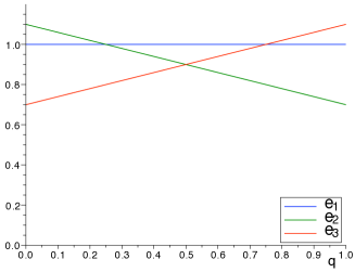
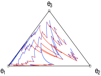
Figure 1: (Left panel) The mean fitness of the three equilibria as a function of the parameter $q$ of the stationary distribution. (Right panel) Trajectories converging to $e_{1}$ when $q=\frac{1}{2}$. Parts of the trajectory in red indicate that environment 1 is active (when $e_{3}$ is attracting) while parts of the trajectory in blue indicate that environment 2 is active (when $e_{2}$ is attracting).

To finish this section, we present two example with a state-dependent generator matrix $Q(P)$. Let $n=m=2$,

$$w^{1}_{1}=w^{2}_{2}=1,\>w^{1}_{2}=w^{2}_{1}=\frac{8}{10},\\$$

and define two switching matrix functions

$$Q_{1}(P_{1},P_{2}) =\begin{pmatrix}-P_{2}&P_{2}\\ P_{1}&-P_{1}\end{pmatrix},$$

$$Q_{2}(P_{1},P_{2}) =\begin{pmatrix}-P_{1}&P_{1}\\ P_{2}&-P_{2}\end{pmatrix}.$$

This choice of the generator matrix means that the jump process favors jumps into the environment that is beneficial (in case $Q_{1}$), respectively disadvantageous (in case $Q_{2}$) for the genotype that currently dominates. In contrast to the previous simulations with state-independent generator matrix, it is now necessary to update the transition matrix of the Markov chain, namely $\exp(Q(P)\Delta t)$ during each time step of length $\Delta t$. Following [14, Chapter 5.3], we use the approximation $I+Q(P)\Delta t$. The stationary distribution of $Q_{1}(e_{i})$ is, incidentally, $e_{i}$ for $i=1,2$. It follows from Theorem 3.3 and Remark 3 that both equilibria are locally asymptotically stable in probability. Conversely, the stationary distribution of $Q_{2}(e_{1})$ is $e_{2}$ and vice versa. Under this regime, both equilibria are locally unstable in probability. The results in Figure 2 show that stochastic bistability may arise (for the choice $Q_{1}(P)$, left panel) or that solutions do not converge to a monomorphic steady state (for the choice $Q_{2}(P)$, right panel).

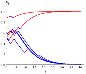
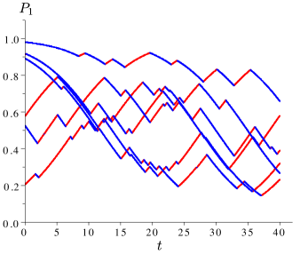
Figure 2: A state-dependent generator matrix $Q_{1}(P)$ leads to bistability (left panel) whereas matrix $Q_{2}(P)$ results in failure to converge to an equilibrium (right panel). Parts of the trajectory in red indicate that environment 1 is active (when $e_{1}$ is attracting) while parts of the trajectory in blue indicate that environment 2 is active (when $e_{2}$ is attracting).

In terms of biological interpretation, one can conceive of competing pathogen genotypes that cause different behaviors in the affected host. For example, if the dominating pathogen genotype has only mild effects on their host’s well-being, infected individuals may retain their usual mobility and thereby make a transition into a new environment more likely. On the other hand, if the dominating pathogen genotype causes severe morbidity, the host may exhibit restricted mobility so that a transition into a new environment becomes less likely.

5 Conclusions

In this work we consider the dynamics of a simple host-pathogen system, where pathogen genotype frequencies evolve according to a simple deterministic model. The selective pressures switch according to a Markov process. We use the framework of switching differential equations to compare the evolution of the pathogen in a single deterministic versus a hybrid system. In the switching system interesting new stability patterns emerge, depending on the stationary distribution of the underlying Markov process. We assume a fixed number of environments (and corresponding fitnesses), in contrast to previous works. For example, Karlin and collaborators [5, 6] assumed that the fitnesses during each generation are independent identically distributed random variables. Gillespie on the other hand in [4] proposed a stochastic differential equation where the fitness is a process with continuous sample paths.

In the case of a state-independent generator matrix of the Markov process $Q$, we have a partition of the simplex $\mathbb{T}^{n-1}$ of all possible stationary distributions $\pi$ into regions where one genotype has a greater mean fitness than all others, except for a set of measure zero where two genotypes have equal mean fitness (where bifurcations occur). This complete classification relies on the diagonal structure of the Jacobian of the reduced system (LABEL:reduced_systems) at the equilibrium $0$. Due to this decoupling, it is possible to use a sum of Lyapunov functions that all depend on one variable only. In this way, we obtain a condition for asymptotic stability using convex combinations of corresponding elements of the spectra of the Jacobians in the different environments. We expect such a result to hold in the greater context of switching ordinary differential equations and diffusion processes with regime switching.

Our work can be refined and extended in various ways. Firstly, we use a very simple deterministic competition model (2.1), where the pathogen genotypes are ordered according to their fitness values and the only equilibria are the vertices of the simplex $\mathbb{T}^{m-1}$. A straightforward extension would be to consider the continuous time Fisher-Haldane-Wright equation for diploid organisms for which there exist equilibria in the interior of $\mathbb{T}^{m-1}$. Other competition models may lead to deterministic bistability or to periodic orbits (for example the rock-paper-scissors game [3]). Secondly, although the host switching process is stochastic, we model within-host evolution in a deterministic way. A more realistic approach would incorporate random genetic drift into the model. This may be particularly important during transmission events, which often involve population bottlenecks due to small inoculum sizes. Finally, our model only considers a single chain of transmission events and neglects between-host selection as well as superinfections. It may be possible to also consider multiple (branching and coalescing) transmission chains and thus fully couple within-host and epidemiological dynamics [9].

References

- [1] E. Buckwar and M. G. Riedler, An exact stochastic hybrid model of excitable membranes including spatio-temporal evolution, J. Math. Biol. 63 (2011), 1051-1093.
- [2] J. Felsenstein, The theoretical population genetics of variable selection and migration, Ann. Rev. Genet. 10 (1976), 253-280.
- [3] E. Frey, Evolutionary game theory: Theoretical concepts and applications to microbial communities, Physica A 389 (2010), 4365-4298.
- [4] J. H. Gillespie, The effects of stochastic environments on allele frequencies in natural populations, Theor. Pop. Biol. 3 (1972), 241-248.
- [5] S. Karlin and B. Levikson, Temporal fluctuations in selection intensities: Case of small population size, Theor. Pop. Biol. 6 (1974), 383-412.
- [6] S. Karlin and U. Lieberman, Random temporal fluctuations in selection intensities: Case of large population size, Theor. Pop. Biol. 6 (1974), 355-382.
- [7] V. M. Kirzhner, A. B. Korol, Y. I. Ronin, and E. Nevo, Genetic supercycles caused by cyclical selection, Proc. Natl. Acad. Sci. USA 92 (1995) 7130-7133.
- [8] V. Losert and E. Akin, Dynamics of games and genes: Discrete versus continuous time, J. Math. Biol. 17 (1983), 241-251.
- [9] N. Mideo, S. Alizon and T. Day, Linking within- and between-host dynamics in the evolutionary epidemiology of infectious diseases, Trends Ecol. Evol. 23 (2000), 511-517.
- [10] T. Nagylaki, Polymorphisms in cyclically-varying environments, Heredity 35 (1975), 67-74.
- [11] R. Steffen and K. Soh (Eds.), Host-Pathogen Interactions, Methods in Molecular Biology, Vol. 470 Springer, (2009).
- [12] P. H. Thrall and J. J. Burdon, Host-pathogen dynamics in a metapopulation context: the ecological and evolutionary consequences of being spatial, J. Ecol. 85 (1997), 743-753.
- [13] G. G. Yin and Q. Zhang, Continuous-Time Markov Chains and Applications, Springer, New York, (1998).
- [14] G. G. Yin and C. Zhu, Hybrid Switching Diffusions, Springer, New York, (2010).
- [15] C. Zhu and G. Yin, On competitive Lotka–Volterra model in random environments, J. Math. Anal. Appl. 357 (2009), 154-170.