A Statistical Model to Explain the Mendel–Fisher Controversy

Abstract

In 1866 Gregor Mendel published a seminal paper containing the foundations of modern genetics. In 1936 Ronald Fisher published a statistical analysis of Mendel’s data concluding that “the data of most, if not all, of the experiments have been falsified so as to agree closely with Mendel’s expectations.” The accusation gave rise to a controversy which has reached the present time. There are reasonable grounds to assume that a certain unconscious bias was systematically introduced in Mendel’s experimentation. Based on this assumption, a probability model that fits Mendel’s data and does not offend Fisher’s analysis is given. This reconciliation model may well be the end of the Mendel–Fisher controversy.

eadsep;

and Ana M. Pires, Joao A. Branco

1 Introduction

Gregor Mendel is recognized as a brilliant scientist and the founder of modern genetics. However, long ago, another eminent scientist, the statistician and geneticist, Sir Ronald Fisher, questioned Mendel’s integrity claiming that Mendel’s data agree better with his theory than expected under natural fluctuations. Fisher’s conclusion is based on strong statistical arguments and has been interpreted as an evidence of misconduct. A large number of papers about this controversy have been produced, culminating with the publication in 2008 of a book (Franklin et al., 2008) aimed at ending the polemic and definitely rehabilitating Mendel’s image. However, the authors recognize, “the issue of the ‘too good to be true’ aspect of Mendel’s data found by Fisher still stands”.

After submitting Mendel’s data and Fisher’s statistical analysis to extensive computations and Monte Carlo simulations, attempting to discover a hidden explanation that could either confirm or refute Fisher’s allegation, we have concluded that a statistical model with a simple probability mechanism can clarify the controversy, that is, explain Fisher’s conclusions without accusing Mendel (or any assistant) of deliberate fraud.

The paper is organized as follows. In Section 2 we summarize the history of the controversy. Then, in Section 3, we present a brief description of Mendel’s experiments and of the data under consideration. In Section 4 we examine previous statistical analyses of Mendel’s data, including Fisher’s chi-square analysis and a meta-analysis of $p$-values. In Section 5 we present the proposed statistical model and show how it can explain the pending issues. The conclusions of this work are summed up in Section 6.

2 A Brief History of the Mendel–Fisher Controversy

To situate the reader within the context of the subject matter, we first highlight the most significant characteristics of the two leading figures and review the key aspects and chronology of the controversy.

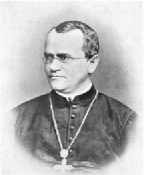
Gregor Mendel [1822–1884, Figure 1(a)] was an Augustinian Austrian monk who, during at least seven years, performed controlled crossing experiments with the garden pea (Pisum sativum L.). He may have personally controlled the fertilization of around 29,000 plants. Based on the results of these experiments, he formulated the two laws, or principles, of heredity (Mendel’s first law: principle of segregation; Mendel’s second law: principle of independent assortment). Mendel’s findings were published in 1866 in the Proceedings of the Society of Natural History of Brünn, Mendel (1866). To draw his conclusions, Mendel analyzed the data informally, that is, without using formal statistical methods, simply because the tools he needed did not exist. Yet he shows a remarkable intuition for statistical concepts, being quite aware of chance, variability and random errors. This shows how Mendel was a man far ahead of his time.

(a)	(b)

Figure 1: (a) Mendel’s portrait which appeared as frontispiece in the book Mendel’s Principles of Heredity, a Defense, Bateson (1902). (b) A picture of Sir R. A. Fisher.

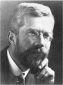
Sir Ronald Fisher [1890–1962, Figure 1(b)] made fundamental contributions to statistics and is also regarded as the founder of quantitative genetics. He is described by Hald (1998) as “a genius who almost single-handedly created the foundations for modern statistical science” and by Dawkins (1995) as “the greatest of Darwin’s successors.” It is thus quite understandable that Fisher became interested in Mendel’s work and data very early in his career.

Let us now review the chronology of this controversy:

1856–1863

Mendel performed his experiments during this period. He produced around 29,000 garden pea plants from controlled crosses and registered several of their observable characteristics (phenotype), such as shape and color of the seeds, height, flower color, etc.

1865

Mendel presented the results of his experiments in a communication entitled Experiments on Plant Hybridization, read at two meetings of the Society of Natural History of Brünn.

1866

The paper with the same title was published in the proceedings of that society. The paper had little impact and would be cited only three times in the next 35 years.

1900

His work was rediscovered independently by Hugo de Vries, Carl Correns and Erich von Tschermak.

1902

The first statistical analysis of Mendel’s data is published in the first volume of Biometrika (Weldon, 1902), using the then recently invented chi-square test (Pearson, 1900).

1911

Fisher produced a first comment about Mendel’s results, in a communication to the Cambridge University Eugenics Society, while he was still an undergraduate: “It is interesting that Mendel’s original results all fall within the limits of probable error” and suggested that Mendel may have “unconsciously placed doubtful plants on the side which favoured his hypothesis” (Franklin et al., 2008, page 16).

1936

Fisher published the paper Has Mendel’s work been rediscovered? (Fisher, 1936), where he expresses the same concern but this time presenting a detailed analysis, both of Mendel’s experiments and data. He also attributes the alleged forgery, not to Mendel himself, but to an unknown assistant: “Although no explanation can be expected to be satisfactory, it remains a possibility among others that Mendel was deceived by some assistant who knew too well what was expected” (Fisher, 1936, page 132). Fisher also questioned some other aspects of Mendel’s experiments, but those do not involve statistical aspects and will not be discussed here.

1964

The publication De Beer (1964), intended to celebrate the centennial of Mendel’s article, highlights the fact that Fisher “was able to reconstruct the sequence thread and development of Mendel’s series of experiments” and draws attention to Fisher’s work on the statistical analysis of Mendel’s results. Ironically, Fisher’s paper appears to have remained mostly overlooked until approximately this anniversary, as far as we can tell based on the scarcity of previous citations.

1964–2007

During this period at least 50 papers have been published about the controversy created by Fisher. Some elucidative titles: The too-good-to-be-true paradox and Gregor Mendel (Pilgrim, 1984); Are Mendel’s results really too close? (Edwards, 1986a); Mud Sticks: On the Alleged Falsification of Mendel’s Data (Hartl and Fairbanks, 2007).

2008

A group of scientists from different fields,Franklin (Physics and History of Science), Edwards (Biometry and Statistics, and curiously, Fisher’s last student), Fairbanks (Plant and Wildlife Sciences), Hartl (Biology and Genetics) and Seidenfeld (Philosophy and Statistics), who have previously published work on the controversy, merged their most relevant papers and published the book Ending the Mendel–Fisher Controversy. But is it really the end of the controversy? The authors dismiss all of the issues raised by Fisher except the “too good to be true” (pages 68 and 310).

In a very interesting book review, entitled CSI: Mendel, Stigler (2008) adds: “…an actual end to that discussion is unlikely to be a consequence of this book.” and “…thanks to these lucid, insightful and balanced articles, another generation will be able to join the quest with even better understanding.”

3 Experiments and Data

Before introducing the data and discussing the corresponding statistical analysis, it is important to understand the experiments and the scientific hypotheses under evaluation. Using a classification similar to that used by Fisher, the experiments can be classified as follows: single trait, bifactorial, trifactorial and gametic ratios experiments.

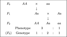
Single trait experiments. These concern the transmission of only one binary characteristic (or trait) at a time. Mendel examined seven traits, two observable in the seeds (seed shape: round or wrinkled; seed color: yellow or green) and five in the plants (flower color: purple or white; pod shape: inflated or constricted; pod color: yellow or green; flower position: axial or terminal; stem length: long or short). First Mendel obtained what are now called “pure lines,” with each of the two forms of the seven characters, that is, plants which yielded perfectly constant and similar offspring. When crossing the two pure lines, $F_{0}$, for each character Mendel observed that all the progeny, $F_{1}$, presented only one of the forms of the trait. He called this one the dominant form and represented it by $A$. The other form was called recessive and denoted by $a$. In the seven traits listed above the first form is the dominant and the second is the recessive. He then crossed the $F_{1}$ individuals (which he called the hybrids) and observed that in the resulting generation, $F_{2}$, there were individuals of the two original types, approximately in the ratio $3:1$ of the dominant type to the recessive type. In modern notation and terminology, we are studying a phenotype with possible values “$A$” and “$a$” governed by a single gene with two alleles ($A$ and $a$, where the first is dominant). The $F_{0}$ plants are homozygous $AA$ (genotype $AA$, phenotype “$A$”) or $aa$ (genotype $aa$, phenotype “$a$”), the $F_{1}$ are all heterozygous $Aa$ (genotype $Aa$, phenotype “$A$”), the $F_{2}$ plants can have genotype $AA$ (phenotype “$A$”), genotype $Aa$ (phenotype “$A$”) and genotype $aa$ (phenotype “$a$”). When Mendel self-fertilized the $F_{2}$ plants with phenotype “$A,$” he found that about one-third of these always produced phenotype “$A$” progeny, while about two-thirds produced phenotype “$A$” and phenotype “$a$” progeny in the ratio $3:1$. This process is schematically represented in Figure 2, where ($F_{3}$) refers to the progeny of the self-fertilized $F_{2}$ individuals.

Figure 2: A schematic representation of Mendel’s single trait experiments (in modern notation and terminology).

Table 1: Data given in Mendel (1866) for the single trait experiments. “$A$” (“$a$”) denotes the dominant (recessive) phenotype; $A$ ($a$) denotes the dominant (recessive) allele; $n$ is the total number of observations per experiment (that is, seeds for the seed trait experiments and plants otherwise); $n_{{{\textnormal{``{A}''}}}}$, $n_{{{\textnormal{``{a}''}}}}$, $n_{Aa}$ and $n_{AA}$ denote observed frequencies

					Obs. freq.		Theor. ratio
	Trait	“A”	“a”	$\bolds n$	$\bolds n_{{{\textbf{``{A}''}}}}$	$\bolds n_{{{\textbf{``{a}''}}}}$	$\mbox{{``{A}''}}\bolds:\mbox{{``{a}''}}$
	Seed shape	round	wrinkled	$7324$	$5474$	$1850$	$3:1$
	Seed color	yellow	green	$8023$	$6022$	$2001$	$3:1$
	Flower color	purple	white	$929$	$705$	$224$	$3:1$
$F_{2}$	Pod shape	inflated	constricted	$1181$	$882$	$299$	$3:1$
	Pod color	yellow	green	$580$	$428$	$152$	$3:1$
	Flower position	axial	terminal	$858$	$651$	$207$	$3:1$
	Stem length	long	short	$1064$	$787$	$277$	$3:1$
	Trait	$\bolds A$	$\bolds a$	$\bolds n$	$\bolds{n_{Aa}}$	$\bolds{n_{AA}}$	$\bolds{Aa:AA}$
	Seed shape	round	wrinkled	$565$	$372$	$193$	$2:1$
	Seed color	yellow	green	$519$	$353$	$166$	$2:1$
	Flower color	purple	white	$100$	$64$	$36$	$2:1$
$(F_{3})$	Pod shape	inflated	constricted	$100$	$71$	$29$	$2:1$
	Pod color	yellow	green	$100$	$60$	$40$	$2:1$
	Flower position	axial	terminal	$100$	$67$	$33$	$2:1$
	Stem length	long	short	$100$	$72$	$28$	$2:1$
	Pod color (rep.)	yellow	green	$100$	$65$	$35$	$2:1$

Table 1 presents the data given in Mendel (1866) for the single trait experiments just described. As an illustration of the variability of the results between plants, Mendel also presented the individual figures obtained for the ten first plants of each of the experiments relative to the seed characteristics (these are referred to by Fisher as “illustrations of plant variation,” cf. Table 5).

Table 2: Data from the bifactorial experiment [as organized by Fisher (1936)]

	$\bolds{AA}$	$\bolds{Aa}$	$\bolds{aa}$	Total
$BB$	138	160	128	126
$Bb$	165	138	168	271
$bb$	135	167	130	132
Total	138	265	126	529

Bifactorial experiment. This is an experiment similar to the single trait experiments but observing two characteristics simultaneously (seed shape, A, and seed color, B, starting from pure lines on both). The aim was to observe how the two traits are combined. Mendel postulated and confirmed from the results of the experiment that the traits considered are assorted independently. That is, given a trait A with an $F_{2}$ generation $AA$, $Aa$ and $aa$ in the ratio $1:2:1$, and a trait B with $BB$, $Bb$ and $bb$ in the same ratio, combining the two independently leads to the genotypes and theoretical ratios represented in Figure 3. The data, organized by Fisher from Mendel’s description, are shown in Table 2.

Table 3: Data from the trifactorial experiment [as organized by Fisher (1936)]

	$\bolds{CC}$				$\bolds{Cc}$				$\bolds{cc}$				Total
2-5,6-9,10-13,14-17	$\bolds{AA}$	$\bolds{Aa}$	$\bolds{aa}$	Total	$\bolds{AA}$	$\bolds{Aa}$	$\bolds{aa}$	Total	$\bolds{AA}$	$\bolds{Aa}$	$\bolds{aa}$	Total	$\bolds{AA}$	$\bolds{Aa}$	$\bolds{aa}$	Total
$BB$	18	14	18	130	22	138	25	185	14	18	10	142	144	170	143	157
$Bb$	15	49	19	183	45	178	36	159	18	48	24	190	178	175	179	332
$bb$	19	20	10	139	17	140	20	177	11	16	47	134	137	176	137	150
Total	32	83	37	152	84	156	81	321	43	82	41	166	159	321	159	639

Figure 3: Genotypes and theoretical ratios for the bifactorial experiment.

Figure 4: Theoretical ratios for the trifactorial experiment.

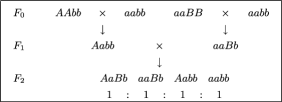
Trifactorial experiment. This experiment is also similar to the previous experiment but considering the crossing of three traits (seed shape, seed color and flower color). The data, organized by Fisher from Mendel’s description, are shown in Table 3, whereas the corresponding theoretical ratios are given in Figure 4.

Gametic ratios experiments. In this last series of experiments Mendel designed more elaborated crosses in order to obtain “conclusions as regards the composition of the egg and pollen cells of hybrids.” The crosses are represented in Figure 5 and the data are shown in Table 4.

We will also use an organization of the data into 84 binomial experiments, similar to the one proposed by Edwards (1986a, see also Franklin et al., 2008, Chapter 4). The data set used is described in detail in Appendix A.

All the computations and Monte Carlo simulations described were carried out using the R software (R Development Core Team, 2008). The full code is available upon request.

4 Statistical Analysis: Incriminating Evidence

4.1 Fisher’s Analysis

As mentioned in Section 2, Fisher (1936) presents a very detailed analysis of both Mendel’s experiments and data. Here we will concentrate on a particular part of the analysis, the chi-square analysis summarized in Table V, page 131, of Fisher (1936), which is reproduced in Table 5. This table has been the subject of a lot of debate, and it constitutes the main evidence for the “too good to be true” aspect of Mendel’s data as claimed by Fisher. We later present a new explanation for this evidence.

(a)

(b)

Figure 5: Schematic representation of the gametic ratios experiments: (a) experiments 1–4 in Table 4; (b) experiment 5 in Table 4.

Table 4: Data from the gametic ratios experiments (Mendel,1866)

Exp.	$\bolds n$	Observed frequencies				Theoretical ratio	Traits
							$\bolds A$	$\bolds B$
1	190	20	23	25	22	$1:1:1:1$	seed shape	seed color
2	110	31	26	27	26	$1:1:1:1$	seed shape	seed color
3	187	25	19	22	21	$1:1:1:1$	seed shape	seed color
4	198	24	25	22	27	$1:1:1:1$	seed shape	seed color
5	166	47	40	38	41	$1:1:1:1$	flower color	stem length

The analysis is very simple to describe: for each separate experiment, Fisher performed a chi-square goodness-of-fit test, where $H_{0}$ specifies the probabilities implied by the theoretical ratios. Note that, for the two category cases, this is equivalent to the usual asymptotic test for a single proportion. Then he aggregated all the tests by summing the chi-square statistics as well as the associated number of degrees of freedom and computed an aggregated $p$-value of 0.99993. This would mean that if Mendel’s experiments were repeated, under ideal conditions such that all the null-hypotheses are true, and all the Bernoulli trials—within and between experiments—are independent, the probability of getting an overall better result would be 7$/$100,000.

Fisher’s chi-square results were recomputed just to confirm that we are working with exactly the same data and assumptions. The results, given in the first 4 columns of Table 6, show that the statistics ($\chi^{2}_{\mathrm{obs}}$) are identical to Fisher’s values, but there are some differences in the $p$-values which certainly reflect different methods of computing the chi-square distribution function [$p$-value ($\chi^{2}_{\mathrm{df}}$) denotes the $p$-value computed from a $\chi^{2}$ distribution with $\mathit{df}$ degrees of freedom, that is, $P(\chi^{2}_{\mathrm{df}}>\chi^{2}_{\mathrm{obs}})$].

Table 5: Fisher’s chi-square analysis (“Deviations expected and observed in all experiments”)

Experiments	Expectation	$\bolds{\chi^{2}}$	Probability
			of exceeding
			deviations
			observed
$3:1$ ratios	$7$	$2.1389$	$0.95$
$2:1$ ratios	$8$	$5.1733$	$0.74$
Bifactorial	$8$	$2.8110$	$0.94$
Gametic ratios	$15$	$3.6730$	$0.9987$
Trifactorial	$26$	$15.3224$	$0.95$
Total	$64$	$29.1186$	$0.99987$
Illustrations of
plant variation	$20$	$12.4870$	$0.90$
Total	$84$	$41.6056$	$0.99993$

The table also gives the Monte Carlo (MC) estimates of the $p$-values (and corresponding standard errors, se) based on 1,000,000 random repetitions of the experiments using binomial or multinomial sampling, whichever is appropriate, as considered by Fisher. A more detailed description of the Monte Carlo simulation is given in Appendix B.1.

Comparing the list of $\chi^{2}_{\mathrm{df}}$ $p$-values with the list of MC $p$-values, the conclusion is that the approximation of the sampling distribution of the test statistic by the chi-square distribution is very accurate, and that Fisher’s analysis is very solid [our results are also in accordance with the results of similar but less extensive simulations described in Novitski (1995)]. Moreover, we can also conclude that the evidence “against” Mendel is greater than that given by Fisher, since an estimate of the probability of getting an overall better result is now 2$/$100,000. We have also repeated the chi-square analysis considering the 84 binomial experiments (results given in the next 3 columns of Table 6) and concluded that the two sampling models are almost equivalent, the second one (only binomial) being slightly more favorable to Fisher and less favorable to Mendel. Acting in Mendel’s defense, the results will be more convincing if we prove our case under the least favorable scenario. Thus, for the remaining investigation, we use only the binomial model and data set.

= Fisher (binomial $\bolds+$ multinomial) Model A Model B 9-11,12-14 Edwards (binomial) $\bolds{\alpha=0.094}$ $\bolds{\alpha=0.201}$ $\bolds{\alpha=0.362}$ $\bolds{\beta=0.261}$ $\bolds{\beta=0.455}$ $\bolds{\beta=0.634}$ 3-5,6-8,9-11,12-14 $\bolds p$-value $\bolds p$-value $\bolds p$-value $\bolds p$-value $\bolds p$-value $\bolds p$-value $\bolds p$-value $\bolds p$-value $\bolds p$-value $\bolds p$-value Exp. $\bolds{df}$ $\bolds{\chi^{2}_{\mathbf{obs}}}$ ($\bolds{\chi^{2}_{\mathbf{df}}}$) (MC) $\bolds{\chi^{2}_{\mathbf{obs}}}$ ($\bolds{\chi^{2}_{\mathbf{df}}}$) (MC) (MC) (MC) (MC) (MC) (MC) (MC) (se) (se) (se) (se) (se) (se) (se) (se) 3:1 67 $2.1389$ $0.9518$ $0.9519$ $2.1389$ $0.9518$ $0.9517$ $0.9069$ $0.8286$ $0.6579$ $0.9023$ $0.8446$ $0.7701$ $(0.0002)$ $(0.0002)$ $(0.0003)$ $(0.0004)$ $(0.0005)$ $(0.0003)$ $(0.0004)$ $(0.0004)$ 2:1 68 $5.1733$ $0.7389$ $0.7401$ $5.1733$ $0.7389$ $0.7393$ $0.4955$ $0.2374$ $0.1156$ $0.6044$ $0.4826$ $0.3586$ $(0.0004)$ $(0.0004)$ $(0.0005)$ $(0.0004)$ $(0.0003)$ $(0.0005)$ $(0.0005)$ $(0.0005)$ BF 68 $2.8110$ $0.9457$ $0.9462$ $2.7778$ $0.9475$ $0.9482$ $0.8838$ $0.7839$ $0.5926$ $0.8914$ $0.8248$ $0.7376$ $(0.0002)$ $(0.0002)$ $(0.0003)$ $(0.0004)$ $(0.0005)$ $(0.0003)$ $(0.0004)$ $(0.0004)$ GR 15 $3.6730$ $0.9986$ $0.9987$ $3.6277$ $0.9987$ $0.9987$ $0.9950$ $0.9811$ $0.9063$ $0.9939$ $0.9827$ $0.9584$ $(0.00004)$ $(0.00004)$ $(0.00007)$ $(0.0001)$ $(0.0003)$ $(0.00008)$ $(0.0001)$ $(0.0002)$ TF 26 $15.3224$ $0.9511$ $0.9512$ $15.1329$ $0.9549$ $0.9555$ $0.6973$ $0.2917$ $0.0812$ $0.8493$ $0.6941$ $0.4847$ $(0.0002)$ $(0.0002)$ $(0.0004)$ $(0.0005)$ $(0.0003)$ $(0.0004)$ $(0.0005)$ $(0.0005)$ Tot. 64 $29.1185$ $0.99995$ $0.99995$ $28.8506$ $0.99995$ $0.99995$ $0.9917$ $0.8175$ $0.2965$ $0.9980$ $0.9800$ $0.8887$ $(0.000007)$ $(0.000007)$ $(0.00008)$ $(0.0004)$ $(0.0005)$ $(0.00004)$ $(0.0001)$ $(0.0003)$ PV 20 $12.4870$ $0.8983$ $0.9000$ $12.4870$ $0.8983$ $0.9003$ $0.5932$ $0.2196$ $0.0684$ $0.7582$ $0.5922$ $0.4028$ $(0.0003)$ $(0.0003)$ $(0.0005)$ $(0.0004)$ $(0.0003)$ $(0.0004)$ $(0.0005)$ $(0.0005)$ Tot. 84 $41.6055$ $0.99997$ $0.99998$ $41.3376$ $0.99998$ $0.99998$ $0.9860$ $0.6577$ $0.1176$ $0.9980$ $0.9733$ $0.8348$ $(0.000005)$ $(0.000005)$ $(0.0001)$ $(0.0005)$ $(0.0003)$ $(0.00004)$ $(0.0002)$ $(0.0004)$

Table 6: Results of the chi-square analysis considering different models and methods for computing/estimating $p$-values. Each line corresponds to a different type of experiment in Mendel’s paper: single trait, $3:1$ ratios; single trait, $2:1$ ratios; bifactorial (BF); gametic ratios (GR); trifactorial (TF); and illustrations of plant variation (PV). $\mathit{df}$: degrees of freedom of the asymptotic distribution of the $\chi^{2}$ test statistic under $H_{0}$ (Mendel’s theory); $\chi^{2}_{\mathrm{obs}}$: observed value of the $\chi^{2}$ test statistic; $p$-value ($\chi^{2}_{\mathrm{df}}$): $p$-value computed assuming that the test statistic follows, under $H_{0}$, a $\chi^{2}$ distribution with $\mathit{df}$ degrees of freedom; $p$-value (MC): $p$-value estimated from Monte Carlo simulation. se: standard error of the $p$-value (MC) estimate

Franklin et al. (2008, pages 29–67) provide a comprehensive systematic review of all the papers published since the 1960s in reaction to Fisher’s accusations. The vast majority of those authors try to put forward arguments in Mendel’s defense. We only highlight here some of the more relevant contributions regarding specifically the “too good to be true” conclusion obtained from the chi-square analysis. The majority of the reactions/arguments can be generically classified into three categories.

In the first category we consider those who do not believe in Fisher’s analysis. This is the case of Pilgrim (1984, 1986) who in the first paper affirms to have detected “four paradoxical elements in Fisher’s reasoning” and who, in the second, claims to have been able to show where Fisher went wrong. Pilgrim’s arguments are related to the application of the chi-square global statistic and were refuted by Edwards (1986b).

As a second category, those who, in spite of believing that Fisher’s analysis is correct, think it is too demanding and propose alternative ways to analyze Mendel’s data. Edwards (1986a) analyzes the distribution of a set of test statistics, whereas Seidenfeld (1998) analyzes the distribution of a set of $p$-values. They both find the “too good to be true” characteristic and come to the conclusion that Mendel’s results were adjusted rather than censored. The methods of Leonard (1977) and Robertson (1978), who analyzed only a small part of the data, could also be classified here, but, according to Piegorsch (1983), their contribution to advance the debate was marginal.

Finally, as a third category, those who believeFisher’s analysis is correct under its assumptions (binomial/multinomial sampling, independent experiments) and then try to find a reason or explanation, other than deliberate cheating, for the observation of a very high global $p$-value. Such an explanation has to imply the failure of at least one of those two assumptions. Moreover, that failure has to occur in a specific direction, the one which would reduce the chi-square statistics: for instance, the distribution of the phenotypes is not binomial and has a smaller variance than the binomial. The various explanations that have been put forward can be divided into the following: biological, statistical and methodological.

Among the biological candidate explanations, one that received some attention was the “Tetrad Pollen Model” (see Fairbanks and Schaalje, 2007).

Few purely statistical explanations have been proposed and most of them are anecdotal. One that raised some discussions was a proposal of Weiling (1986) who considers, based on the tetrad pollen model just mentioned, a distribution with smaller variance than the binomial for some of the experiments, and hypergeometric for other experiments.

The majority of the suggested explanations are of a methodological nature: the “anonymous” assistant (Fisher); sequential procedures, like stopping the count when the results look good (several authors); discard plants or complete experiments due to suspicions of some experimental error, like pollen contamination (Dobzhansky, 1967); luck(?); inherent difficulties in the classification of the phenotypes (Root-Bernstein, 1983); data selection for presentation (Di Trocchio, 1991; Fairbanks and Rytting, 2001).

It is important to keep in mind that for an explanation to be acceptable as the solution to the controversy it must fulfill a number of conditions: (i) it must be biologically plausible and/or experimentally verifiable; (ii) it must be statistically correct and pass the chi-square and eventually other statistical analyses aiming at disentangling the enigma; and (iii) assuming that Mendel’s theory is correct and that he is not guilty of any deliberate fraud, it has to find support in and it can not contradict Mendel’s writings. The fact is that all the explanations which were proposed up to now failed in one or other of these requirements.

In summary, Fisher’s analysis has resisted all attempts to be either refuted or explained. Our simulation also confirms that, under the standard assumptions, Fisher’s tests and conclusions are correct.

4.2 Analysis of $p$-Values

As mentioned in Section 3, Edwards (1986a) proposed an organization of the data into 84 binomial experiments. He then used the data to compute what he called (signed) $\chi$ values, that is, the square root of the chi-square statistic with the sign of the deviation (“$+$” if observed $>$ expected and “$-$” if observed $<$ expected). Since all the tests have one degree of freedom and, assuming that Mendel’s theory is correct, the $\chi$ values should follow approximately a standard normal distribution. However, a normal qqplot of those values shows apparently a large deviation from normality (Franklin et al., 2008, Figures 1.1 and 1.2, page 49). From the shape of the plot Edwards (1986a) concluded that it appears to be more likely that Mendel’s results were adjusted rather than truncated. This conclusion, to which Seidenfeld (1998) also arrives, and later Franklin et al. (2008) agree, would render some of the most plausible methodological explanations not viable.

Another approach is to analyze the $p$-values of the individual $\chi^{2}_{1}$ tests. This idea was explored by Seidenfeld (1998); (see also Franklin et al., 2008, Figures 1.3 and 1.4, page 59), although not so systematically as in the analysis provided here. The 84 $\chi$ values, along with the 84 $p$-values, are also given in Appendix A.

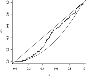
As for Fisher’s and Edwards’ analysis, we know what to expect under the ideal assumptions. That is, if: (i) Mendel’s theory is valid for all the experiments, or, equivalently, if the null hypotheses of the chi-square tests are true in all cases; (ii) the experiments were performed independently and as described in Mendel’s paper; and (iii) the chi-square approximation is valid, then the $p$-values follow a uniform $(0,1)$ distribution. Therefore, the plot of the empirical cumulative distribution function (e.c.d.f.) of the $p$-values should be close to the diagonal of the $(0,1)\times(0,1)$ square. However, the e.c.d.f., plotted in Figure 6, reveals a marked difference from uniformity. This visual assertion was confirmed by a Kolmogorov–Smirnov (K–S) goodness-of-fit test ($p$-value${}=0.0036$, details in Appendix B.2). We can therefore conclude with a high confidence that the distribution of the $p$-values deviates from a uniform $(0,1)$ distribution. It is then natural to wonder about the kind of deviation and its meaning. In Figure 6 we also plot the cumulative distribution function (c.d.f.) of the maximum of two uniform $(0,1)$ random variables, $y=x^{2}$, since this is central to the explanation that we give later for Mendel’s results.

Figure 6: Empirical cumulative distribution function of the $p$-values (stair steps line); cumulative distribution function of the uniform $(0,1)$ random variable (straight line); cumulative distribution function of the maximum of two $(0,1)$ uniform random variables (curve).

Figure 7: Histogram of the 84 $p$-values observed [the dashed line indicates the expected frequencies under the uniform $(0,1)$ distribution].

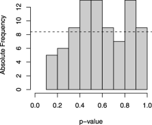
The histogram of the $p$-values (Figure 7) is helpful for our argumentation. One could perhaps think that the uniform distribution is not a good fit for the sample of $p$-values because some of the null hypotheses are not true. But if that were the case, we would observe an excess of values close to 0, and the histogram shows precisely the opposite. Possible reasons for this to happen are as follows: either the data shows that the hypotheses are “more true,” that is, the data are better than expected under the null hypotheses, or there is something wrong with the assumptions (and possible explanations are, as for the chi-square analysis, smaller variance than binomial, or lack of independence).

In conclusion, the $p$-value analysis shows that the probability of obtaining overall results as good or better than those obtained by Mendel (under the assumptions) is about 4$/$1000. This “evidence” is not as extreme as the 2$/$100,000 resulting from the chi-square analysis but points in the same direction.

5 A Plausible Explanation

5.1 A Statistical Model for the $p$-Values

In the previous section we have shown that there is strong evidence that the $p$-values are not uniformly distributed. What is then their distribution, and how can it be explained?

The shape of the e.c.d.f. provides a hint: it resembles the function $x^{2}$, which is the c.d.f. of the maximum of two uniform $(0,1)$ random variables, as can easily be shown. It appears that some c.d.f. intermediate between that corresponding to a uniform $(0,1)$ random variable and that corresponding to the maximum of two uniform $(0,1)$ random variables best fits the e.c.d.f. of the sample $p$-values (see Figure 6).

One explanation for this is the following: suppose Mendel has repeated some experiments, presumably those which deviate most from his theory, and reports only the best of the two. A related possibility was suggested by Fairbanks and Rytting (2001, page 743): “We believe that the most likely explanation of the bias in Mendel’s data is also the simplest. If Mendel selected for presentation a subset of his experiments that best represented his theories, $\chi^{2}$ analysis of those experiments should display a bias.” The authors support this explanation with citations from Mendel’s work. We have found only an attempt to verify the effect of such a selection procedure on the chi-square analysis (footnote number 62, page 73, of Franklin et al., 2008), but it seems to lead to the wrong conclusion, as we conclude later that the effect of the given explanation on the chi-square analysis is very small. Moreover, the explanation appears to have been abandoned because “It does not [however] address the demonstration, by both Edwards and Seidenfeld, that Mendel’s data had not merely been truncated, but adjusted” (Franklin et al., 2008, page 62).

Both procedures described in the previous paragraph for selecting the data to be presented can be modeled by assuming that an experiment is repeated whenever its $p$-value is smaller than $\alpha$, where $0\leq\alpha\leq 1$ is a parameter fixed by the experimenter, and then only the one with the largest $p$-value is reported. Under this selection model (from now on named “model A”), the c.d.f. of the $p$-values of the experiments reported is given by

$$\qquad F_{\alpha}(x)=\cases{\displaystyle x^{2},&if $0\leq x\leq\alpha$,\cr\displaystyle(1+\alpha)x-\alpha,&if $\alpha<x\leq 1$.}$$ (1)

For a given experiment, denote by $X$ the $p$-value effectively reported. We have that $X=X_{1}$, if $X_{1}\geq\alpha$ and $X=\max(X_{1},X_{2})$ if $X_{1}<\alpha$, where $X_{1}$ and $X_{2}$ represent the $p$-values obtained in the first and the second realization of the experiment (if there is one), respectively. Assume that $X_{1}$ and $X_{2}$ are independent and identically distributed continuous uniform $(0,1)$ random variables (i.e., the two realizations of the experiment are independent and the associated null hypothesis is true), that is, $P(X_{1}\leq x)=P(X_{2}\leq x)=x$, $0\leq x\leq 1$. In the derivation of $F_{\alpha}(x)=P(X\leq x)$, the cases $0\leq x<\alpha$ and $\alpha\leq x\leq 1$ are considered separately.

If $0\leq x<\alpha$,

$$P(X\leq x) = P\bigl{(}\max(X_{1},X_{2})\leq x\bigr{)}$$

$$= P(\{X_{1}\leq x\}\cap\{X_{2}\leq x\})$$

$$= P(X_{1}\leq x)P(X_{2}\leq x)=x^{2}.$$

If $\alpha\leq x\leq 1$,

$$P(X\leq x)$$

$$\quad=P\bigl{(}(\{X\leq x\}\cap\{X_{1}<\alpha\})$$

$$\qquad\hphantom{P}{}\cup(\{X\leq x\}\cap\{X_{1}\geq\alpha\})\bigr{)}$$

$$\quad=P(\{X\leq x\}\cap\{X_{1}<\alpha\})$$

$$\qquad{}+P(\{X\leq x\}\cap\{X_{1}\geq\alpha\})$$

$$\quad=P\bigl{(}\{\max(X_{1},X_{2})\leq x\}\cap\{X_{1}<\alpha\}\bigr{)}$$

$$\qquad{}+P(\{X_{1}\leq x\}\cap\{X_{1}\geq\alpha\})$$

$$\quad=P(\{X_{1}<\alpha\}\cap\{X_{2}\leq x\})+P(\alpha\leq X_{1}\leq x)$$

$$\quad=x\times\alpha+(x-\alpha).$$

Suppose that model A holds but $\alpha$ is unknown and must be estimated using the available sample of 84 binomial $p$-values. The minimum distance estimator based on the Kolmogorov distance, also called the “Minimum Kolmogorov–Smirnov test statistic estimator” (Easterling, 1976), provides one method for estimating $\alpha$. This estimate is the value of $\alpha$ which minimizes the K–S statistic,

$$D(\alpha)=\sup_{x}|F_{n}(x)-F_{\alpha}(x)|$$ (2)

for testing the null hypothesis that the c.d.f. of the $p$-values is $F_{\alpha}$. Equivalently, the estimate can be determined by finding the value of $\alpha$ which maximizes the $p$-value of the K–S test, $p(\alpha)$, since $p(\cdot)$ is a strictly decreasing function of $D(\cdot)$.

Figure 8: Plot of the $p$-value of the K–S test as a function of the parameter, showing the point estimate and the 90% confidence interval, for model A.

Figure 9: Empirical cumulative distribution function of the $p$-values and fitted model (solid line: $\hat{\alpha}=0.201$; dashed lines: 90% confidence limits).

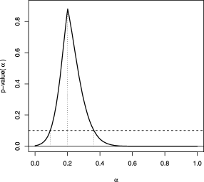
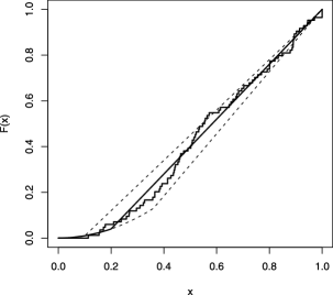
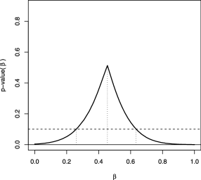
Figure 8 shows the plot of the K–S $p$-values, $p(\alpha)$, as a function of $\alpha$, together with the point estimate, $\hat{\alpha}=0.201$ ($D=0.0623$, $P=0.8804$), and a 90% confidence interval for $\alpha,(0.094;0.362)$. A detailed explanation on how these figures were obtained is given in Appendix B.3. Figure 9 confirms the good model fit.

This model can also be submitted to Fisher’s chi-square analysis. Assuming it holds for a certain value $\alpha_{0}$, we may still compute “chi-square statistics,” but the $p$-values can no longer be obtained from the chi-square distribution. However, they can be accurately estimated by Monte Carlo simulation. The difference to the previous simulations is that statistics and ($\chi^{2}_{1}$) $p$-values were always computed (for each of the 84 binomial cases and each random repetition) and whenever that $p$-value was smaller than $\alpha_{0}$ another binomial result was generated and the statistic recorded was the minimum of the two.

The simulation results obtained for three values of $\alpha$ (point estimate and limits of the confidence interval) are presented in the three columns of Table 6 under the heading “Model A.” The $p$-values in these columns (and especially those corresponding to $\alpha=0.201$) do not show any sign of being too close to one anymore, in fact, they are perfectly reasonable. In Appendix C we present a more detailed (and technical) justification of the results obtained.

Figure 10: Plot of the $p$-value of the K–S test as a function of the parameter, showing the point estimate and the 90% confidence interval, for model B.

The conclusion is that our model explains Fisher’s chi-square results: Mendel’s data are “too good to be true” according to the assumption that all the data presented in Mendel’s paper correspond to all the experiments Mendel performed, or to a random selection from all the experiments. When this assumption is replaced by model A the results can no longer be considered too good. So we conclude that model A is a reasonable statistical explanation for the controversy. We do not pretend that it is necessarily the “true” model; however, it is very simple and does provide extra insight into the complexity of this historical debate and in this sense it is useful. As G.E.P. Box said, “All models are wrong, some models are useful.”

We have just seen how the suggested selection mechanism can make Mendel’s results (which we know are in fact correct) look too correct. This raises a related question of general interest to all experimental sciences: is it possible to make an incorrect theory look correct by applying this or a similar selection mechanism? Although a detailed answer to this question is beyond the scope of this paper, in Appendix D we give an idea on how a generalization of model A can be used to explore the question.

5.2 Alternative Models

No doubt there are many models, perhaps more complicated than ours, that explain Mendel’s data as well as, or perhaps better than, ours. A relevant question to ask, then, is whether any model similar to ours, more specifically, a one parameter model with c.d.f. varying between $x$ and $x^{2}$, would produce similar results and also a reasonable interpretation.

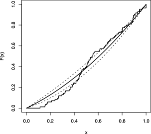
To show that the answer to this question is negative, we have considered an alternative model, model B, with distribution function computed as a linear combination of the “extreme” models, that is, with c.d.f. given by $F_{\beta}(x)=(1-\beta)\times x+\beta\times x^{2}$, with $0\leq\beta\leq 1$. This is mathematically simpler than model A and its interpretation in terms of the design of the experiments could be: Mendel would also decide to repeat some experiments and report only the best result of both (the original and the repetition), but the decision to repeat would be taken randomly with probability $\beta$, for instance, by throwing a fair coin ($\beta=0.5$) or something similar. Applying the methods described in Appendix B.3 to this model, we obtain (see Figure 10) $\hat{\beta}=0.45$ (K–S test: $D=0.0875$, $P=0.5131$) and $\mathit{CI}_{90\%}(\beta)=(0.261;0.634)$. Figure 11 shows the e.c.d.f. of the $p$-values and the c.d.f. of model B with $\beta=0.45$ (solid line) and $\beta=0.261,0.634$ (dashed lines). Compared to Figure 9, the fit of model B looks worse than the fit of model A, but it could still be considered acceptable. However, in what concerns the chi-square analysis, model B is unable to produce good results (cf. the last three columns in Table 6). The aggregated $p$-value (84 $\mathit{df}$) still points to “too good to be true” except maybe for the last column, which corresponds to the odd situation of randomly repeating about 60% of the experiments! We have presented model B as just an exercise to show a specific point, it does not correspond to a plausible procedure as does model A.

Figure 11: E.c.d.f. of the $p$-values and alternative model (solid line: $\hat{\beta}=0.45$; dashed lines: 90% confidence limits).

Figure 12: Each part of the figure contains a normal quantile–quantile plot of the original 84 Edwards’ $\chi$ values (solid thick line), and of 100 samples of simulated 84 $\chi$ values from each model (gray thin lines) as well as an intermediate line, located in the “middle” of the gray lines, corresponding to a “synthetic” sample obtained by averaging the ordered observations of the 100 simulated samples.

5.3 Further Support for the Proposed Model

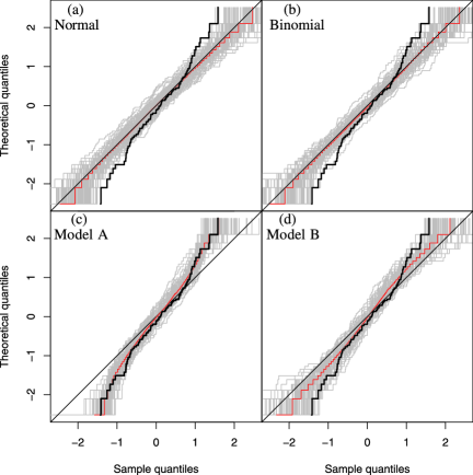
As a harder challenge, we observed the behavior of each of the models in the context of Edwards’ chi values analysis, mentioned at the beginning of Section 4.2. The results of a simple simulation exercise are represented in the four plots in Figure 12. All the plots are normal quantile–quantile plots, and contain the representation of the actual sample of 84 $\chi$ values (thick line). Each plot also represents 100 samples of simulated 84 $\chi$ values, generated by the corresponding model (gray thin lines), plus a “synthetic” sample obtained by averaging the ordered observations of those 100 simulated samples (intermediate line). Plot (a): the samples were generated from a standard normal random variable (i.e., from the asymptotic distribution of the $\chi$ values under the ideal assumptions, binomial sampling and independent experiments). Plot (b): in this case the $\chi$ values were obtained (by transformation of the $\chi^{2}$ values) from the first 100 samples used to obtain the results given in the columns with heading “Edwards” in Table 6. Plot (c): similar to the previous but with the samples generated under model A. Plot (d): idem with model B.

From the top plots we conclude that the Normal and the Binomial models are very similar and do not explain the observed values, whereas from the bottom plots we can see that model A provides a much better explanation of the $\chi$ values observed than model B. These conclusions are no longer surprising, in the face of the previous evidence; however, we shall remark that the several analyses are not exactly equivalent, so the previous conclusions would not necessarily imply this last one.

Besides the statistical evidence, which by itself may look speculative, the proposed model is supported by Mendel’s own words. The following quotations from Mendel’s paper (Mendel, 1866, page numbers from Franklin et al., 2008) are all relevant to our interpretation:

“it appears to be necessary that all members of the series developed in each successive generation should be, without exception, subjected to observation” (page 80).

From this sentence we conclude that Mendel was aware of the potential bias due to incomplete observation, thus, it does not seem reasonable that he would have deliberately censored the data or used sequential sampling as suggested by some authors:

“As extremes in the distribution of the two seed characters in one plant, there were observed in Expt. 1 an instance of 43 round and only 2 angular, and another of 14 round and 15 angular seeds. In Expt. 2 there was a case of 32 yellow and only 1 green seed, but also one of 20 yellow and 19 green” (page 86).

“Experiment 5, which shows the greatest departure, was repeated, and then in lieu of the ratio of 60 : 40, that of 65 : 35 resulted” (page 89).

Here he mentions repetition of an experiment but gives both results (note that he decided to repeat an experiment with $p$-value${}=0.157$). However, later he mentions several further experiments (pages 94, 95, 99, 100, 113) but presents results in only one case (page 99) and in another suggests that the results were not good (page 95):

“In addition, further experiments were made with a smaller number of experimental plants in which the remaining characters by twos and threes were united as hybrids: all yielded approximately the same results” (page 94).

“An experiment with peduncles of different lengths gave on the whole a fairly satisfactory results, although the differentiation and serial arrangement of the forms could not be effected with that certainty which is indispensable for correct experiment” (page 95).

“In a further experiment the characters of flower-color and length of stem were experimented upon…” in this case results are given, and then concludes “The theory adduced is therefore satisfactorily confirmed in this experiment also” (pages 99/100).

“For the characters of form of pod, color of pod, and position of flowers, experiments were also made on a small scale and results obtained in perfect agreement” (page 100).

“Experiments which in this connection were carried out with two species of Pisum …  The two experimental plants differed in 5 characters, …” (page 113).

It is likely that the results omitted were worse and that Mendel may have thought there would be no point in showing them anymore (he gave examples of bad fit to his theory before, page 86).

Our model may be seen as an approximation for the omissions described by Mendel. In conclusion, an unconscious bias may have been behind the whole process of experimentation and if that is accepted, then it explains the paradox and ends the controversy at last.

6 Conclusion

Gregor Mendel is considered by many a creative genius and incontestably the founder of genetics. However, as with many revolutionary ideas, his laws of heredity (Mendel, 1866), a brilliant and impressive achievement of the human mind, were not immediately recognized, and stayed dormant for about 35 years, until they were rediscovered in 1900. When Ronald Fisher, famous statistician and geneticist, considered the father of modern statistics, used a chi-square test to examine meticulously the data that Mendel had provided in his classical paper to prove his theory, he concluded that the data was too close to what Mendel was expecting, suggesting that scientific misconduct had been present in one way or another. This profound conflict raised a longstanding controversy that has been engaging the scientific community for almost a century. Since none of the proposed explanations of the conflict is satisfactory, a large number of arguments, ideas and opinions of various nature (biological, psychological, philosophical, historical, statistical and others) have been continually put forward just like a never ending saga.

This study relies on the particular assumption that the experimentation leading to the data analyzed by Fisher was carried out under a specific unconscious bias. The argument of unconscious bias has been considered a conceivable justification by various authors who have committed themselves to study some variations of this line of reasoning (Root-Bernstein, 1983; Bowler, 1989; Dobzhansky, 1967; Olby, 1984; Meijer, 1983; Rosenthal, 1976; Thagard, 1988; Nissani and Hoefler-Nissani, 1992). But all these attempts are based on somehow subjective interpretations and throw no definite light on the problem. On the contrary, in this paper the type of unconscious bias is clearly identified and a well-defined statistical analysis based on a proper statistical model is performed. The results show that the model is a plausible statistical explanation for the controversy.

The study goes as follows: (i) Fisher results were confirmed by repeating his analysis on the same real set of data and on simulated data, (ii) inspired by Edwards’ (1986a) approach, we next idealized a convenient model of a sequence of binomial experiments and recognized that the $p$-value produced by this model shows a slight increase, although it keeps very close to the result obtained by Fisher. This gave us confidence to work with this advantageous structure, (iii) we focused on the analysis of the $p$-values of the previous model and realized that the $p$-values do not have a uniform distribution as they should, (iv) the question arose of what the distribution of the $p$-values could be, and we arrived at the satisfactory model we propose in the text, (v) finally, assuming that our model holds, and repeating the chi-square analysis adopted by Fisher, one sees that the impressive effect detected by Fisher disappears.

Returning to Fisher’s reaction to the paradoxical situation he encountered, one may think that, despite his remarkable investigation (Fisher, 1936) of Mendel’s work, to prove that something had gone wrong with the selection of the experimental data, apparently neither did he question how could the data have been generated nor did he identify the defects of the sample or give a statistical explanation for the awkward result. In the end Fisher left an inescapable global impression of scientific malpractice, a conclusion that he based on a sound statistical analysis.

Probity is an essential component of the scientific work that should always be contemplated to guarantee credible final results and conclusions. That is why all measures should be taken to make sure that neither conscious nor unconscious bias will affect the results of the research work. Unfortunately there exists unconscious bias, an intrinsic automatic human drive based on culture, social prejudice or motivation that is difficult to stop. Hidden bias influences many aspects of our decisions, our social behaviour and our work. That is why scientific enterprises including honourable doctors and well-intentioned patients do not dispense the scientific techniques based on blind or double blind procedures. In Mendel’s case we all know that there was a profound motivation that could have triggered the bias and in those days we guess that the attention given to unconscious bias may have been poor or it may have not existed at all. Frequently science ends up in detecting errors or fraud that have been induced by bias. But there are no errors in Mendel’s laws, or are there? So why are we worried? Anyway, we wish that Mendel’s unconscious bias coincides with the arrangement we are suggesting in this paper, because if Mendel did what we think he did, the controversy is finally over.

Appendix A The 84 Binomial Experiments

Edwards (1986a) organized Mendel’s data as the result of 84 binomial experiments. Note that this involves decomposition of the multinomial experiments. In this study we have relied on Edwards’ decompositions. In order to remain as close as possible to Fisher’s choices, the data from Table 1—already binomial experiments—were included exactly asshown, unlike Edwards who subtracted the “plant illustrations” from these data. According to this procedure, experiment No. 1 (No. 2) is not independent of the “plant illustrations” Nos 8–17 (Nos 18–27). But, attending to the relative magnitude of the number of observations, if we had used Edwards’ numbers, the final results would have not been too different and the conclusions would have been the same. We have also considered the theoretical ratio of $2:1$ throughout the experiments involving $(F_{3})$ generations, instead of the ratio $0.63:0.37$ that Edwards used in some cases. The number of binomial experiments per pair of true probabilities (ratio) is as follows: 42 cases with $0.75:0.25$ ($3:1$); 15 cases with $0.5:0.5$ ($1:1$); 27 cases with $2/3:1/3$ ($2:1$).

Table 7 contains the following information about the 84 binomial experiments considered in this paper:

Trait:

binary variable under consideration (the category of interest is called a “success” and the other category is a “failure”) using the following coding: A (seed shape, round or wrinkled), B (seed color, yellow or green), C (flower color, purple or white), D (pod shape, inflated or constricted), E (pod color, yellow or green), F (flower position, axial or terminal), G (stem length, long or short). The usual notation is used to distinguish phenotype (italic inside quotation marks) from genotype (italic), and the dominant form (upper case) from the recessive (lowercase); see also Section 3 and Table 1.

$\bolds{n}$:

number of observations (Bernoulli trials) of the experiment.

Observed:

observed frequencies of “successes” ($n_{1}$) and “failures” ($n-n_{1}$). Under the standard assumptions $n_{1}\sim\operatorname{Bin}(n,p)$, where $p$ is the probability of a “success” in one trial.

$\bolds{p_{0}}$:

theoretical probability of a “success” underMendel’s theory ($H_{0}\dvtx p=p_{0}$).

$\bolds{\chi}$:

observed value of the test statistic to test $H_{0}$ against $H_{1}\dvtx p\neq p_{0}$, given by $(n_{1}-np_{0})/\break\sqrt{np_{0}(1-p_{0})}$.

$\bolds p$-value:

$p$-value of the test. Assuming $n$ is large, $p$-value${}=P(\chi_{1}^{2}>\chi^{2})$.

Table 7: Data from the 84 binomial experiments

Type of experiment				Observed
	No.	Trait	$\bolds n$	$\bolds{n_{1}}$	$\bolds{n-n_{1}}$	$\bolds{p_{0}}$	$\bolds\chi$	$\bolds p$-value
Single trait	$1$	A	$7324$	$5474$	$1850$	3$/$4	$-0.513$	0.608
$F_{2}$	$2$	B	$8023$	$6022$	$2001$	3$/$4	$0.123$	0.903
	$3$	C	$929$	$705$	$224$	3$/$4	$0.625$	0.532
	$4$	D	$1181$	$882$	$299$	3$/$4	$-0.252$	0.801
	$5$	E	$580$	$428$	$152$	3$/$4	$-0.671$	0.502
	$6$	F	$858$	$651$	$207$	3$/$4	$0.591$	0.554
	$7$	G	$1064$	$787$	$277$	3$/$4	$-0.779$	0.436
Illustrations	$8$	A	$57$	$45$	$12$	3$/$4	$0.688$	0.491
of plant	$9$	A	$35$	$27$	$8$	3$/$4	$0.293$	0.770
variation	$10$	A	$31$	$24$	$7$	3$/$4	$0.311$	0.756
$F_{2}$	$11$	A	$29$	$19$	$10$	3$/$4	$-1.179$	0.238
	$12$	A	$43$	$32$	$11$	3$/$4	$-0.088$	0.930
	$13$	A	$32$	$26$	$6$	3$/$4	$0.817$	0.414
	$14$	A	$112$	$88$	$24$	3$/$4	$0.873$	0.383
	$15$	A	$32$	$22$	$10$	3$/$4	$-0.817$	0.414
	$16$	A	$34$	$28$	$6$	3$/$4	$0.990$	0.322
	$17$	A	$32$	$25$	$7$	3$/$4	$0.408$	0.683
	$18$	B	$36$	$25$	$11$	3$/$4	$-0.770$	0.441
	$19$	B	$39$	$32$	$7$	3$/$4	$1.017$	0.309
	$20$	B	$19$	$14$	$5$	3$/$4	$-0.133$	0.895
	$21$	B	$97$	$70$	$27$	3$/$4	$-0.645$	0.519
	$22$	B	$37$	$24$	$13$	3$/$4	$-1.424$	0.155
	$23$	B	$26$	$20$	$6$	3$/$4	$0.227$	0.821
	$24$	B	$45$	$32$	$13$	3$/$4	$-0.603$	0.547
	$25$	B	$53$	$44$	$9$	3$/$4	$1.348$	0.178
	$26$	B	$64$	$50$	$14$	3$/$4	$0.577$	0.564
	$27$	B	$62$	$44$	$18$	3$/$4	$-0.733$	0.463
Bifactorial	$28$	A	$556$	$423$	$133$	3$/$4	$0.588$	0.557
experiment	$29$	B among “A”	$423$	$315$	$108$	3$/$4	$-0.253$	0.801
$F_{2}$	$30$	B among “a”	$133$	$101$	$32$	3$/$4	$0.250$	0.802
Trifactorial	$31$	A	$639$	$480$	$159$	3$/$4	$0.069$	0.945
experiment	$32$	B among “A”	$480$	$367$	$113$	3$/$4	$0.738$	0.461
$F_{2}$	$33$	B among “a”	$159$	$122$	$37$	3$/$4	$0.504$	0.615
	$34$	C among AaBb	$175$	$127$	$48$	3$/$4	$-0.742$	0.458
	$35$	C among AaBB	$70$	$52$	$18$	3$/$4	$-0.138$	0.890
	$36$	C among AABb	$78$	$60$	$18$	3$/$4	$0.392$	0.695
	$37$	C among AABB	$44$	$30$	$14$	3$/$4	$-1.045$	0.296
	$38$	C among Aabb	$76$	$60$	$16$	3$/$4	$0.795$	0.427
	$39$	C among AAbb	$37$	$26$	$11$	3$/$4	$-0.664$	0.506
	$40$	C among aaBb	$79$	$55$	$24$	3$/$4	$-1.104$	0.269
	$41$	C among aaBB	$43$	$33$	$10$	3$/$4	$0.264$	0.792
	$42$	C among aabb	$37$	$30$	$7$	3$/$4	$0.854$	0.393
Single trait	$43$	A	$565$	$372$	$193$	2$/$3	$-0.417$	0.677
($F_{3}$)	$44$	B	$519$	$353$	$166$	2$/$3	$0.652$	0.515
	$45$	C	$100$	$64$	$36$	2$/$3	$-0.566$	0.572
	$46$	D	$100$	$71$	$29$	2$/$3	$0.919$	0.358
	$47$	E	$100$	$60$	$40$	2$/$3	$-1.414$	0.157
	$48$	F	$100$	$67$	$33$	2$/$3	$0.071$	0.944
	$49$	G	$100$	$72$	$28$	2$/$3	$1.131$	0.258
	$50$	E	$100$	$65$	$35$	2$/$3	$-0.354$	0.724

Table 7: (Continued)

Type of experiment				Observed
	No.	Trait	$\bolds n$	$\bolds{n_{1}}$	$\bolds{n-n_{1}}$	$\bolds{p_{0}}$	$\bolds\chi$	$\bolds p$-value
Bifactorial	$51$	A among “AB”	$301$	$198$	$103$	2$/$3	$-0.326$	0.744
experiment	$52$	A among “Ab”	$102$	$67$	$35$	2$/$3	$-0.210$	0.834
($F_{3}$)	$53$	B among “aB”	$96$	$68$	$28$	2$/$3	$0.866$	0.386
	$54$	B among Aa“B”	$198$	$138$	$60$	2$/$3	$0.905$	0.366
	$55$	B among AA“B”	$103$	$65$	$38$	2$/$3	$-0.766$	0.443
Trifactorial	$56$	A among “AB”	$367$	$245$	$122$	2$/$3	$0.037$	0.971
experiment	$57$	A among “Ab”	$113$	$76$	$37$	2$/$3	$0.133$	0.894
($F_{3}$)	$58$	B among “aB”	$122$	$79$	$43$	2$/$3	$-0.448$	0.654
	$59$	B among Aa“B”	$245$	$175$	$70$	2$/$3	$1.581$	0.114
	$60$	B among AA“B”	$122$	$78$	$44$	2$/$3	$-0.640$	0.522
	$61$	C among AaBb	$127$	$78$	$49$	2$/$3	$-1.255$	0.210
	$62$	C among AaBB	$52$	$38$	$14$	2$/$3	$0.981$	0.327
	$63$	C among AABb	$60$	$45$	$15$	2$/$3	$1.369$	0.171
	$64$	C among AABB	$30$	$22$	$8$	2$/$3	$0.775$	0.439
	$65$	C among Aabb	$60$	$40$	$20$	2$/$3	$0.000$	1.000
	$66$	C among AAbb	$26$	$17$	$9$	2$/$3	$-0.139$	0.890
	$67$	C among aaBb	$55$	$36$	$19$	2$/$3	$-0.191$	0.849
	$68$	C among aaBB	$33$	$25$	$8$	2$/$3	$1.108$	0.268
	$69$	C among aabb	$30$	$20$	$10$	2$/$3	$0.000$	1.000
Gametic	$70$	A	$90$	$43$	$47$	1$/$2	$-0.422$	0.673
ratios	$71$	B among AA	$43$	$20$	$23$	1$/$2	$-0.458$	0.647
	$72$	B among Aa	$47$	$25$	$22$	1$/$2	$0.438$	0.662
	$73$	A	$110$	$57$	$53$	1$/$2	$0.381$	0.703
	$74$	B among Aa	$57$	$31$	$26$	1$/$2	$0.662$	0.508
	$75$	B among aa	$53$	$27$	$26$	1$/$2	$0.137$	0.891
	$76$	A	$87$	$44$	$43$	1$/$2	$0.107$	0.915
	$77$	B among AA	$44$	$25$	$19$	1$/$2	$0.905$	0.366
	$78$	B among Aa	$43$	$22$	$21$	1$/$2	$0.153$	0.879
	$79$	A	$98$	$49$	$49$	1$/$2	$0.000$	1.000
	$80$	B among Aa	$49$	$24$	$25$	1$/$2	$-0.143$	0.886
	$81$	B among aa	$49$	$22$	$27$	1$/$2	$-0.714$	0.475
	$82$	G	$166$	$87$	$79$	1$/$2	$0.621$	0.535
	$83$	C among Gg	$87$	$47$	$40$	1$/$2	$0.751$	0.453
	$84$	C among gg	$79$	$38$	$41$	1$/$2	$-0.338$	0.736

Appendix B Technical Details

B.1 Simulation of the Chi-Square Analysis

In each of the 1,000,000 repetitions a replicate of Mendel’s complete data set was generated, using the probabilities corresponding to the theoretical ratios, and multinomial distributions with the appropriate number of categories (which reduces to the binomial distribution for the experiments with two categories and is strictly multinomial for the remaining, bifactorial, trifactorial and gametic ratios). For each replicate, a total “chi-square” statistic was computed as Fisher did for the actual data set. From the 1,000,000 replicates of the test statistic it is possible to estimate the $p$-value of the test without knowledge of the sampling distribution of the test statistic. Recall that the MC estimate of a $p$-value (or simulated $p$-value) associated to a certain observed statistic (which increases as the data deviate from the null hypothesis) is the number of repetitions for which the corresponding simulated statistic is larger than the observed statistic ($\chi^{2}_{\mathrm{obs}}$), divided by the number of repetitions. If we denote an MC estimate of a $p$-value by $P$, the corresponding estimated standard error is $\mathit{se}=\sqrt{P(1-P)/B}$, where $B$ is the number of random repetitions. These figures are also reported in Table 6.

B.2 Analysis of the $p$-Values

The Kolmogorov–Smirnov (K–S) test is a goodness-of-fit test based on the statistic $D=\sup_{x}|F_{n}(x)-F_{0}(x)|$, where $F_{n}(x)$ is the e.c.d.f. obtained from a random sample $(x_{1},\ldots,x_{n})$ and $F_{0}(x)$ is a hypothesized, completely specified, c.d.f. [$D$ is simply the largest vertical distance between the plots of $F_{n}(x)$ and $F_{0}(x)$]. This test was selected for analyzing the c.d.f. of the $p$-values because it is more powerful for detecting deviations from a continuous distribution than other alternatives such as the chi-square goodness-of-fit test (Massey, 1951). Under the appropriate conditions [$F_{0}(x)$ is continuous, there are no ties in the sample], the exact $p$-value of the K–S test can be computed. In our analysis these conditions are not exactly met (the true c.d.f. is not continuous and because of that there are ties in the data), so it is necessary to proceed with caution.

The first K–S test performed intended to test the uniformity of the 84 $p$-values and produced $D=0.1913$ ($P=0.0036$). The “exact” $p$-value was computed after eliminating the ties by addition of a small amount of noise to each data point (random numbers generated from a normal distribution with zero mean and standard deviation $10^{-7}$).

As there are several approximations involved, we checked the whole procedure by performing a simulation study similar to the one described in Section 4.1 for the chi-square analysis. In 1,000,000 random repetitions of the sample of 84 $p$-values a simulated $p$-value of 0.0038 ($\mathit{se}=0.00006$) was obtained (the K–S statistic was larger than 0.1903 in 3807 repetitions). This is statistically significantly larger than 0.0036; however, the difference is not meaningful from a practical point of view, the “exact” $p$-value is 3 digits accurate. So we concluded that it is acceptable to use the K–S test as described.

Table 8: Illustration of the computations necessary to obtain the exact distribution of the $p$-values ($n=35,p=0.75$)

$y$	$0$	$1$	…	$25$	$26$	$27$	…	$33$	$34$	$35$
$\chi^{2}(y)$	$105.00$	$97.15$	…	$0.24$	$0.0095$	$0.086$	…	$6.94$	$9.15$	$11.67$
$p$-value	1010-24	1010-22	…	$0.626$	$0.922$	$0.770$	…	$0.008$	$0.002$	$0.0006$
$P(y)$	1010-21	1010-19	…	$0.132$	$0.152$	$0.152$	…	$0.003$	$0.0005$	$10^{-5}$,0

Table 9: The exact distribution of the $p$-values, when $n=35$ and $p=0.75$

$p$-value	0.001	0.002	0.005	0.008	0.015	0.025	0.040	0.064	0.097
c.d.f.	0.002	0.003	0.007	0.010	0.019	0.029	0.050	0.077	0.117
$p$-value	0.143	0.205	0.283	0.380	0.495	0.626	0.770	0.922
c.d.f.	0.173	0.240	0.334	0.434	0.564	0.696	0.848	1.000

There is another aspect which needs to be analyzed. Because the outcomes of the experiments are binomial, yielding whole numbers, the actual distribution of the $p$-values is discrete, not uniform continuous. Therefore, we decided to investigate the differences between the true distribution and the uniform continuous. The exact distribution of the $p$-values obtained when the 84 chi-square tests are applied to the binomial observations was determined in the following way.

For a fixed experiment (with number of trials, $n$, and probability, $p$) we can list the $n+1$ possible $p$-values along with the corresponding probabilities. For instance, in one of the experiments the number of seeds (trials) is $n=35$ and the true probability of a round seed is 0.75 (under Mendel’s theory, i.e., the null hypothesis). The possible values of round seeds observed in a repetition of this experiment are 0, 1, 2, …, 33, 34, 35 ($y$), each producing a possible value of the chi-square statistic ($\chi^{2}(y)=(y-35\times 0.75)^{2}/(0.75\times 0.25\times 35)$) and a corresponding $p$-value $=P(\chi^{2}_{1}>\chi^{2}(y))$ with probability given by $P(y)=C^{35}_{y}\times 0.75^{y}\times 0.25^{35-y}$ (see Table 8).

Ordering the $p$-values and summing up the probabilities leads to the discrete c.d.f. defined by the points in Table 9.

Figure 13: Equivalent to Figure 6 but showing the actual c.d.f. of the $p$-values under binomial sampling (black stair steps line close to the diagonal) and the c.d.f. of the maximum of two $p$-values (lower black stair steps line).

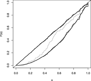
Proceeding similarly for all the 84 experiments and combining the lists $P(y)$ multiplied by 1$/$84 (i.e., the contribution of each experiment to the overall distribution), we obtain the global probability function of the $p$-values, from which the final cumulative distribution is computed (overall there are 14,218 distinct possible $p$-values, but from those the smallest 12,110 were not considered because their cumulative probability is smaller than 0.001). The result is shown in Figure 13. Although for some of the experiments, when considered individually, the c.d.f. of the $p$-values is quite different from that of the uniform $(0,1)$ distribution (like in the example above), when the 84 experiments are taken together the resulting c.d.f. of the $p$-values is very close to the straight line $F(x)=x$, which means that we can safely approximate this distribution by a continuous uniform distribution in $(0,1)$ and trust the results obtained with the K–S test (the approximation is not so good near the upper right corner, but this area is not relevant to this conclusion). The same remarks apply when the exact distribution of the maximum of two $p$-values is approximated by the curve $y=x^{2}$ (see also Figure 6).

B.3 Estimation of the Parameter of Model A

As explained in Section 5.1, we consider the estimate of $\alpha$ defined as the value of $\alpha$ which maximizes the $p$-value of the K–S test for testing the uniformity of the experimental $p$-values, denoted by $p(\alpha)$. The solution can be found by grid search, varying $\alpha$ in a finite set of equidistant points between 0 and 1. With a grid width of 0.001, the value $\hat{\alpha}=0.201$ was obtained. It is also possible (Easterling, 1976) to compute a $100\times\gamma\%$ confidence interval for $\alpha$ by inversion of the K–S test. This confidence interval is the set of points $\alpha\in(0,1)$ such that $\mbox{$p$-value}(\alpha)\geq 1-\gamma$ (it may happen that this confidence set is empty, which is an indication that the model is not appropriate).

A simulation study was performed to validate this procedure. 1000 samples of 84 $p$-values were generated from the 84 binomial experiments, but considering the repetition mechanism of model A with $\alpha=0.2$. For each of those 1000 samples the point estimate and the 90% confidence interval for $\alpha$ were computed as described in the previous paragraph. The results of the simulation confirmed that the whole procedure is adequate and performs as expected: the 1000 point estimates are distributed almost symetrically with mean${}={}$0.2077 ($\mathit{se}=0.0032$), median${}={}$0.194 and standard deviation${}={}$0.101. The confidence set was empty in one case only. From the remaining 999 intervals (mean length${}={}$0.3019, $\mathit{se}=0.0049$; median length${}={}$0.272), 895 contained the true value of $\alpha=0.2$, which gives an estimated confidence level of 89.5%, in close agreement with the specified 90% confidence.

Appendix C The Chi-Square Analysis Assuming Model A

The aim of this note is to show in detail why model A explains the chi-square analysis, and to derive theoretically the approximate distribution of the global chi-square statistic which can be used to compute approximate $p$-values without the need to run simulations.

Fisher’s chi-square analysis is based on the following simple reasoning: Let $X_{i}$, $i=1,\ldots,84$, be the random variable describing the results of the $i$th experiment, that is, the number of observations among $n_{i}$ which are classified into a category of interest (which one of the two categories is the category of interest is not relevant). Let $p_{i}$ be the probability of an observation of that category in a single trial and $p_{i0}$ the value of the same probability according to Mendel’s theory. The standard model is $X_{i}\sim\operatorname{Bin}(n_{i},p_{i})$. If, furthermore, it is assumed, as Fisher did, that the $X_{i}$ are independent and $H_{0i}\dvtx p_{i}=p_{i0}$ is true for all $i=1,\ldots,84$, it follows that

$$X_{1},\ldots,X_{84}\stackrel{{\scriptstyle\mathrm{i.n.d.}}}{{\sim}}\operatorname{Bin}(n_{i},p_{i0})$$

$$\quad\Rightarrow\quad\chi_{i}=\frac{X_{i}-n_{i}p_{i0}}{\sqrt{n_{i}p_{i0}(1-p_{i0})}}\stackrel{{\scriptstyle\mathrm{i.i.d.}}}{{\sim}}_{\!a}N(0,1)$$

$$\quad\Rightarrow\quad Q_{i}=\frac{(X_{i}-n_{i}p_{i0})^{2}}{n_{i}p_{i0}(1-p_{i0})}\stackrel{{\scriptstyle\mathrm{i.i.d.}}}{{\sim}}_{\!a}\chi_{1}^{2}$$

$$\quad\Rightarrow\quad Q_{T}=\sum_{i=1}^{84}Q_{i}\sim_{a}\chi_{84}^{2}.$$

We also have that $E(Q_{T})=84$ and $\operatorname{var}(Q_{T})=168$ [$E(Q_{i})=1$ and $\operatorname{var}(Q_{i})=2$], and $p$-value $=P(Q_{T}>Q_{T\mathrm{\ observed}})=P(Q_{T}>41.3376)\simeq 0.99998$.

From Mendel’s paper we already know that he performed other experiments than the 84 binomial experiments we have been considering. Let us assume that he has (or could have) done $2\times 84=168$ binomial experiments, such that for each of the reported 84 experiments there is a repetition (either actual or conceptual) and denote the repetition of $X_{i}$ by $X_{i+84}$ and the corresponding chi-square statistics by $Q_{i}$ and $Q_{i+84}$. If for each pair ($X_{i},X_{84+i}$) the selection of the reported experiment is random, then the observed statistics, denoted $Q_{i}^{\star}$, $i=1,\ldots,84$, are still i.i.d. $\chi^{2}_{1}$ and Fisher’s analysis remains valid. However, if the selection is not random, and is done according to our model A, we still have that (assuming, as Fisher did, that $X_{i}$ are independent and $H_{0i}$: $p_{i}=p_{i0}$ is true for all $i=1,\ldots,168$)

$$X_{1},\ldots,X_{168}\stackrel{{\scriptstyle\mathrm{i.n.d.}}}{{\sim}}\operatorname{Bin}(n_{i},p_{i0})$$

$$\quad\Rightarrow\quad\chi_{1},\ldots,\chi_{168}\stackrel{{\scriptstyle\mathrm{i.i.d.}}}{{\sim}}_{\!a}N(0,1)$$

$$\quad\Rightarrow\quad Q_{1},\ldots,Q_{168}\stackrel{{\scriptstyle\mathrm{i.i.d.}}}{{\sim}}_{\!a}\chi_{1}^{2},$$

but each of the observed statistics, $Q_{i}^{\star}$, $i=1,\ldots,84$, is no longer randomly chosen between $Q_{i}$ and $Q_{i+84}$, in fact, they are chosen by the following rule,

$$Q_{i}^{\star}=\cases{\displaystyle Q_{i},&if $Q_{i}\leq c_{\alpha}$,\cr\displaystyle\min(Q_{i},Q_{i+84}),&if $Q_{i}>c_{\alpha}$,}$$

where $c_{\alpha}$ is the $1-\alpha$ quantile of the $\chi^{2}_{1}$ distribution. Therefore, the $Q_{i}^{\star}$ are i.i.d. but do not follow the $\chi^{2}_{1}$ distribution, and, in consequence, $Q_{T}^{\star}=\sum_{i=1}^{84}Q_{i}^{\star}$ also does not follow the $\chi^{2}_{84}$ distribution.

The exact distribution of $Q_{T}^{\star}$ appears to be very difficult to derive; however, by the Central Limit Theorem (CLT), we can use a normal approximation,

$$Q_{T}^{\star}\sim_{a}N(84\mu^{\star},84\sigma^{\star 2}),$$

(3)

$$\eqntext{\mbox{with }\mu^{\star}=E(Q_{i}^{\star})\mbox{ and }\sigma^{\star 2}=\operatorname{var}(Q_{i}^{\star}).}$$ (4)

Assuming that $Q_{i}\sim\chi^{2}_{1}$, it is possible to compute the mean and the variance of $Q_{i}^{\star}$, either directly or determining first the pdf of $Q_{i}^{\star}$, $f_{Q^{\star}}$.

Figure 14: Plots of $F^{\ast}_{\alpha}$ when $F_{0}$ is given by (5) for $\alpha=0,0.2,1$, $p_{0}=0.5$ and three combinations of $(n,p_{1})$.

Given the reported value of the statistic, $Q^{\star}_{i}$ according to model A, and the $p$-value computed using the chi-square distribution, given by $P=1-F_{Q_{i}}(Q^{\star}_{i})$, with distribution function given by (1), we have that

$$F_{Q^{\star}}(x) = P(Q^{\star}\leq x)=P\bigl{(}P\geq 1-F_{Q_{i}}(x)\bigr{)}$$

$$= 1-F_{P}\bigl{(}1-F_{Q_{i}}(x)\bigr{)}.$$

Taking derivatives on both sides yields

$$f_{Q^{\star}}(x) = f_{Q_{i}}(x)\frac{dF_{P}(u)}{du}\bigg{|}_{u=1-F_{Q_{i}}(x)}$$

$$= \cases{\displaystyle 2f_{Q_{i}}(x)[1-F_{Q_{i}}(x)],&if $x>c_{\alpha}$,\cr\displaystyle(1+\alpha)f_{Q_{i}}(x),&if $x\leq c_{\alpha}$,}$$

where $f_{Q_{i}}(x)=e^{-x/2}/\sqrt{2\pi x}$, $x>0$, and $F_{Q_{i}}(x)=\int_{0}^{x}f_{Q_{i}}(u)\,du$.

Using symbolic computation, we obtained $\mu^{\star}=1-(2k_{\alpha}+(1-\alpha)\sqrt{2c_{\alpha}k_{\alpha}})$, $\sigma^{\star 2}=2-(4k_{\alpha}^{2}+(1-\alpha)\sqrt{2c_{\alpha}k_{\alpha}}(4k_{\alpha}+1+c_{\alpha})+2(2+c_{\alpha}(2-2\alpha+\alpha^{2}))k_{\alpha})$, with $k_{\alpha}=e^{-c_{\alpha}}/\pi$. Table 10 gives the values of $\mu^{\star}$ and $\sigma^{\star 2}$, as well as the $p$-values obtained using the normal approximation (C), for the three values of $\alpha$ considered previously. The $p$-values obtained in the simulation study (see Table 6) are also provided for comparison. The two columns of $p$-values are very similar. The results presented in this appendix are thus an independent validation of the simulation results, in case there was any doubt about them.

Table 10: Mean and variance of $Q_{i}^{\star}$ and $p$-values obtained using the normal approximation to $Q_{T}^{\ast}$ and from the Monte Carlo simulation

				$\bolds p$-value	$\bolds p$-value
$\bolds\alpha$	$\bolds{c_{\alpha}}$	$\bolds{\mu^{\ast}}$	$\bolds{\sigma^{\star 2}}$	(normal approx.)	(simulation)
0.094	2.805	0.6636	0.5685	0.9814	0.9860
0.201	1.635	0.5160	0.3662	0.6412	0.6577
0.362	0.831	0.4164	0.3135	0.1076	0.1176

Appendix D Model A for an Incorrect Theory

Suppose that Mendel’s theory was not right but that the same selection mechanism was applied (i.e., an experiment was repeated whenever its $p$-value was smaller than $\alpha$, $0\leq\alpha\leq 1$, and then only the experiment with the largest $p$-value was reported). The difference between this case and that one considered in Section 5.1 is that the original distribution of the $p$-values is not uniform $(0,1)$ but has a c.d.f. $F_{0}(x)\neq x$ for some $0<x<1$. Then, proceeding as in the proof of (1), we can conclude that the $p$-values effectively reported have a c.d.f. given by

$$F^{\ast}_{\alpha}(x)=\cases{\displaystyle[F_{0}(x)]^{2},\cr\quad\mbox{if }0\leq x\leq\alpha,\cr\displaystyle[1+F_{0}(\alpha)]F_{0}(x)-F_{0}(\alpha),\cr\quad\mbox{if }\alpha<x\leq 1.}$$

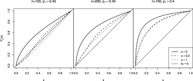
The selection procedure would make an incorrect theory look correct if $F^{\ast}_{\alpha}(x)$ is “close” to the c.d.f. of a uniform $(0,1)$ random variable. The result depends on the starting point, $F_{0}(x)$, which in turn depends on the particular test under analysis and on the true and hypothesized parameters, as the following example shows.

Suppose that the theory states that the success probability of a binomial random variable is $p_{0}$ but that data are actually observed from a binomial random variable with success probability $p_{1}$ which may be different from $p_{0}$. Assuming that $n$ is large, the normal approximation to the binomial leads to

$$F_{0}(x)=\Phi\biggl{(}\frac{-z-\delta}{\eta}\biggr{)}+1-\Phi\biggl{(}\frac{z-\delta}{\eta}\biggr{)},$$ (5)

where $\Phi(x)$ is the c.d.f. of a standard normal random variable, $z=\Phi^{-1}(1-x/2)$,

$$\delta=\frac{n(p_{1}-p_{0})}{\sqrt{np_{0}(1-p_{0})}}\quad\mbox{and}\quad\eta^{2}=\frac{p_{1}(1-p_{1})}{p_{0}(1-p_{0})}.$$

Note that, when $p_{0}=p_{1}$, $F_{0}(x)\equiv x$, as it should.

Figure 14 shows the results for $p_{0}=1/2$ and some values of $n$, $p_{1}$ and $\alpha$. We conclude that in the first case ($n=100$, $p_{1}=0.45$) it is easy to make the theory look correct, but as $n$ increases or $p_{1}$ deviates from $p_{0}$ that becomes more difficult.

There is, of course, the possibility of further generalizing model A by making more than 2 repetitions per experiment, say, $k$. With this extra flexibility it is easy to make any theory look correct.

References

- Bateson (1902) Bateson, W. (1902). Mendel’s Principles of Heredity, a Defense, 1st ed. Cambridge Univ. Press, London.
- Bateson (1909) Bateson, W. (1909). Mendel’s Principles of Heredity, a Defense, 2nd ed. Cambridge Univ. Press, London.
- Bowler (1989) Bowler, P. J. (1989). The Mendelian Revolution. Athlone, London.
- Dawkins (1995) Dawkins, R. (1995). River out of Eden: A Darwinian View of Life. Perseus Books Group, New York.
- De Beer (1964) De Beer, G. (1964). Mendel, Darwin and Fisher (1865–1965). Notes and Records Roy. Soc. London 19 192–226.
- Di Trocchio (1991) Di Trocchio, F. (1991). Mendel’s experiments: A reinterpretation. J. Hist. Biol. 24 485–519.
- Dobzhansky (1967) Dobzhansky, T. (1967). Looking back at Mendel’s discovery. Science 156 1588–1589.
- Easterling (1976) Easterling, R. G. (1976). Goodness of fit and parameter estimation. Technometrics 18 1–9.
- Edwards (1986a) Edwards, A. W. F. (1986a). Are Mendel’s results really too close? Biol. Rev. 61 295–312. Also reproduced in Franklin et al. (2008).
- Edwards (1986b) Edwards, A. W. F. (1986b). More on the too-good-to-be true paradox and Gregor Mendel. J. Hered. 77 138.
- Fairbanks and Rytting (2001) Fairbanks, D. J. and Rytting, B. (2001). Mendelian controversies: A botanical and historical review. Am. J. Bot. 88 737–752. [Also reproduced in Franklin et al. (2008).]
- Fairbanks and Schaalje (2007) Fairbanks, D. J. and Schaalje, B. (2007). The tetrad-pollen model fails to explain the bias in Mendel’s pea (Pisum sativum) experiments. Genetics 177 2531–2534.
- Fisher (1936) Fisher, R. A. (1936). Has Mendel’s work been rediscovered? Ann. of Sci. 1 115–137. [Also reproduced in Franklin et al. (2008).]
- Franklin et al. (2008) Franklin, A., Edwards, A. W. F., Fairbanks, D. J., Hartl, D. L. and Seidenfeld T. (2008). Ending the Mendel–Fisher Controversy. Univ. Pittsburgh Press, Pittsburgh.
- Hald (1998) Hald, A. (1998). A History of Mathematical Statistics. Wiley, New York. \MR1619032
- Hartl and Fairbanks (2007) Hartl, D. L. and Fairbanks, D. J. (2007). Mud sticks: On the alleged falsification of Mendel’s data. Genetics 175 975–979.
- Leonard (1977) Leonard, T. (1977). A Bayesian approach to some multinomial estimation and pretesting problems. J. Amer. Statist. Assoc. 72 869–874. \MR0652717
- Massey (1951) Massey, F. J. (1951). The Kolmogorov–Smirnov test for goodness of fit. J. Amer. Statist. Assoc. 46 68–78.
- Meijer (1983) Meijer, O. (1983). The essence of Mendel’s discovery. In Gregor Mendel and the Foundation of Genetics (V. Orel and A. Matalová, eds.) 123–172. Mendelianum of the Moravian Museum, Brno, Czechoslovakia.
- Mendel (1866) Mendel, G. (1866). Versuche über plflanzenhybriden verhandlungen des naturforschenden vereines in Brünn. In Bd. IV für das Jahr, 1865 78–116. [The first english translation, entitled “Experiments in plant hybridization,” published in Bateson (1909) is also reproduced in Franklin et al. (2008).]
- Nissani and Hoefler-Nissani (1992) Nissani, M. and Hoefler-Nissani, D. M. (1992). Experimental studies of belief-dependence of observations and of resistance to conceptual change. Cognition Instruct. 9 97–111.
- Novitski (1995) Novitski, C. E. (1995). Another look at some of Mendel’s results. J. Hered. 86 62–66.
- Olby (1984) Olby, R. (1984). Origin of Mendelism, 2nd ed. Univ. Chicago Press, Chicago.
- Pearson (1900) Pearson, K. (1900). On the criterion that a given system of deviations from the probable in the case of a correlated system of variables is such that it can be reasonably supposed to have arised from random sampling. Philos. Mag. 50 157–175.
- Piegorsch (1983) Piegorsch, W. W. (1983). The questions of fit in the Gregor Mendel controversy. Comm. Statist. Theory Methods 12 2289–2304.
- Pilgrim (1984) Pilgrim, I. (1984). The too-good-to-be-true paradox and Gregor Mendel. J. Hered. 75 501–502.
- Pilgrim (1986) Pilgrim, I. (1986). A solution to the too-good-to-be-true paradox and Gregor Mendel. J. Hered. 77 218–220.
- R Development Core Team (2008) R Development Core Team (2008). R: A Language and Environment for Statistical Computing. R Foundation for Statistical Computing, Vienna, Austria.
- Robertson (1978) Robertson, T. (1978). Testing for and against an order restriction on multinomial parameters. J. Amer. Statist. Assoc. 73 197–202. \MR0488300
- Root-Bernstein (1983) Root-Bernstein, R. S. (1983). Mendel and methodology. Hist. Sci. 21 275–295.
- Rosenthal (1976) Rosenthal, R. (1976). Experimenter Effects in Behavioural Research. Irvington, New York.
- Seidenfeld (1998) Seidenfeld, T. (1998). P’s in a pod: Some recipes for cooking Mendel’s data. PhilSci Archive, Department of History and Philosophy of Science and Department of Philosophy, Univ. Pittsburgh. [Also reproduced in Franklin et al. (2008).]
- Stigler (2008) Stigler, S. M. (2008). CSI: Mendel. Book review. Am. Sci. 96 425–426.
- Thagard (1988) Thagard, P. (1988). Computational Philosophy of Science. MIT Press, Cambridge, MA. \MR0950373
- Weiling (1986) Weiling, F. (1986). What about R.A. Fisher’s statement of the “Too Good” data of J. G. Mendel’s Pisum paper? J. Hered. 77 281–283.
- Weldon (1902) Weldon, W. R. F. (1902). Mendel’s law of alternative inheritance in peas. Biometrika 1 228–254.