Equilibrium Statistics of Weakly Slip-Linked Gaussian Polymer Chains

TAKASHI UNEYAMA^1,2, KAZUSHI HORIO¹

¹ Institute for Chemical Research, Kyoto University, Gokasho, Uji, Kyoto 611-0011, JAPAN
² JST-CREST, Gokasho, Uji, Kyoto 611-0011, JAPAN

Dated:

INTRODUCTION

The motion of polymer chains in melts or solutions are strongly constrained due to the entanglement effect¹, if the degrees of polymerization are large. Although the entanglement affects dynamic properties drastically, it does not affect the static properties. For example, in polymer melts, conformations of polymer chains are well described by the ideal, Gaussian statistics² beyond a certain length scale. Therefore, if we are interested only on static properties, the Gaussian chain model can be reasonably utilized. Actually theories based on the Gaussian statistics achieved great success to predict static phase behaviours of polymer blends or block copolymers^{3, 4, 5}. However, once we consider dynamics of entangled chains, the situation becomes complicated so much.

It is informative to consider simple toy models which show non-trivial dynamical behaviours due to topological constraints. It was reported that molecules composed of infinitely thin rods exhibit glass transition by increasing the density^{6, 7, 8}, while thermodynamically they are ideal gases. The situation is almost the same for entangled polymers. The entanglement effects exist even for ideal chains as long as they cannot cross each other. (Although interactions between monomers or between monomer and solvent alter rheological behaviours somehow, such effects are secondary.) Unfortunately, it is not easy to treat such dynamic effects theoretically. Thus several phenomenological models such as the tube model¹ or the slip-link model⁹ have been proposed and utilized. The slip-link model represent an entanglement as a linking point on polymers which can slide along the chains (slip-links). So far, various slip-link type models^{9, 10, 11, 12, 13, 14} have been utilized to study rheological properties of entangled polymers, and slip-link models have reproduced various rheological properties well.

However, it is reported that the slip-link models can exhibit unintuitive statistics in several situations^{15, 16, 17, 18, 19, 20, 21}. The simplest example is the statistics of a single Gaussian chain with slip-links. Rieger^{15, 16, 17} calculated the partition function of a Gaussian chain with a slip-link and showed that this system can exhibit spontaneous symmetry breaking and bifurcation. Metzler, Kardar and co workers^{19, 20, 21} studied a single ring polymer with slip-links as a model of a knotted ring polymer, and found that slip-linked portion localizes on a ring. This is similar to Rieger’s results. They reported that the localization behaviour is observed even in presence of the excluded volume interaction. Sommer¹⁸ studied two chains bound by a slip-link, and found similar unintuitive behaviours. He also found that when multiple chains are bound by multiple slip-links, slip-links can form compact aggregated structures. These results imply that various slip-link models may exhibit unphysical results.

We consider that macroscopic statistical properties of slip-linked chains may be affected by slip-links. This can be serious problems when we utilize slip-link models to study various macroscopic properties (such as pressure or rheology). As far as the authors know, so far studies for such unintuitive statistics are limited for simple systems such as single chain systems. How slip-links affect macroscopic thermodynamic properties is not clear. In principle, if the statistics of the system is explicitly specified (if the equilibrium probability distribution is explicitly given), we can check whether the macroscopic thermodynamic properties are really affected or not. For example, in single chain slip-link models with the mean filed type approximation^{10, 14} or in virtually coupled many chain slip-link models²², we can straightforwardly show that there are no unintuitive behaviors (as discussed in Appendix A).

The situation is not simple when we consider multi chain slip-link models¹². In this work we consider statistics of weakly slip-linked multi polymer chains theoretically. We calculate the partition function of weakly slip-linked Gaussian chains by utilizing the grand canonical ensemble type treatment developed by Schieber¹⁰. We show that we can calculate the explicit forms of partition function and free energy as perturbation expansions. The free energy of weakly slip-linked chains are shown to be different from one for ideal chains without any constraints by slip-links. We also show that slip-links decrease the pressure, and thus repulsive interactions between chains are required for such systems to recover (or mimic) the ideal statistics.

THEORY

Thermodynamic Equilibrium Distribution of Gaussian Chains

Before we calculate the partition function for slip-linked chains, we first consider the partition function of Gaussian chains without any constraints by slip-links. (We call such systems as “the ideal chain systems” or “the ideal systems”, in the followings.) As we mentioned, even if chains are well entangled, equilibrium statistical properties can be well described by the Gaussian chain model since the entanglement effect is purely kinetic. As pointed simply by Doi²³, the entanglement effects exist even for ideal chains without excluded volume effects. Therefore we limit ourselves to ideal chains and ignore interaction potentials between monomers although they may not be negligible for some cases (especially for small length scales). Thus the partition function or the free energy for ideal chains can be directly applied both to unentangled or entangled polymers. Although one may consider this is an oversimplification, as we will show in the followings, we can still obtain nontrivial results for slip-linked chains. We will compare the results of this subsection with the statistics of slip-linked chains later.

Some expressions in this subsection can be utilized in the next subsection, to calculate the partition function for slip-linked chains. Thus here we calculate the partition function for Gaussian chains rather verbosely. It is convenient to start from a single chain partition function, since the partition function of the system can be easily calculated from the single chain partition function in non-interacting multi chain systems. We describe the conformation of a polymer chain as $\bm{R}(s)$ ($0\leq s\leq N$). $s$ is the index along the chain and $N$ is the degree of polymerization. The single chain partition function without any constraints can be formally described by using the Edwards Hamiltonian and the functional integral expression.

$$\mathcal{Z}_{1}\equiv\int\mathcal{D}\bm{R}\,\exp\left[-\frac{\mathcal{H}_{0}[\bm{R}(\cdot)]}{k_{B}T}\right]$$ (1)

where $\mathcal{H}_{0}[\bm{R}(\cdot)]$ is the Edwards Hamiltonian and $\int\mathcal{D}\bm{R}$ means the functional integral over $\bm{R}$. We assume that the functional integral $\int\mathcal{D}\bm{R}$ contains an appropriate measure so that the resulting functional integral becomes dimensionless. The subscript $1$ in the left hand side of eq (1) indicates that it is the partition function for a single chain. The Edwards Hamiltonian for a Gaussian chain is expressed as

$$\mathcal{H}_{0}[\bm{R}(\cdot)]=\frac{3k_{B}T}{2b^{2}}\int_{0}^{N}ds\,\left|\frac{\partial\bm{R}(s)}{\partial s}\right|^{2}$$ (2)

Here $k_{B}$ is the Boltzmann constant, $T$ is the temperature, and $b$ is the segment size. (As we mentioned, the interaction between monomers are not considered in this work and thus we have no interaction energy in eq (2).)

We introduce the constraint which fixes the position of the chain at the index $s_{1}$, $\bm{R}(s_{1})$, to $\bm{r}_{1}$. From translational symmetry (translational invariance), the partition function under this constraint is independent of $s_{1}$ and $\bm{r}_{1}$. Then we can define the following partition function.

$$\mathcal{Q}\equiv\int\mathcal{D}\bm{R}\,\left[\Lambda^{3}\delta(\bm{r}_{1}-\bm{R}(s_{1}))\right]\exp\left[-\frac{\mathcal{H}_{0}[\bm{R}(\cdot)]}{k_{B}T}\right]$$ (3)

Here we introduced the dimensional factor $\Lambda^{3}$ (with $\Lambda$ being the thermal de Broglie wave length of the chain) to make the partition function dimensionless. Eq (3) corresponds to the partition function for the internal degrees of freedom. By using eq (3), the single chain partition function (1) can be rewritten as

$$\mathcal{Z}_{1}=\frac{1}{N\Lambda^{3}}\int_{0}^{N}ds_{1}\int d\bm{r}_{1}\,\mathcal{Q}=\frac{V\mathcal{Q}}{\Lambda^{3}}$$ (4)

where $V$ is the system volume.

Next we consider a canonical ensemble of Gaussian chains. The partition function for $M$ Gaussian chains can be simply written as follows, by using the single chain partition function (4).

$$\mathcal{Z}^{(0)}=\frac{\mathcal{Z}_{1}^{M}}{M!}=\frac{V^{M}\mathcal{Q}^{M}}{M!\Lambda^{3M}}$$ (5)

The superscript $(0)$ is used to indicate an ideal system. The free energy of the system is simply calculated to be

$$\mathcal{F}^{(0)}=-k_{B}T\ln\mathcal{Z}^{(0)}=k_{B}TM\left[\ln\frac{M\Lambda^{3}}{V\mathcal{Q}}-1\right]$$ (6)

Thus the pressure becomes as follows.

$$P^{(0)}=-\frac{\partial\mathcal{F}^{(0)}}{\partial V}=\frac{k_{B}TM}{V}$$ (7)

This is nothing but the standard van’t Hoff form (the equation of state for ideal gas). The pressure is simply proportional to the polymer chain density $M/V$. We again emphasize that eq (7) holds even if chains are entangled, because the entanglement effect is purely kinetic. Although results shown here are rather trivial, it is not trivial whether the slip-linked chains have the same statistics or not. In the following sections, we calculate the static thermodynamic properties of slip-linked chains.

Partition Function of Slip-Linked Chain Clusters

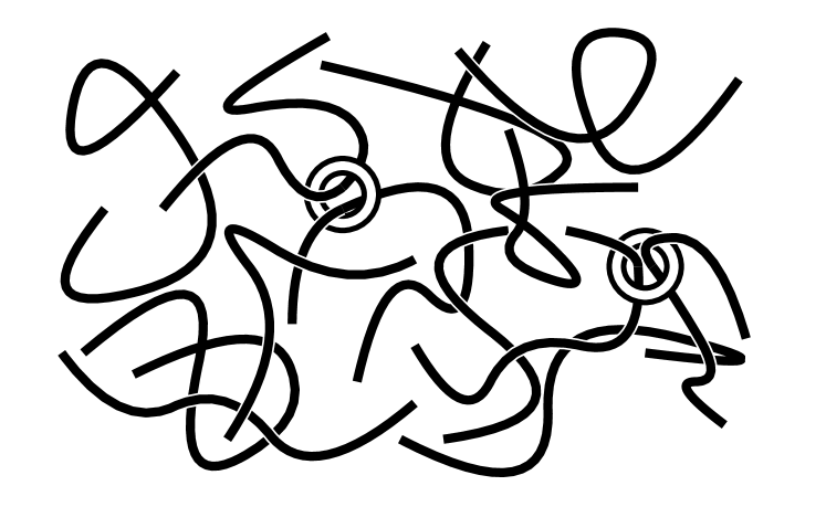
Figure 1: An image of a weakly slip-linked multi chain system. Black curves and white circles represent polymer chains and slip-links. Only a small fraction of chains are constrained by slip-links.

We consider weakly slip-linked chains in this and following subsections. For simplicity, we assume that slip-links do not interact each other, and a single slip-link always bind two chain portions in space. Under the constraints by slip-links, the thermodynamic properties of the system will be altered. It can be shown by calculating the partition function for a slip-linked chains. If we assume that the constraints by slip-links are sufficiently weak (or chains are sufficiently short), it is justified to neglect complicated network like structures with many slip-links. We show an image of a weakly slip-linked multi chain system in Figure 1. Then we need to calculate only several simple slip-linked structures, to obtain the expression of the partition function of the system. This is similar to the case of weakly interacting real gas²⁴. If the interaction between gas molecules is sufficiently weak, we only need several lower order Mayer clusters to study thermodynamic properties.

The most simple slip-linked structure is two chains paired by one slip-link. The schematic image of a chain-pair is depicted in Figure 2(a). We may call such a structure as a “slip-linked chain cluster” or simply a “cluster”, in analogy to the Mayer clusters. It is easy to show that the expression for the partition function is different from the ideal case. The partition function can be calculated straightforwardly by imposing the slip-linking effect by a delta function. We express the conformations of two chains by $\bm{R}_{1}(s)$ and $\bm{R}_{2}(s)$. Two points on these chains, $\bm{R}_{1}(s_{1})$ and $\bm{R}_{2}(s_{2})$ are coupled by a slip-link ($s_{1}$ and $s_{2}$ are indices of slip-linked points). The partition function is calculated as follows.

$$\begin{split}\mathcal{Z}_{2(1,1)}&=\frac{1}{2!N^{2}\Lambda^{6}}\int\mathcal{D}\bm{R}_{1}\mathcal{D}\bm{R}_{2}\int ds_{1}ds_{2}\,[\Lambda^{3}\delta(\bm{R}_{1}(s_{1})-\bm{R}_{2}(s_{2}))]\\ &\qquad\times\exp\left[-\frac{\mathcal{H}_{0}[\bm{R}_{1}(\cdot)]+\mathcal{H}_{0}[\bm{R}_{1}(\cdot)]}{k_{B}T}\right]\\ &=\frac{\mathcal{Q}^{2}}{2!N^{2}\Lambda^{6}}\int_{0}^{N}ds_{1}\int_{0}^{N}ds_{2}\int d\bm{r}_{1}d\bm{r}_{2}\,[\Lambda^{3}\delta(\bm{r}_{1}-\bm{r}_{2})]\\ &=\frac{V\mathcal{Q}^{2}}{2\Lambda^{3}}\end{split}$$ (8)

where we introduced the subscript $2(1,1)$ which indicates that the cluster is composed of two chains and each chain has one slip-linked point.

If there are two slip-links, more complicated slip-linked structures can be formed. In this case, there are three different possible cluster structures (Figure 2(b)-(d)). The cluster shown in Figure 2(b) is composed by three chains. The clusters shown in 2(c) and (d) are composed by two chains, but their topologies are different. After straightforward calculations, we have the following partition functions for these clusters.

$$\mathcal{Z}_{3(1,1,2)}=\frac{V\mathcal{Q}^{3}}{6\Lambda^{3}}$$ (9)

$$\begin{split}\mathcal{Z}_{2(1,3)}&=\frac{\mathcal{Q}^{2}}{2N^{3}\Lambda^{9}}\int d\bm{r}_{1}d\bm{r}_{2}d\bm{r}_{3}\int_{0}^{N}ds_{1}\int_{s_{1}}^{N}ds_{2}\int_{s_{2}}^{N}ds_{3}\,\left(\frac{3\Lambda^{2}}{2\pi b^{2}}\right)^{3}\frac{1}{[(s_{3}-s_{2})(s_{2}-s_{1})]^{3/2}}\\ &\qquad\times\exp\left[-\frac{3(\bm{r}_{2}-\bm{r}_{1})^{2}}{2(s_{2}-s_{1})b^{2}}-\frac{3(\bm{r}_{3}-\bm{r}_{2})^{2}}{2(s_{3}-s_{2})b^{2}}\right]\Lambda^{3}\delta(\bm{r}_{3}-\bm{r}_{1})\\ &=\frac{2V\mathcal{Q}^{2}}{3\Lambda^{3}}\left(\frac{3\Lambda^{2}}{2\pi Nb^{2}}\right)^{3/2}\end{split}$$ (10)

$$\begin{split}\mathcal{Z}_{2(2,2)}&=\frac{\mathcal{Q}^{2}}{2N^{4}\Lambda^{12}}\int d\bm{r}_{1}d\bm{r}_{2}d\bm{r}_{3}d\bm{r}_{4}\int_{0}^{N}ds_{1}\int_{s_{1}}^{N}ds_{2}\int_{0}^{N}ds_{3}\int_{s_{3}}^{N}ds_{4}\,\left(\frac{3\Lambda^{2}}{2\pi b^{2}}\right)^{3}\\ &\qquad\times\frac{1}{[(s_{4}-s_{3})(s_{2}-s_{1})]^{3/2}}\exp\left[-\frac{3(\bm{r}_{2}-\bm{r}_{1})^{2}}{2(s_{2}-s_{1})b^{2}}-\frac{3(\bm{r}_{4}-\bm{r}_{3})^{2}}{2(s_{4}-s_{3})b^{2}}\right]\\ &\qquad\times\Lambda^{6}\left[\delta(\bm{r}_{3}-\bm{r}_{1})\delta(\bm{r}_{4}-\bm{r}_{2})+\delta(\bm{r}_{4}-\bm{r}_{1})\delta(\bm{r}_{3}-\bm{r}_{2})\right]\\ &=\frac{16(7-4\sqrt{2})}{15}\frac{V\mathcal{Q}^{2}}{\Lambda^{3}}\left(\frac{3\Lambda^{2}}{2\pi Nb^{2}}\right)^{3/2}\\ \end{split}$$ (11)

The subscripts $3(1,1,2)$, $2(1,3)$ or $2(2,2)$ indicate the number of chains and slip-links on each chain, as before. For example, The cluster $3(1,1,2)$ is composed by three chains and they have $1$, $1$, and $2$ slip-linked points.

There are other clusters which are composed of one or two slip-links. As discussed in Appendix B, these clusters have self-slip-linked structures and such self-slip-linked clusters have no effect on static thermodynamical properties. Intuitively, we can understand this as follows. In the self-slip-linked structures, slip-linked portions strongly localize^{19, 20, 21}. Then the partition function for a self-slip-linked structure is almost the same as the partition function for a structure without self-slip-links. Thus such clusters practically do not contribute to the partition function. Anyway, we do not need to consider them when we calculate the partition function of slip-linked chains. All the clusters considered in this subsection are non self-slip-linked clusters and contribute to thermodynamic properties.

Equilibrium Free Energy for Weakly Slip-Linked Chains

We can calculate the partition function of the system from partition functions for clusters (8)-(11). We start from a nearly ideal multi chain system where only small fraction of chains forms slip-linked clusters. Under such a condition, the system partition function can be calculated only by using the partition functions for a free chain and a cluster $2(1,1)$.

According to the Schieber’s theory¹⁰, the distribution of slip-links can be regarded as a sort of ideal gas in a grand canonical ensemble, and they are controlled by the effective chemical potential for slip-links. Then the partition function of the system can be described as

$$\mathcal{Z}\equiv\sum_{M_{1}+2M_{2}=M}\frac{1}{M_{1}!M_{2}!}\exp\left(\frac{\epsilon M_{2}}{k_{B}T}\right)\mathcal{Z}_{1}^{M_{1}}\mathcal{Z}_{2(1,1)}^{M_{2}}$$ (12)

where $M$ is the total number of chains in the system and $\epsilon$ is the effective chemical potential for a slip-link. The sum in eq (12) is taken for $M_{1}$ and $M_{2}$ under the constraint $M_{1}+2M_{2}=M$. The calculation becomes easier if we consider a grand canonical ensemble of chains, instead of a canonical ensemble. If we introduce the chemical potential for a chain, $\mu$, the grand partition function becomes

$$\Xi\equiv\sum_{M_{1}=0}^{\infty}\sum_{M_{2}=0}^{\infty}\frac{1}{M_{1}!M_{2}!}\exp\left[\frac{\mu(M_{1}+2M_{2})}{k_{B}T}+\frac{\epsilon M_{2}}{k_{B}T}\right]\mathcal{Z}_{1}^{M_{1}}\mathcal{Z}_{2(1,1)}^{M_{2}}$$ (13)

Eq (13) can be easily calculated.

$$\begin{split}\Xi&=\exp\left[e^{\mu/k_{B}T}\mathcal{Z}_{1}+e^{(2\mu+\epsilon)/k_{B}T}\mathcal{Z}_{2(1,1)}\right]\\ &=\exp\left[\frac{V\mathcal{Q}}{\Lambda^{3}}e^{\mu/k_{B}T}\left[1+\frac{1}{2}e^{(\mu+\epsilon)/k_{B}T}\mathcal{Q}\right]\right]\end{split}$$ (14)

Thus we obtain the following expression for the grand potential $\mathcal{J}$.

$$\begin{split}\mathcal{J}&\equiv-k_{B}T\ln\Xi\\ &=-k_{B}T\frac{V\mathcal{Q}}{\Lambda^{3}}e^{\mu/k_{B}T}\left[1+\frac{1}{2}e^{(\mu+\epsilon)/k_{B}T}\mathcal{Q}\right]\end{split}$$ (15)

Now we can calculate the free energy by using the Legendre transform.

$$M=-\frac{\partial\mathcal{J}}{\partial\mu}=\frac{V\mathcal{Q}}{\Lambda^{3}}e^{\mu/k_{B}T}\left[1+e^{(\mu+\epsilon)/k_{B}T}\mathcal{Q}\right]$$ (16)

$$\begin{split}\mathcal{F}&=\mathcal{J}+\mu M\\ &=-\frac{1}{2}k_{B}TM-\frac{1}{2}k_{B}TM\left[\frac{1}{2}\sqrt{1+4e^{\epsilon/k_{B}T}\frac{M\Lambda^{3}}{V}}+\frac{1}{2}\right]^{-1}\\ &\qquad-\epsilon M+k_{B}TM\ln\left[\frac{1}{2}\sqrt{1+4e^{\epsilon/k_{B}T}\frac{M\Lambda^{3}}{V}}-\frac{1}{2}\right]-k_{B}T\ln\mathcal{Q}\end{split}$$ (17)

The pressure of the system is calculated to be

$$P=-\frac{\partial\mathcal{F}}{\partial V}=\frac{k_{B}TM}{2V}\Bigg{[}1+\left[\frac{1}{2}\sqrt{1+4e^{\epsilon/k_{B}T}\frac{M\Lambda^{3}}{V}}+\frac{1}{2}\right]^{-1}\Bigg{]}$$ (18)

Clearly the free energy (17) and the pressure (18) are different from ones for an ideal system (eqs (6) (7))

It is convenient to introduce the average number of slip-linked points on a chain, $\tilde{Z}$. The average number of slip-linked points (entanglements) on a chain can be calculated directly from the free energy.

$$\tilde{Z}=-\frac{2}{M}\frac{\partial\mathcal{F}}{\partial\epsilon}=1-\left[\frac{1}{2}\sqrt{1+4e^{\epsilon/k_{B}T}\frac{M\Lambda^{3}}{V}}+\frac{1}{2}\right]^{-1}$$ (19)

Here the factor $2$ is introduced because one slip-link corresponds to two entanglement points (see Figure 2). From eq (19) we find that the average number of slip-links on a chain depends on the polymer chain density $M/V$. We can modify eq (19) and obtain the following relation.

$$4e^{\epsilon/k_{B}T}\frac{M\Lambda^{3}}{V}=\bigg{(}\frac{1+\tilde{Z}}{1-\tilde{Z}}\bigg{)}^{2}-1$$ (20)

Eq (20) gives the relation among the effective chemical potential, the chain number density, and the number of slip-links on a chain. Since we are considering weakly slip-linked chains, the number of slip-linked points on a chain should be sufficiently small ($\tilde{Z}\ll 1$) and thermodynamic quantities can be expanded into power series of $\tilde{Z}$ around $\tilde{Z}=0$. The power series expressions will help us to interpret the physical meanings of the results. Eq (20) can be expanded as follows.

$$e^{\epsilon/k_{B}T}\frac{M\Lambda^{3}}{V}=\tilde{Z}+O(\tilde{Z}^{2})$$ (21)

By using (21), we can rewrite the free energy (17) and the pressure (18) simply as follows.

$$\mathcal{F}=k_{B}TM\left[\ln\frac{M\Lambda^{3}}{V\mathcal{Q}}-1\right]-\frac{1}{2}k_{B}TM\tilde{Z}+O(\tilde{Z}^{2})\\$$ (22)

$$P=\frac{k_{B}TM}{V}-\frac{1}{2}\frac{k_{B}TM}{V}\tilde{Z}+O(\tilde{Z}^{2})$$ (23)

It is now clear that eqs (22) and (23) reduces to eqs (6) and (7), respectively, at the limit of $\tilde{Z}\to 0$. We can rewrite eqs (22) and (23) as follows by using eqs (6) and (7).

$$\mathcal{F}-\mathcal{F}^{(0)}=-\frac{1}{2}k_{B}TM\tilde{Z}+O(\tilde{Z}^{2})$$ (24)

$$P-P^{(0)}=-\frac{1}{2}\frac{k_{B}TM}{V}\tilde{Z}+O(\tilde{Z}^{2})$$ (25)

Eqs (24) and (25) give the expressions for the excess free energy and the excess pressure. From eq (24) we find that the system free energy is decreased by slip-links. Eq (25) means that the pressure of a weakly slip-linked chain system becomes slightly lower than the pressure of the corresponding ideal chain system. A weakly slip-linked system does not obey the equation of state for an ideal gas.

Effect of Higher Order Clusters

In the previous subsection, we have considered only the first order cluster. In this subsection we consider the effect of the higher order clusters. If we retain the clusters up to the second order, the expression for the grand potential becomes

$$\begin{split}\mathcal{J}&=-k_{B}T\bigg{[}e^{\mu/k_{B}T}\mathcal{Z}_{1}+e^{(2\mu+\epsilon)/k_{B}T}\mathcal{Z}_{2(1,1)}+e^{(3\mu+2\epsilon)/k_{B}T}\mathcal{Z}_{3(1,1,1)}\\ &\qquad+e^{(2\mu+2\epsilon)/k_{B}T}\mathcal{Z}_{2(1,3)}+e^{(2\mu+2\epsilon)/k_{B}T}\mathcal{Z}_{2(2,2)}\bigg{]}\\ &=-k_{B}Te^{\mu/k_{B}T}\frac{V\mathcal{Q}}{\Lambda^{3}}\bigg{[}1+\frac{1}{2}e^{(\mu+\epsilon)/k_{B}T}\mathcal{Q}+\frac{1}{6}e^{(2\mu+2\epsilon)/k_{B}T}\mathcal{Q}^{2}\\ &\qquad+\frac{2(61-32\sqrt{2})}{15}e^{(\mu+2\epsilon)/k_{B}T}\mathcal{Q}\left(\frac{3\Lambda^{2}}{2\pi Nb^{2}}\right)^{3/2}\bigg{]}\end{split}$$ (26)

From the results of the previous subsection, we expect that $\xi\equiv e^{(\epsilon+\mu)/k_{B}T}\mathcal{Q}$ becomes a small perturbation parameter which represents the strength of constraints by slip-links. ($\xi$ may be interpreted as the effective fugacity for slip-links. $\xi=0$ corresponds to a non slip-linked, free ideal chain system.) Then thermodynamic quantities can be expanded into power series of $\xi$ around $\xi=0$. Since all the clusters which contain two or less slip-links are included in eq (26), we can calculate the expansion up to $O(\xi^{2})$. From eq (21) we find that $O(\tilde{Z})=O(\xi)$, and thus we can calculate the expansion series up to $O(\tilde{Z}^{2})$.

The number of chains in the system is calculated to be

$$M=e^{\mu/k_{B}T}\frac{V\mathcal{Q}}{\Lambda^{3}}\bigg{[}1+\xi+\frac{1}{2}\xi^{2}+\frac{4(61-32\sqrt{2})}{15}\xi^{2}\frac{e^{-\mu/k_{B}T}}{\mathcal{Q}}\left(\frac{3\Lambda^{2}}{2\pi Nb^{2}}\right)^{3/2}\bigg{]}$$ (27)

Then the chemical potential can be related to $M$ and $\xi$ as follows.

$$\begin{split}\mu&=k_{B}T\ln\frac{M\Lambda^{3}}{V\mathcal{Q}}-k_{B}T\bigg{[}\xi+\frac{4(61-32\sqrt{2})}{15}\xi^{2}\frac{V}{M}\left(\frac{3}{2\pi Nb^{2}}\right)^{3/2}+O(\xi^{3})\bigg{]}\end{split}$$ (28)

After the straightforward calculations, we have the following expressions for the grand partition function or the free energy.

$$\mathcal{J}=-k_{B}TM\bigg{[}1-\frac{1}{2}\xi+\frac{2}{3}\xi^{2}-\frac{2(61-32\sqrt{2})}{15}\xi^{2}\frac{V}{M}\left(\frac{3}{2\pi Nb^{2}}\right)^{3/2}+O(\xi^{3})\bigg{]}$$ (29)

$$\mathcal{F}=\mathcal{F}^{(0)}-k_{B}TM\bigg{[}\frac{1}{2}{\xi}+\frac{2}{3}\xi^{2}+\frac{2(33-16\sqrt{2})}{15}\xi^{2}\frac{V}{M}\left(\frac{3}{2\pi Nb^{2}}\right)^{3/2}+O(\xi^{3})\bigg{]}$$ (30)

The pressure can be obtained from eq (30).

$$P=P^{(0)}-k_{B}T\bigg{[}\frac{1}{2}\xi\frac{M}{V}+\frac{4}{3}\xi^{2}\frac{M}{V}+\frac{2(61-32\sqrt{2})}{15}\xi^{2}\left(\frac{3}{2\pi Nb^{2}}\right)^{3/2}+O(\xi^{3})\bigg{]}$$ (31)

From eq (31) it is clear that by increasing $\xi$ (by increasing the strength of the slip-linking effect), the pressure decreases.

The average number of slip-links $\tilde{Z}$ can be calculated in the same way as the previous case.

$$\tilde{Z}=\xi+\frac{8}{3}\xi^{2}+\frac{8(61-32\sqrt{2})}{15}\xi^{2}\frac{V}{M}\left(\frac{3}{2\pi Nb^{2}}\right)^{3/2}+O(\xi^{3})$$ (32)

Eq (32) means that the number of slip-links monotonically increases as $\xi$ increases, but the dependence of $\tilde{Z}$ to $\xi$ is nonlinear. By inverting eq (32), $\xi$ can be expressed as a function of $\tilde{Z}$ as follows.

$$\xi=\tilde{Z}-\frac{8}{3}\tilde{Z}^{2}-\frac{8(61-32\sqrt{2})}{15}\tilde{Z}^{2}\frac{V}{M}\left(\frac{3}{2\pi Nb^{2}}\right)^{3/2}+O(\tilde{Z}^{3})$$ (33)

Finally the free energy (30) and the pressure (31) can be rewritten as follows, by using the average number of slip-links on a chain, $\tilde{Z}$.

$$\mathcal{F}=\mathcal{F}^{(0)}-k_{B}TM\bigg{[}\frac{1}{2}\tilde{Z}-\frac{2}{3}\tilde{Z}^{2}-\frac{2(61-32\sqrt{2})}{15}\tilde{Z}^{2}\frac{V}{M}\left(\frac{3}{2\pi Nb^{2}}\right)^{3/2}+O(\tilde{Z}^{3})\bigg{]}$$ (34)

$$P=P^{(0)}-k_{B}T\bigg{[}\frac{1}{2}\tilde{Z}\frac{M}{V}-\frac{2(61-32\sqrt{2})}{15}\tilde{Z}^{2}\left(\frac{3}{2\pi Nb^{2}}\right)^{3/2}+O(\tilde{Z}^{3})\bigg{]}$$ (35)

Comparing eqs (23) and (35), we find that the pressure becomes slightly lower if we take account of the higher order clusters. Intuitively this looks inconsistent with eq (35) in which the pressure becomes slightly higher by the higher order clusters. This comes from the nonlinear relation between $\xi$ and $\tilde{Z}$ (eq (33)). From eqs (27) and (32), $\tilde{Z}$ can be expanded into power series of $e^{\epsilon/k_{B}T}$ and $M/V$.

$$\begin{split}\tilde{Z}&=e^{\epsilon/k_{B}T}\Lambda^{3}\frac{M}{V}+\frac{5}{3}e^{2\epsilon/k_{B}T}\Lambda^{6}\left(\frac{M}{V}\right)^{2}+\frac{8(61-32\sqrt{2})}{15}e^{2\epsilon/k_{B}T}\Lambda^{3}\left(\frac{3\Lambda^{2}}{2\pi Nb^{2}}\right)^{3/2}\frac{M}{V}\\ &\qquad-\frac{4(61-32\sqrt{2})}{15}e^{3\epsilon/k_{B}T}\Lambda^{6}\left(\frac{3\Lambda^{2}}{2\pi Nb^{2}}\right)^{3/2}\left(\frac{M}{V}\right)^{2}+O(e^{3\epsilon/k_{B}T}(M/V)^{3})\end{split}$$ (36)

Although eq (36) is not simple, we can easily find that $\tilde{Z}$ depends on the chain density $M/V$ nonlinearly.

DISCUSSION

Here we discuss about the pressure of slip-linked multi chains in detail. As we have shown, the pressure of a slip-linked system decreases from the pressure of the corresponding ideal system. Because the thermodynamic control parameter for slip-linked systems is the chain density $M/V$ and the effective chemical potential for slip-links $\epsilon$, we rewrite the pressure (35) to see how these parameters affect the pressure. From eqs (35) and (36), we can rewrite the excess pressure as follows.

$$P-P^{(0)}=-k_{B}T\bigg{[}\frac{1}{2}e^{\epsilon/k_{B}T}\Lambda^{3}+\frac{2(61-32\sqrt{2})}{15}e^{2\epsilon/k_{B}T}\Lambda^{6}\left(\frac{3}{2\pi Nb^{2}}\right)^{3/2}\bigg{]}\bigg{(}\frac{M}{V}\bigg{)}^{2}+O((M/V)^{3})$$ (37)

The leading order term of the excess pressure is proportional to $(M/V)^{2}$, and we can interpreter it as the second order virial. The second order virial in eq (37) gives a negative correction to the pressure. Roughly speaking, the negative second order virial gives the same contribution as attractive interaction between chains. Clearly there are no interaction in ideal systems, and thus the second order virial for an ideal system is exactly equal to zero. Therefore we can conclude that the negative second order virial is an artifact of the slip-link model. It should be noted that from eq (37) the excess pressure is proportional to $k_{B}T$. This means that the origin of the excess pressure is entropic. This can be interpreted that the entropy loss by slip-links cause the negative virial (or the effective attraction between chains).

This result implies that we should introduce an effective repulsive interaction between chains to cancel the artificial second order virial and recover the correct static thermodynamic properties. For example, we may introduce a phenomenological repulsive interaction potential between monomers. If we assume that the interaction is sufficiently weak, the resulting total pressure, $\tilde{P}$, can be formally expressed as

$$\tilde{P}\approx P+k_{B}TB_{2}\left(\frac{NM}{V}\right)^{2}$$ (38)

where $B_{2}$ is the second order virial coefficient calculated from the interaction potential, and $NM/V$ corresponds to the monomer density. By tuning the interaction potential, we can effectively cancel the contribution of the artificial second order virial. The potential should be tuned to satisfy the following condition.

$$B_{2}\approx\frac{1}{N^{2}}\bigg{[}\frac{1}{2}e^{\epsilon/k_{B}T}\Lambda^{3}+\frac{2(61-32\sqrt{2})}{15}e^{\epsilon/k_{B}T}\Lambda^{6}\left(\frac{3}{2\pi Nb^{2}}\right)^{3/2}\bigg{]}$$ (39)

Notice that, even if the second order virial is successfully cancelled, there are still higher order virials and the full ideal chain statistics cannot be reproduced in a slip-linked system. This situation is somehow similar to polymer chains in a $\theta$ solvent or real gases at the Boyle point. Although the second order virial is cancelled in a $\theta$ solvent, there still exists a non-zero third or higher order virials. Therefore generally it is impossible to fully restore the ideal chain statistics for a slip-linked system, by an artificial interaction potential. Similarly, we can introduce an effective interaction between slip-links. In this case, we have the following total pressure instead of eq (38).

$$\tilde{P}\approx P+k_{B}T\tilde{B}_{2}\bigg{(}\frac{\tilde{Z}M}{V}\bigg{)}^{2}$$ (40)

Here $\tilde{B}_{2}$ is the second order virial for the interaction between slip-links. By tuning the interaction potential, the total pressure can be reduced to the ideal pressure up to the second order in $M/V$, as before.

Here it should be pointed that there is no such an artificial pressure decrease in the single chain type models, such as slip-linked single chain models by Schieber and coworkers^{11, 10, 14}, the dual slip-link model by Doi and Takimoto¹³, or the slip-spring model by Likhtman²². In these models, the partition function is essentially the same as the partition function of ideal chains¹⁰. (See Appendix A.) It is reasonable to consider that the main reason why we have the artificial decrease of pressure in a multi chain slip-linked system is that slip-links bind two chains spatially. Chains bound by slip-links no longer follow the ideal statistics and thus the resulting thermodynamic properties become different from ideal ones.

Let us consider a non-interacting slip-linked multi chain system again, from a different aspect. Analyses and discussions above are limited for weakly slip-linked systems. Here we consider strongly slip-linked systems by utilizing a simple approximation. Although in general it is impossible to obtain the analytical expressions for strongly slip-linked systems, if we consider only limited sets of slip-linked clusters (which have simple topologies), it is possible to obtain approximate expressions. One of the simplest approximations is to use only one dimensionally connected, chain-like clusters. By utilizing this chain clusters approximation, exact expressions for the free energy or the pressure can be obtained. Detail calculations are described in Appendix C. The pressure by the chain cluster approximation becomes as follows.

$$P=\bigg{(}1-\frac{\tilde{Z}}{2}\bigg{)}P^{(0)}$$ (41)

where $0\leq\tilde{Z}<2$ is the average number of slip-linked points on a chain. Clearly, at the limit of strong slip-linking ($\tilde{Z}\to 2$) the pressure approaches to zero.

$$P\to 0\quad(\tilde{Z}\to 2)$$ (42)

This can be interpreted that all the chains aggregate into a single slip-linked cluster, and thus this system is thermodynamically almost the same as a single ideal gas particle in a large box. The pressure of such a system is approximately zero, because the pressure is proportional to the number density of particles and the density is approximately zero.

We expect that the homogeneous state becomes unstable and slip-linked chains spontaneously form compact aggregates if the slip-linking effect becomes sufficiently strong. This is qualitatively in consistent with the theory of Sommer¹⁸. He predicted that slip-links aggregate even if there is no other direct interaction between chains. The compact aggregate formation in slip-linked systems is actually observed in multi chain slip-link simulations¹². Masubuchi et al¹² introduced phenomenological osmotic pressure for their model to avoid aggregation. Several different forms of the phenomenological osmotic pressure have been utilized^{12, 25, 26, 27}, and it was found that all of these different forms give qualitatively the same result. So far, the use of such phenomenological osmotic pressure models are not theoretically justified.

Our result indicates that osmotic pressure works as effective repulsion interaction between chains. If the osmotic pressure is sufficiently high, the artificial attraction by slip-links can be cancelled. Detail forms of the repulsive interaction potentials are not essential as long as they give appropriate positive contributions to the pressure. This is clear if we consider the condition for a weakly slip-linked system. There are various possible potentials which give the same second order virial and satisfy the condition (39). Therefore we conclude that the detail forms of osmotic pressure are not important in multi chain slip-link models. Our analysis justifies the use of phenomenological repulsive interactions in the multi chain slip-link simulations.

Here we comment on the stress-optical rule (SOR)¹ in the multi chain slip-linked models¹². The rheological properties of multi chain slip-linked models are usually calculated by using the SOR. Namely, the stress tensor of the system is assumed to be determined from the average conformation tensor of subchains between slip-links (or between a slip-link and a chain end). In our model, these subchains clearly follow the ideal Gaussian statistics. The repulsive potential between slip-links do not alter the chain statistics. Even if we introduce the repulsive potential between monomers, the interaction between monomers are expected to be screened if the monomer density is sufficiently large and the interaction range is sufficiently short^{1, 2, 5}. Therefore, the chain statistics is safely assumed to be Gaussian. If we ignore the contribution from the effective repulsive interaction between slip-links or monomers, the SOR clearly holds. However, if we consider the contribution from the repulsive interaction to the stress tensor, the situation is not simple. Here we consider the stress tensor of the system, including the contribution from the repulsive potential between monomers. The stress tensor of the system can be written as follows.

$$\begin{split}\bm{\sigma}&=\frac{1}{V}\sum_{j}\int_{0}^{N}ds\,\frac{3k_{B}T}{b^{2}}\frac{\partial\bm{R}_{j}(s)}{\partial s}\frac{\partial\bm{R}(s)}{\partial s}\\ &\qquad+\frac{1}{2V}\sum_{j,j^{\prime}}\int_{0}^{N}dsds^{\prime}\,\frac{\partial\tilde{U}_{\text{monomer}}(\bm{R}_{j}(s)-\bm{R}_{j^{\prime}}(s^{\prime}))}{\partial(\bm{R}_{j}(s)-\bm{R}_{j^{\prime}}(s^{\prime}))}(\bm{R}_{j}(s)-\bm{R}_{j^{\prime}}(s^{\prime}))\end{split}$$ (43)

where $\bm{R}_{j}$ represents the conformation of the $j$-th chain and $\tilde{U}_{\text{monomer}}(\bm{r})$ is the repulsive potential between monomers (we assume that $\tilde{U}_{\text{monomer}}(\bm{r})$ does not diverge at $\bm{r}\to 0$). The second term in the right hand side of eq (43) violates the SOR. Unfortunately, it is not easy to evaluate how significant this term is, because it depends on several factors such as the slip-linking strength or the dynamics model. Recent simulation results show that the rheological properties (such as the shear relaxation modulus) are not sensitive to the strength of repulsive interaction between monomers, except for the short time scale region²⁷. This implies that the contribution from the monomer interaction to the stress tensor decays rapidly to its equilibrium value. Then, we expect that eq (43) can reasonably approximate as the following coarse-grained form, if the slip-linking effect is not strong and the considered time scale is longer than the equilibration time of subchains, $\tau_{e}$.

$$\bm{\sigma}\approx\frac{1}{V}\sum_{j,k}\frac{3k_{B}T}{(s_{j,k+1}-s_{j,k})b^{2}}(\bm{R}_{j,k+1}-\bm{R}_{j,k})(\bm{R}_{j,k+1}-\bm{R}_{j,k})-k_{B}TB_{2}\left(\frac{NM}{V}\right)^{2}\bm{1}$$ (44)

where $s_{j,k}$ is the index of the $k$-th slip-link on the $j$-th chain (we assume $s_{j,1}<s_{j,2}<s_{j,3}<\dots$), $\bm{R}_{j,k}\equiv\bm{R}_{j}(s_{j,k})$ is the position of the slip-linked point, and $\bm{1}$ is the unit tensor. Therefore, even if we introduce repulsive interactions between monomers, we can still utilize the SOR (at least as a good approximation). If we introduce the effective repulsive potential between slip-links instead of the potential between monomers, the stress tensor becomes

$$\begin{split}\bm{\sigma}&=\frac{1}{V}\sum_{j}\int_{0}^{N}ds\,\frac{3k_{B}T}{b^{2}}\frac{\partial\bm{R}_{j}(s)}{\partial s}\frac{\partial\bm{R}_{j}(s)}{\partial s}\\ &\qquad+\frac{1}{2V}\sum_{j,k\neq j^{\prime},k^{\prime}}\frac{\partial\tilde{U}_{\text{slip-link}}(\bm{R}_{j,k}-\bm{R}_{j,k})}{\partial(\bm{R}_{j,k}-\bm{R}_{j^{\prime},k^{\prime}})}(\bm{R}_{j,k}-\bm{R}_{j^{\prime},k^{\prime}})\end{split}$$ (45)

where $\tilde{U}_{\text{slip-link}}(\bm{r})$ is the repulsive interaction between slip-linked points. Again, the second term in the right hand side of eq (45) violates the SOR. However, we expect that positions of slip-links will relax into their local equilibrium positions at the time scale longer than $\tau_{e}$. Then for such long time scales eq (45) will be approximated as eq (44), with $B_{2}$ and $N$ in the second term in the right hand side replaced by $\tilde{B}_{2}$ and $\tilde{Z}$, respectively, and the SOR becomes approximately valid. (Of course such a naive expectation may be incorrect, and if so, the use of the SOR will not be justified.) From the discussions above, we consider that the use of the SOR in multi chain slip-link simulations is practically applicable, except for rather short time regions. (We do not discuss the rheological properties of our model explicitly, since the rheological properties depend on the dynamics model and it is beyond the scope of this work.)

Before we end this section, we shortly comment on cross-linked Gaussian chain systems^{28, 29, 30}. We expect that our analysis will be also informative to understand statistical properties of cross-linked chains. In cross-linked ideal chain systems, chains are connected by cross-links which do not move along chains. To calculate the equilibrium statistics, the distribution function (or statistics) for an index along the chain, $s$, should be specified. By using the distribution function for an index, we can calculate the equilibrium statistics in the same way as the slip-linked chains. We expect that the equilibrium statistics of randomly cross-linked chains are qualitatively similar to one of slip-linked chains. Then cross-linked chains are expected to form compact aggregate like structures. In fact, it is known that cross-linked chains collapse into compact structures, without fixing some points on the surface or introducing periodic boundary conditions^{28, 29, 30}. Our model may be utilized to study several Gaussian chain systems with various links which bind chains.

CONCLUSION

In this work we calculated the expressions of free energy and pressure for a weakly slip-linked multi chain system. Although these results may look physically unnatural, they are consistent with earlier works which pointed unusual statistics or aggregation (localization) behaviors in slip-linked systems. We showed that the free energy or the pressure (the equation of state) are different from ones for the corresponding ideal system. This is in contrast to the equilibrium statistics of the single chain model, which is essentially equivalent to an ideal chain. Unusual statistics comes from the nature of multi chain slip-link models.

By considering the obtained expression for pressure in detail, we concluded that slip-links cause the effective interaction between chains. If the slip-linking effect is sufficiently strong chains spontaneously aggregate into compact structures. This is an artifact of the model, and thus we need to introduce repulsive interactions between monomers or between chains to avoid the unphysical aggregation. This supports previous reports about multi chain slip-link simulations.

Although our analysis is mainly limited for some simplified cases, we believe that our results are qualitatively correct even for strongly slip-linked systems. This work will provide a new strategy to analyse or improve equilibrium statistics of existing multi chain slip-link models.

ACKNOWLEDGMENT

This work is supported by JST-CREST and the Research Fellowships of the Japan Society for the Promotion of Science for Young Scientists. The authors thank Prof. Yuichi Masubuchi for helpful comments.

APPENDIX A: SINGLE CHAIN MODEL

In this appendix, we briefly show the results for a weakly slip-linked single chain model¹⁰. We consider equilibrium statistics of slip-linked chains with a sort of mean field type approximation. In single chain models, a slip-link does not bind two chains. It is just placed on a polymer chain to fix it spatially. As the multi chain model case, we assume that slip-links are non-interacting. Then, slip-links are treated as one dimensional grand canonical ideal gas on a polymer chain. The effective chemical potential $\bar{\epsilon}$ is used to control the number of slip-links. (The physical meaning of $\bar{\epsilon}$ is different from $\epsilon$ in the multi chain model.) If the slip-linking effect is sufficiently weak, we can assume that the number of slip-links on a chain is either $0$ or $1$. Then the single chain partition function $\bar{\mathcal{Z}}$ can be written as

$$\bar{\mathcal{Z}}=\frac{V\mathcal{Q}}{\Lambda^{3}}(1+e^{\bar{\epsilon}/k_{B}T})$$ (46)

The partition function of a many chain system can be calculated easily by using the single chain partition function (46). In the followings, we also call the ensemble of slip-linked chains with the mean field type approximation as “the slip-linked single chain model” or “the single chain model”, because its statistics is essentially determined by the single chain partition function (46) (although strictly speaking, this expression will not be appropriate). For the canonical ensemble of chains, the partition function of the system is expressed as

$$\mathcal{Z}=\frac{1}{M!}\bar{\mathcal{Z}}^{M}=\frac{1}{M!}\left(\frac{V\mathcal{Q}}{\Lambda^{3}}\right)^{M}(1+e^{\bar{\epsilon}/k_{B}T})^{M}$$ (47)

where $M$ is the number of polymer chains in the system. Thus the free energy and pressure can be expressed as follows

$$\mathcal{F}=k_{B}TM\left[\ln\frac{M\Lambda^{3}}{V\mathcal{Q}}-\ln(1+e^{\bar{\epsilon}/k_{B}T})-1\right]$$ (48)

$$P=\frac{k_{B}TM}{V}$$ (49)

The pressure of the single chain model is thus independent of the effective chemical potential. From eq (7), we find that the pressure of a slip-linked single chain model is the same as the pressure of an ideal system.

The average number of slip-links on a chain, $\tilde{Z}$, is given by

$$\tilde{Z}=-\frac{1}{M}\frac{\partial\mathcal{F}}{\partial\bar{\epsilon}}=\frac{1}{1+e^{-\bar{\epsilon}/k_{B}T}}$$ (50)

By inverting eq (50), the effective chemical potential $\bar{\epsilon}$ can be related to $\tilde{Z}$ as

$$e^{\bar{\epsilon}/k_{B}T}=\frac{\tilde{Z}}{1-\tilde{Z}}=\tilde{Z}+O(\tilde{Z}^{2})$$ (51)

where we used $\tilde{Z}\ll 1$. Finally we have the following expression for the free energy.

$$\mathcal{F}=\mathcal{F}^{(0)}-k_{B}TM\tilde{Z}+O(\tilde{Z}^{2})$$ (52)

This expression for the free energy (52) looks the same as the free energy of the multi chain model (22) except for the numerical coefficient ($1/2$). However, in the single chain model, the average number of slip-links on a chain, $\tilde{Z}$, is independent of the chain density $M/V$. Therefore the pressure (49) is exactly the same as the pressure of ideal chains. This means that in the single chain model, the static thermodynamic properties are the same as the corresponding ideal system. It should be noted that the pressure is never affected by slip-links even if we consider strongly slip-linked cases ($\tilde{Z}\gg 1$).

Intuitively, the differences between the single and multi chain models come from the difference of the slip-linking effects. Slip-links in the single chain model do not bind chains while slip-links in the multi chain model do. This nature is independent of the slip-linking strength, and thus the discussions in this appendix also holds qualitatively for strongly slip-linked systems.

We should note that even in multi chain systems, the situation becomes almost the same if there are no direct spatial coupling between two slip-linked chains. For example, in the dual slip-link model by Doi and Takimoto¹³ or in the slip-spring model by Likhtman²², slip-linked two points are coupled “virtually” and not directly coupled in space. The statistics of a chain is not affected by slip-links. Therefore in these models slip-links do not alter equilibrium statistics of individual chains, and the resulting expressions of free energy or pressure (or other static thermodynamical properties) are essentially the same as eqs (52) and (49). In a sense, we can interpret these virtual coupling type models as single chain models.

APPENDIX B: EFFECT OF SELF-SLIP-LINKS

We can construct clusters which contain self-slip-links (slip-links which constraint the same chain). As mentioned in the main text, the self-slip-linked clusters do not contribute to equilibrium statistics. In this appendix, we show that self-slip-linked can be neglected safely. We calculate the statistical probabilities for self-slip-linked and show that self-slip-linked spontaneously shrink and finally disappear in equilibrium.

First Order Self-Slip-Linked Cluster

We start from the most simple self-slip-linked structure. We consider the first order self-slip-link, which is a single isolated loop like structure (Figure 3(a)). We express the indices of slip-linked points by $s_{1}$ and $s_{2}$, and assume $s_{1}\leq s_{2}$. The partition function can be formally expressed as

$$\begin{split}\mathcal{Z}_{1(2)}&=\frac{\mathcal{Q}}{\Lambda^{6}N^{2}}\int d\bm{r}_{1}d\bm{r}_{2}\int_{0}^{N}ds_{1}\int_{s_{1}}^{N}ds_{2}\,\left[\frac{3\Lambda^{2}}{2\pi(s_{2}-s_{1})b^{2}}\right]^{3/2}\exp\left[-\frac{3(\bm{r}_{1}-\bm{r}_{2})^{2}}{2(s_{2}-s_{1})b^{2}}\right]\Lambda^{3}\delta(\bm{r}_{2}-\bm{r}_{1})\\ &=\frac{V\mathcal{Q}}{\Lambda^{3}N^{2}}\int_{0}^{N}ds_{1}\int_{s_{1}}^{N}ds_{2}\,\left[\frac{3\Lambda^{2}}{2\pi(s_{2}-s_{1})b^{2}}\right]^{3/2}\end{split}$$ (53)

(As before, the subscript $1(2)$ in eq (53) indicates that the cluster is composed of one chain and two points are slip-linked.) However, the integral in eq (53) does not converge, due to the divergence of the integrand at $s_{1}=s_{2}$. Then we may interpret that the expression (53) itself has no physical meaning. Instead of the partition function (53), we consider the probability for given $s_{1}$ and $s_{2}$, $\mathcal{P}_{1(2)}(s_{1},s_{2})$. This probability is proportional to the integrand of the last integral eq (53).

$$\begin{split}\mathcal{P}_{1(2)}(s_{1},s_{2})&\propto\int d\bm{r}_{1}d\bm{r}_{2}\,\left[\frac{3\Lambda^{2}}{2\pi(s_{2}-s_{1})b^{2}}\right]^{3/2}\exp\left[-\frac{3(\bm{r}_{1}-\bm{r}_{2})^{2}}{2(s_{2}-s_{1})b^{2}}\right]\Lambda^{3}\delta(\bm{r}_{2}-\bm{r}_{1})\\ &\propto\frac{1}{(s_{2}-s_{1})^{3/2}}\end{split}$$ (54)

From eq (54) we obtain the following effective free energy for $s_{1}$ and $s_{2}$.

$$\mathcal{F}_{1(2)}(s_{1},s_{2})=-k_{B}T\ln\mathcal{P}_{1(2)}(s_{1},s_{2})=\frac{3}{2}k_{B}T\ln(s_{2}-s_{1})+\text{(const.)}$$ (55)

The effective free energy (55) diverges to negative infinity at $s_{1}=s_{2}$, and thus we know that this system has no lower bound for the free energy. The system will be trapped at the state $s_{1}=s_{2}$ and cannot escape from that state. In other words, this system has no thermodynamic equilibrium state and therefore the partition function (53) has no physical meaning. Since the state $s_{1}=s_{2}$ corresponds to unentangled chain, we conclude that the self-slip-link is spontaneously eliminated. (These results are essentially the same as the theories by Sommer¹⁸, or by Metzler et al^{19, 20, 21}.)

Second Order Self-Slip-Linked Clusters with One Chain

We proceed to more complicated cases. Here we consider the second order self-slip-linked structures which are composed only by one chain. There are three different second order self-slip-linked structures; (1) two isolated loops (Figure 3(b)), (2) nested loops which has a shape of “8” (Figure 3(c)), and (3) fused loops which has a shape of “$\theta$” (Figure 3(d)). We may index clusters shown in Figure 3(b), (c), and (d) as $1(4)$, $1(4^{\prime})$, and $1(4^{\prime\prime})$, respectively (primes are introduced to distinguish clusters which have the same number of slip-linked points).

For the case of two isolated loops, the situation is almost the same as the case of an isolated loop. There are four slip-linked points. We write indices as $s_{1},s_{2},s_{3}$, and $s_{4}$. As before, we assume $0\leq s_{1}\leq s_{2}\leq s_{3}\leq s_{4}\leq N$. The probability distribution for indices of slip-linked points can be expressed as

$$\begin{split}\mathcal{P}_{1(4)}(s_{1},s_{2},s_{3},s_{4})&\propto\int d\bm{r}_{1}d\bm{r}_{2}d\bm{r}_{3}d\bm{r}_{4}\,\frac{1}{[(s_{2}-s_{1})(s_{3}-s_{2})(s_{4}-s_{3})]^{3/2}}\\ &\qquad\times\exp\left[-\frac{3(\bm{r}_{2}-\bm{r}_{1})^{2}}{2(s_{2}-s_{1})b^{2}}-\frac{3(\bm{r}_{3}-\bm{r}_{2})^{2}}{2(s_{3}-s_{2})b^{2}}-\frac{3(\bm{r}_{4}-\bm{r}_{3})^{2}}{2(s_{4}-s_{3})b^{2}}\right]\\ &\qquad\times\Lambda^{6}\delta(\bm{r}_{2}-\bm{r}_{1})\delta(\bm{r}_{4}-\bm{r}_{3})\\ &\propto\frac{1}{[(s_{2}-s_{1})(s_{4}-s_{3})]^{3/2}}\end{split}$$ (56)

and the effective free energy becomes

$$\mathcal{F}_{1(4)}(s_{1},s_{2},s_{3},s_{4})=\frac{3}{2}k_{B}T\left[\ln(s_{2}-s_{1})+\ln(s_{4}-s_{3})\right]+\text{(const.)}$$ (57)

The effective free energy diverges at $s_{2}=s_{1}$ and/or $s_{4}=s_{3}$. This means that the system will be trapped at the state $s_{2}=s_{1}$ and $s_{4}=s_{3}$, and thus the loops are spontaneously eliminated. The current argument can be generalized easily to many isolated loops, and thus all isolated loops are spontaneously eliminated.

For the case of “8”-shaped loops, the situation is also similar. We can calculate the probability distribution of $\{s_{i}\}$ as

$$\begin{split}\mathcal{P}_{1(4^{\prime})}(s_{1},s_{2},s_{3},s_{4})&\propto\int d\bm{r}_{1}d\bm{r}_{2}d\bm{r}_{3}d\bm{r}_{4}\,\frac{1}{[(s_{2}-s_{1})(s_{3}-s_{2})(s_{4}-s_{3})]^{3/2}}\\ &\qquad\times\exp\left[-\frac{3(\bm{r}_{2}-\bm{r}_{1})^{2}}{2(s_{2}-s_{1})b^{2}}-\frac{3(\bm{r}_{3}-\bm{r}_{2})^{2}}{2(s_{3}-s_{2})b^{2}}-\frac{3(\bm{r}_{4}-\bm{r}_{3})^{2}}{2(s_{4}-s_{3})b^{2}}\right]\\ &\qquad\times\Lambda^{6}\delta(\bm{r}_{3}-\bm{r}_{2})\delta(\bm{r}_{4}-\bm{r}_{1})\\ &\propto\frac{1}{[(s_{3}-s_{2})(s_{4}-s_{3}+s_{2}-s_{1})]^{3/2}}\end{split}$$ (58)

The effective free energy is expressed as

$$\mathcal{F}_{1(4^{\prime})}(s_{1},s_{2},s_{3},s_{4})=\frac{3}{2}k_{B}T\left[\ln(s_{3}-s_{2})+\ln(s_{4}-s_{3}+s_{2}-s_{1})\right]+\text{(const.)}$$ (59)

As before, the effective free energy diverges at $s_{3}=s_{2}$ and/or $s_{4}=s_{3}-s_{2}+s_{1}$. Thus the system will be trapped at the state $s_{3}=s_{2}$ and $s_{4}=s_{1}$. Thus we find that the “8”-shaped loops are also spontaneously eliminated.

Finally we consider the “$\theta$”-shaped loops case. Although the method itself is the same as previous cases, the calculation becomes a bit complicated for this case. We have the following probability distribution for indices.

$$\begin{split}\mathcal{P}_{1(4^{\prime\prime})}(s_{1},s_{2},s_{3},s_{4})&\propto\int d\bm{r}_{1}d\bm{r}_{2}d\bm{r}_{3}d\bm{r}_{4}\,\frac{1}{[(s_{2}-s_{1})(s_{3}-s_{2})(s_{4}-s_{3})]^{3/2}}\\ &\qquad\times\exp\left[-\frac{3(\bm{r}_{2}-\bm{r}_{1})^{2}}{2(s_{2}-s_{1})b^{2}}-\frac{3(\bm{r}_{3}-\bm{r}_{2})^{2}}{2(s_{3}-s_{2})b^{2}}-\frac{3(\bm{r}_{4}-\bm{r}_{3})^{2}}{2(s_{4}-s_{3})b^{2}}\right]\\ &\qquad\times\Lambda^{6}\delta(\bm{r}_{3}-\bm{r}_{1})\delta(\bm{r}_{4}-\bm{r}_{2})\\ &\propto\frac{1}{[(s_{2}-s_{1})(s_{3}-s_{2})+(s_{2}-s_{1})(s_{4}-s_{3})+(s_{3}-s_{2})(s_{4}-s_{3})]^{3/2}}\end{split}$$ (60)

and the effective free energy becomes

$$\begin{split}\mathcal{F}_{1(4^{\prime\prime})}(s_{1},s_{2},s_{3},s_{4})&=\frac{3}{2}k_{B}T\ln\left[(s_{2}-s_{1})(s_{3}-s_{2})+(s_{2}-s_{1})(s_{4}-s_{3})+(s_{3}-s_{2})(s_{4}-s_{3})\right]\\ &\qquad+\text{(const.)}\end{split}$$ (61)

The free energy diverges at

$$(s_{2}-s_{1})(s_{3}-s_{2})+(s_{2}-s_{1})(s_{4}-s_{3})+(s_{3}-s_{2})(s_{4}-s_{3})=0$$ (62)

However, unlike the previous cases, it is not clear whether the condition (62) corresponds to the unentangled state or not. To reduce the degrees of freedom, we try to integrate eq (60) over $s_{2}$.

$$\begin{split}\mathcal{P}_{1(4^{\prime\prime})}(s_{1},s_{3},s_{4})&=\int_{s_{1}}^{s_{3}}ds_{2}\,\mathcal{P}_{1(4^{\prime\prime})}(s_{1},s_{2},s_{3},s_{4})\\ &\propto\frac{1}{[4(s_{4}-s_{3})+(s_{3}-s_{1})]\sqrt{(s_{4}-s_{3})(s_{3}-s_{1})}}\\ \end{split}$$ (63)

The corresponding effective free energy is

$$\begin{split}\mathcal{F}_{1(4^{\prime\prime})}(s_{1},s_{3},s_{4})&=\frac{1}{2}k_{B}T\left[2\ln[4(s_{4}-s_{3})+(s_{3}-s_{1})]+\ln(s_{4}-s_{3})+\ln(s_{3}-s_{1})\right]\\ &\qquad+\text{(const.)}\end{split}$$ (64)

This free energy diverges at $s_{3}=s_{1}$ and/or $s_{4}=s_{1}$. Thus we find that the system will be trapped at $s_{4}=s_{3}=s_{1}$. Similarly, we have the following expression for the effective free energy by integrating eq (60) over $s_{3}$.

$$\begin{split}\mathcal{F}_{1(4^{\prime\prime})}(s_{1},s_{2},s_{4})&=\frac{1}{2}k_{B}T\left[2\ln[4(s_{2}-s_{1})+(s_{4}-s_{2})]+\ln(s_{2}-s_{1})+\ln(s_{4}-s_{2})\right]\\ &\qquad+\text{(const.)}\end{split}$$ (65)

Eq (65) gives $s_{4}=s_{2}=s_{1}$ as the trapped state. Therefore we find that for the case of “$\theta$”-shaped loops, the system is trapped at the state $s_{4}=s_{3}=s_{2}=s_{1}$, and the loops are spontaneously eliminated just like other cases.

Second Order Self-Slip-Linked Cluster with Two Chains

There is another second order self-slip-linked structure, which is composed by two chains (Figure 3(e)). This cluster has the similar structure with clusters $1(2)$ or $1(4)$, and the calculation is straightforward.

We express the indices for slip-linked points on one chain as $s_{1},s_{2}$, and $s_{3}$ ($s_{1}\leq s_{2}\leq s_{3}$), and the index on another chain as $s_{4}$. Integrating over all variables except $s_{2}$ and $s_{1}$, we have the following probability distribution function.

$$\begin{split}\mathcal{P}_{2(3,1)}(s_{1},s_{2})&\propto\frac{N-s_{2}}{(s_{2}-s_{1})^{3/2}}\end{split}$$ (66)

The corresponding free energy is

$$\mathcal{F}_{2(3,1)}(s_{1},s_{2})=\frac{1}{2}k_{B}T\left[3\ln(s_{2}-s_{1})-\ln(N-s_{2})\right]+\text{(const.)}$$ (67)

As before, the system is trapped at $s_{1}=s_{2}$. Thus the cluster $2(3,1)$ reduces to the cluster $2(1,1)$ (Figure 2(a)), which is already calculated in the main text.

From calculations in this appendix, all the self-slip-linked clusters up to the second order reduce to non self-slip-linked clusters. It is natural to expect that all the higher order self-slip-linked clusters can also be reduced to non self-slip-linked clusters. Therefore we do not consider the contributions from the self-slip-linked clusters.

APPENDIX C: CHAIN CLUSTERS APPROXIMATION

In this appendix we derive expressions for free energy or pressure with arbitrary slip-linking strength, by utilizing an approximation. To make the partition function tractable, we limit ourselves to consider only limited set of clusters, which have one dimensionally connected, chain-like slip-linked structures (there are no branches or loops). We may call such clusters as chain clusters. The $n$-th order chain cluster has $n$ chains and $n-1$ slip-links. The first order chain cluster is a free chain, and the second and third chain clusters correspond to $2(1,1)$ (Figure 2(a)) and $3(1,1,2)$ (Figure 2(b)), respectively. We can calculate the partition function of the $n$-th order chain cluster $n(1,1,2,\dots,2)$ as

$$\mathcal{Z}_{n(1,1,2,\dots,2)}=\frac{V\mathcal{Q}^{n}}{n!\Lambda^{3}}$$ (68)

It is then straightforward to calculate the grand partition function or the grand potential for chain clusters.

$$\mathcal{J}=-k_{B}T\sum_{n=1}^{\infty}e^{[n\mu+(n-1)\epsilon]/k_{B}T}\mathcal{Z}_{n(1,1,2,\dots,2)}=-k_{B}Te^{-\epsilon/k_{B}T}\frac{V}{\Lambda^{3}}\left[e^{\xi}-1\right]$$ (69)

where we defined $\xi\equiv e^{(\mu+\epsilon)/k_{B}T}\mathcal{Q}$. The number of chains $M$ is calculated to be

$$M=e^{-\epsilon/k_{B}T}\frac{V}{\Lambda^{3}}\xi e^{\xi}$$ (70)

Thus the free energy can be expressed as follows.

$$\mathcal{F}=k_{B}TM\left[-\frac{1}{\xi}+\frac{1}{\xi}e^{-\xi}-\frac{\epsilon}{k_{B}T}+\ln\frac{\xi}{\mathcal{Q}}\right]$$ (71)

where $\xi$ is related to $M$, $V$ and $\epsilon$ via eq (70).

The number of slip-links $\tilde{Z}$ and the pressure $P$ are then calculated to be

$$\tilde{Z}=2\left[1-\frac{1-e^{-\xi}}{\xi}\right]$$ (72)

$$P=\frac{k_{B}TM}{V}\frac{2-\tilde{Z}}{2}$$ (73)

From eq (72) we find that $\tilde{Z}$ is a monotonically increasing function of $\xi$, and at the limit of $\xi\to\infty$ (this corresponds to the strong slip-linking limit), $\tilde{Z}$ approaches to $2$. We also find that $P$ is a monotonically decreasing function of $\tilde{Z}$, and thus as the slip-linking effect becomes strong, the pressure decreases. From eqs (7) and (73), we have eq (41). As discussed in the main text, the pressure approaches to zero at the strong slip-linking limit.

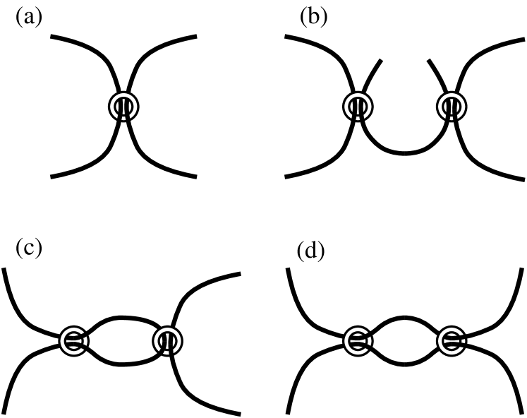
Figure 2: Schematic images for polymer chains paired by slip-links. Black curves and white circles represent polymer chains and slip-links, respectively. (a) two chains paired by a slip-link ($2(1,1)$), (b) three chains coupled by two slip-links ($3(1,1,2)$), and (c) and (d) two chains paired by two slip-links ($2(1,3)$ and $2(2,2)$).

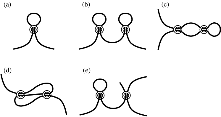
Figure 3: Schematic images for self-slip-linked polymer chains. Black curves and white circles represent polymer chains and slip-links, respectively. (a) a chain with an isolated loop ($1(2)$), (b) a chain with two isolated loops ($1(4)$), (c) a chain with nested (“8”-shaped) loops ($1(4^{\prime})$), (d) a chain with fused (“$\theta$”-shaped) loops ($1(4^{\prime\prime})$), and (e) paired two chains with an isolated loop ($2(3,1)$).

References

- 1 Doi, M.; Edwards, S. F. The Theory of Polymer Dynamics; Oxford University Press: Oxford, 1986
- 2 de Gennes, P. G. Scaling Concepts in Polymer Physics; Cornell University Press: Ithaca, New York, 1979
- 3 Matsen, M. W.; Bates, F. S. Macromolecules 1996, 29, 1091–1098
- 4 Matsen, M. W. J. Phys.: Cond. Mat. 2002, 14, R21–R47
- 5 Kawakatsu, T. Statistical Physics of Polymers: An Introduction; Springer Verlag: Berlin, 2004
- 6 Renner, C.; Löwen, H.; Barrat, J. L. Phys. Rev. E 1995, 52, 5091–5099
- 7 Obukhov, S.; Kobzev, D.; Perchak, D.; Rubinstein, M. J. Phys. I (France) 1997, 7, 563–568
- 8 van Ketel, W.; Das, C.; Frenkel, D. Phys. Rev. Lett. 2005, 94, 135703
- 9 Ball, R. C.; Doi, M.; Edwards, S. F.; Warner, M. Polymer 1981, 22, 1010–1018
- 10 Schieber, J. D. J. Chem. Phys. 2003, 118, 5162–5166
- 11 Hua, C. C.; Schieber, J. D. J. Chem. Phys. 1998, 109, 10018–10027
- 12 Masubuchi, Y.; Takimoto, J.; Koyama, K.; Ianniruberto, G.; Greco, F.; Marrucci, G. J. Chem. Phys. 2001, 115, 4387–4394
- 13 Doi, M.; Takimoto, J. Phil. Trans. R. Soc. Lond. A 2003, 361, 641–650
- 14 Nair, D. M.; Schieber, J. D. Macromolecules 2006, 39, 3386–3397
- 15 Rieger, J. Polym. Bull. 1987, 18, 343–346
- 16 Rieger, J. J. Phys. A: Math. Gen. 1988, 21, L1085–L1088
- 17 Rieger, J. J. Phys. A: Math. Gen. 1989, 22, 4540–4544
- 18 Sommer, J.-U. J. Chem. Phys. 1992, 97, 5777–5781
- 19 Metzler, R.; Hanke, A.; Dommersnes, P. G.; Kantor, Y.; Kardar, M. Phys. Rev. Lett. 2002, 88, 188101
- 20 Metzler, R.; Hanke, A.; Dommersnes, P. G.; Kantor, Y.; Kardar, M. Phys. Rev. E 2002, 65, 061103
- 21 Kardar, M. Eur. Phys. J. B 2008, 64, 519–523
- 22 Likhtman, A. E. Macromolecules 2005, 38, 6128–6139
- 23 Doi, M. Introduction to Polymer Physics; Clarendon Press: Oxford, 1996
- 24 Mayer, J. E.; Mayer, M. G. Statistical Mechanics; Wiley: New York, 1940
- 25 Yaoita, T.; Isaki, T.; Masubuchi, Y.; Watanabe, H.; Ianniruberto, G.; Greco, F.; Marrucci, G. J. Chem. Phys. 2008, 128, 154901
- 26 Masubuchi, Y.; Ianniruberto, G.; Greco, F.; Marrucci, G. J. Non-Newtonian Fluid Mech. 2008, 149, 87–92
- 27 Okuda, S.; Inoue, Y.; Masubuchi, Y.; Uneyama, T.; Hojo, M. submitted to Rheol. Acta.
- 28 James, H. M.; Guth, E. J. Chem. Phys. 1943, 11, 455–481
- 29 Deam, R. T.; Edwards, S. F. Phil. Trans. R. Soc. Lond. A 1976, 280, 317–353
- 30 Everaers, R. New J. Phys. 1999, 1, 12.1–12.54