The magnetic excitation spectra in BaFe₂As₂: a two-particle approach within DFT+DMFT

Abstract

We study the magnetic excitation spectra in the paramagnetic state of BaFe₂As₂ from the ab initio perspective. The one-particle excitation spectrum is determined within the combination of the density functional theory and the dynamical mean-field theory method. The two-particle response function is extracted from the local two-particle vertex function, also computed by the dynamical mean field theory, and the polarization function. This method reproduces all the experimentally observed features in inelastic neutron scattering (INS), and relates them to both the one particle excitations and the collective modes. The magnetic excitation dispersion is well accounted for by our theoretical calculation in the paramagnetic state without any broken symmetry, hence nematic order is not needed to explain the INS experimental data.

Neutron scattering experiments provide strong constraints on the theory of iron pnictides. Both the localized picture and the itinerant picture of the magnetic response have had some successes in accounting or even predicting aspects of the experiments. Calculations based on a spin model with frustrated exchange constants Goswami et al. (2010); Applegate et al. (2010) or with biquadratic interactions Wysocki et al. (2011) described well the neutron scattering experiments Diallo et al. (2009); Zhao et al. (2009). The itinerant magnetic model, based on an random phase approximation (RPA) form of the magnetic response, uses polarization functions extracted from density functional theory (DFT) Ke et al. (2011) or tight binding fits Park et al. (2010); Graser et al. (2010); Kaneshita and Tohyama (2010) and produces equally good descriptions of the experimental data.

Furthermore, DFT calculations predicted the stripe nature of the ordering pattern Dong et al. (2008) and the anisotropic values of the exchange constants which fit well the spin wave dispersion in the magnetic phase Han et al. (2009). The tight binding calculations based on DFT bands also predicted the existence of a resonance mode in the superconducting state Maier et al. (2009).

In spite of these successes, both itinerant and localized models require significant extensions to fully describe the experimental results. DFT fails to predict the observed ordered moment Han et al. (2009). Furthermore, adjusting parameters such as the arsenic height to reproduce the ordered moment, leads to a peak in the density of states at the Fermi level Ke et al. (2011), instead of the pseudogap, which is observed experimentally. The localized picture cannot describe the magnetic order in the FeTe material without introducing additional longer range exchange constants. Given that this material is more localized than the 122, the exchange constants would be expected to be shorter range. Furthermore, fits of the INS data require the use of anisotropic exchange constants well above the magnetic ordering temperature Harriger et al. (2010). However no clear phase transition to a nematic phase in this range has been detected.

In this Letter, we argue that the combination of density functional theory and dynamical mean field theory (DFT+DMFT) provides a natural way to improve both the localized and the itinerant picture, and connects the neutron response to structural material specific information and to the results of other spectroscopies.

Figure 1: (Color online) The Feynman diagrams for the Bethe-Salpeter equation. It relates the two-particle Green’s function ($\chi$) with the polarization ($\chi^{0}$) and the local irreducible vertex function ($\Gamma_{loc}^{irr}$). The non-local two-particle Green’s function is obtained by replacing the local propagator by the non-local propagator.

We compute the one-particle Green’s function using the charge self-consistent full potential DFT+DMFT method, as implemented in Ref. Haule et al. (2010), based on Wien2k code Blaha et al. (2001). We used the continuous-time quantum Monte Carlo (CTQMC) Haule (2007); Werner et al. (2006) as the quantum impurity solver, and the Coulomb interaction matrix as determined in Ref. Kutepov et al., 2010. The dynamical magnetic susceptibility $\chi(\textbf{q},\omega)$ is computed from the ab initio perspective by extracting the two-particle vertex functions of DFT+DMFT solution $\Gamma_{loc}^{irr}$ Jarrell (1992). The polarization bubble $\chi^{0}$ is computed from the fully interacting one particle Greens function. The full susceptibility is computed from $\chi^{0}$ and the two-particle irreducible vertex function $\Gamma_{loc}^{irr}$, which is assumed to be local in the same basis in which the DMFT self-energy is local, implemented here by the projector to the muffin-thin sphere Haule et al. (2010). In order to extract $\Gamma_{loc}^{irr}$, we employ the Bethe-Salpeter equation (see Fig. 1) which relates the local two-particle Green’s function ($\chi_{loc}$), sampled by CTQMC, with both the local polarization function ($\chi_{loc}^{0}$) and $\Gamma_{loc}^{irr}$:

$$\Gamma_{loc{\alpha_{1}\sigma_{1},\alpha_{2}\sigma_{2}\atop\alpha_{3}\sigma_{3},\alpha_{4}\sigma_{4}}}^{irr}(i\nu,i\nu^{\prime})_{i\omega}=\frac{1}{T}[(\chi_{loc}^{0})_{i\omega}^{-1}-\chi_{loc}^{-1}].$$ (1)

$\Gamma_{loc}^{irr}$ depends on three Matsubara frequencies ($i\nu$, $i\nu^{\prime}$; $i\omega$), and both the spin ($\sigma_{1-4}$) and the orbital ($\alpha_{1-4}$) indices, which run over $3d$ states on the iron atom. $T$ is the temperature.

Once the irreducible vertex $\Gamma_{loc}^{irr}$ is obtained, the momentum dependent two-particle Green’s function is constructed again using the Bethe-Salpeter equation (Fig. 1) by replacing the local polarization function $\chi_{loc}^{0}$ by the non-local one $\chi_{\textbf{q},i\omega}^{0}$:

$$\chi_{{\alpha_{1}\sigma_{1},\alpha_{2}\sigma_{2}\atop\alpha_{3}\sigma_{3},\alpha_{4}\sigma_{4}}}(i\nu,i\nu^{\prime})_{\textbf{q},i\omega}=[(\chi^{0})_{\textbf{q},i\omega}^{-1}-T\cdot\Gamma_{loc}^{irr}]^{-1}.$$ (2)

Finally, the dynamic magnetic susceptibility $\chi(\textbf{q},i\omega)$ is obtained by closing the two particle green’s function with the magnetic moment $\mu=\mu_{B}(\textbf{L}+2\textbf{S})$ vertex, and summing over frequencies ($i\nu$,$i\nu^{\prime}$), orbitals ($\alpha_{1-4}$), and spins ($\sigma_{1-4}$) on the four external legs

$$\chi(\textbf{q},i\omega)=T\sum_{i\nu,i\nu^{\prime}}\sum_{{\alpha_{1}\alpha_{2}\atop\alpha_{3}\alpha_{4}}}\sum_{{\sigma_{1}\sigma_{2}\atop\sigma_{3}\sigma_{4}}}\mu_{{\alpha_{1}\sigma_{1}\atop\alpha_{3}\sigma_{3}}}^{z}\mu_{{\alpha_{2}\sigma_{2}\atop\alpha_{4}\sigma_{4}}}^{z}\;\chi_{{\alpha_{1}\sigma_{1},\alpha_{2}\sigma_{2}\atop\alpha_{3}\sigma_{3},\alpha_{4}\sigma_{4}}}(i\nu,i\nu^{\prime})_{\textbf{q},i\omega}$$ (3)

The resulting dynamical magnetic susceptibility is obtained in Matsubara frequency ($i\omega$) space and it needs to be analytically continued to real frequencies ($\chi(\textbf{q},\omega)$). For the low frequency region, on which we concentrate here, the vertex $\Gamma_{loc}^{irr}$ is analytically continued by a quasiparticle-like approximation. We replace the frequency dependent vertex with a constant, i.e., $\Gamma_{loc{\alpha_{1}\sigma_{1},\alpha_{2}\sigma_{2}\atop\alpha_{3}\sigma_{3},\alpha_{4}\sigma_{4}}}^{irr}(i\nu,i\nu^{\prime})_{i\omega}\approx\bar{U}_{{\alpha_{1}\sigma_{1},\alpha_{2}\sigma_{2}\atop\alpha_{3}\sigma_{3},\alpha_{4}\sigma_{4}}}$, and require $\chi(q,i\omega=0)=\chi(q,\omega=0)$. This vertex $\bar{U}$ however retains important spin and orbital dependence.

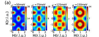
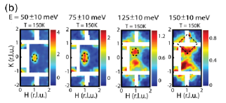
Figure 2: (Color online) (a) The constant energy plot of the theoretical dynamical structure factor, S($\textbf{q},\omega$) (=$\frac{\chi^{\prime\prime}(\textbf{q},\omega)}{1-e^{-\hbar\omega/k_{B}T}}$) at different energies (50meV, 75meV, 125meV, and 150meV) in the paramagnetic state (T=386 K) of BaFe₂As₂ as a function of momentum $\textbf{q}=$(H,K,L). L is here fixed at 1. (b) The corresponding inelastic neutron scattering data from Ref. Harriger et al., 2010.

Fig. 2(a) shows the calculated constant energy plot of the dynamical structure factor, S($\textbf{q},\omega$) in the paramagnetic state of BaFe₂As₂. Our theoretical results are calculated in the unfolded Brillouin zone of one Fe atom per unit cell, because magnetic excitations are concentrated primarily on Fe atoms, therefore folding, which occurs due to the two inequivalent arsenic atoms in the unit cell, is not noticeable in magnetic response Park et al. (2010). For comparison we also reproduce in Fig. 2(b) the INS experimental data from Ref. Harriger et al., 2010. At low energy (around $\omega$=50meV), the theoretical S($\textbf{q},\omega$) is strongly peaked at the ordering wave vector (H,K,L)=$(1,0,1)$ and it forms a clear elliptical shapes elongated in K direction. The elongation of the ellipse increases with energy ($\omega$=75meV) and around $\omega=$125meV the ellipse splits into two peaks, one peak centered at $(1,0.4,1)$ and the other at $(1,-0.4,1)$. At even higher energy ($\omega\approx$150meV) the magnetic spectra broadens and peaks from four equivalent wave vectors merge into a circular shape centered at wave vector $(1,1,1)$. At even higher energy (230meV, not shown in the figure) the spectra broadens further, and the peak becomes centered at the point $(1,1,1)$. These trends are all in good quantitative agreement with INS data from Fig. 2(b).

   

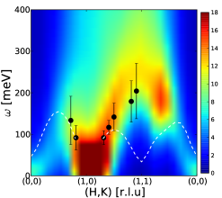
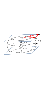
Figure 3: (Color online) S($\textbf{q},\omega$) along the special path in Brillouin zone marked by red arrow in the inset on the right. The inset shows the body-centered tetragonal (black line) and the unfolded (blue line) Brillouin zone. Black dots with error bars correspond to INS data from Ref. Harriger et al., 2010. The white dashed line shows the isotropic Heisenberg spin wave dispersion.

In Fig. 3, we display a contour plot of the theoretical S($\textbf{q},\omega$) as a function of frequency $\omega$ and momentum q along the special path in the unfolded Brillouin zone, sketched by a red line in the right figure. At low energies ($\omega<$80meV), S($\textbf{q},\omega$) is mostly concentrated in the region near the ordering vector $(1,0,1)$. Consistent with the elongation of the ellipse along the K direction in Fig. 2, the low energy ($\omega<$80meV) bright spot in Fig. 3 is extended further towards $(1,1,1)$ direction but quite abruptly decreases in the $(0,0,1)$ direction. The magnetic spectra in the two directions $(1,0,1)\rightarrow(0,0,1)$ and $(1,0,1)\rightarrow(1,1,1)$ are clearly different even at higher energy $\omega>100$meV. The peak position is moving to higher energy along both paths, but it fades away very quickly along the first path, such that the signal practically disappears at $(0.5,0,1)$. Along the second path $(1,0,1)\rightarrow(1,1,1)$, there remains a well defined excitation peak for which the energy is increasing, and at $(1,1,1)$ reaches the maximum value of $\approx 230$meV. Continuing the path from $(1,1,1)$ towards $(0,0,1)$ the peak energy decreases again and it fades away around $(0.5,0.5,1)$. The black dots display INS data with errors bars from Ref. Harriger et al., 2010. Notice a very good agreement between theory and experiment.

The white dashed line in Fig. 3 represents the spin wave dispersion obtained for the isotropic Heisenberg model using nearest neighbor $J_{1}$ and next nearest neighbor $J_{2}$ exchange constants and performing the best fit to INS data. This fit was performed in Ref. Harriger et al., 2010. The magnetic excitation spectra of an isotropic Heisenberg model show a local minimum at the wave vector $\textbf{q}=(1,1,1)$, which is inconsistent with our theory and with the experiment. To better fit the experimental data with a Heisenberg-like model, very anisotropic exchange constants need to be assumed Harriger et al. (2010), which raised speculations about possible existence of nematic phase well above the structural transition of BaFe₂As₂. Since the DFT+DMFT results can account for all the features of the measured magnetic spectra without invoking any rotationally symmetry breaking the presence of nematicity in the paramagnetic tetragonal state at high temperature is unlikely.

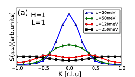
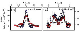
Figure 4: (Color online) (a) The wave vector K dependence (H=1,L=1) of S($\textbf{q},\omega$) at several frequencies. (b) The corresponding INS data at $\omega$=19meV and (c) 128meV reproduced from Ref. Harriger et al., 2010. The red circles correspond to the paramagnetic state at $T$=150K and the blue diamonds to the magnetic state at $T$=7K.

In Fig. 4(a) we show constant frequency cuts in the K direction (from $(1,-1,1)$ through $(1,0,0)$ to $(1,1,1)$) of S($\textbf{q},\omega$) displayed in Fig. 3. For comparison we also show the corresponding INS measurements from Ref. Harriger et al., 2010 as red circles in Fig. 4(b) and (c). At $\omega$=20meV, the spectrum has a sharp peak centered at the ordering vector $(1,0,1)$. At $\omega$=50meV, the spectrum still displays a peak at $(1,0,1)$ but the intensity is significantly reduced. With increasing frequency $\omega$, the peak position in S($\textbf{q},\omega$) moves in the direction of $(1,1,1)$, and at 128meV peaks around $(1,0.4,1)$. The shift of the peak is accompanied with substantial reduction of intensity at ordering wave vector $(1,0,1)$. At even higher energy of 250meV only a very weak peak remains, and it is centered at the wave vector $(1,1,1)$. The position of peaks as well as their frequency dependence is in very good agreement with INS experiments of Ref. Harriger et al., 2010 displayed in Fig. 4(b) and (c).

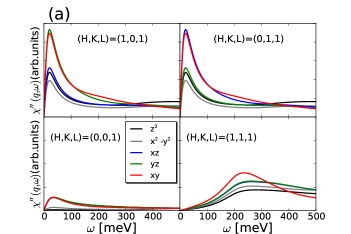
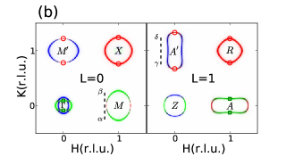
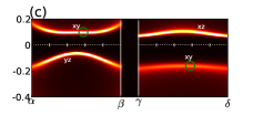
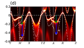
Figure 5: (Color online) (a) The Fe $d$ orbital resolved dynamical magnetic susceptibility at $T$=386K for distinct wave vectors q=$(1,0,1)$, $(0,1,1)$, $(0,0,1)$, and $(1,1,1)$. Different colors correspond to different orbital contributions. (b) The Fermi surface in the $\Gamma$ and $Z$ plane at $T$=73K colored by the orbital characters: $d_{xz}$(blue), $d_{yz}$(green), and $d_{xy}$(red). The small symbols mark the regions in the Fermi surface, where nesting for the wave vector q=$(1,0,1)$ is good. (c) The zoom-in of $A(\textbf{k},\omega)$ along the path marked by black dashed line in Fig. 5(b). The green open circles indicate the two relevant bands of $d_{xy}$ character which give rise to the peak in magnetic excitation spectra near 230meV at q=$(1,1,1)$. (d) $A(\textbf{k},\omega)$ computed in one Fe atom per unit cell at $T$=73K. The green arrows mark the same bands which give rise to 230meV peak. The DFT bands are overlayed by white dashed lines. The blue arrows mark corresponding DFT bands of $d_{xy}$ character.

Fig. 5(a) resolves the dynamical magnetic susceptibility $\chi$ of Eq. 3 in the orbital space $\chi_{\alpha}=T\sum_{i\nu,i\nu^{\prime}}\sum_{\beta}\sum_{{\sigma_{1}\sigma_{2}\atop\sigma_{3}\sigma_{4}}}\mu_{\sigma_{1}\sigma_{3}}^{z}\mu_{\sigma_{2}\sigma_{4}}^{z}\;\chi_{{\alpha\sigma_{1},\beta\sigma_{2}\atop\alpha\sigma_{3},\beta\sigma_{4}}}(i\nu,i\nu^{\prime})$ such that $\chi=\sum_{\alpha}\chi_{\alpha}$. At the magnetic ordering vector q=$(1,0,1)$, $\chi_{\alpha}^{\prime\prime}$ increases sharply with frequency near $\omega=0$ for all orbitals and is strongly suppressed above 100meV reaching the maximum around 20meV. At this wave vector, the dominant contributions at low energy come from the $d_{xy}$ and the $d_{yz}$ orbitals. The magnetic susceptibility at q=$(0,1,1)$ in Fig. 5(a) shows the same trend as orbitally resolved spectra at q=$(1,0,1)$, except that $d_{xz}$ and $d_{yz}$ switch their roles due to the $C_{4}$ symmetry of the Fe square lattice.

These dominant orbital contributions to $\chi$ are also reasonably captured in the polarization bubble $\chi^{0}$ (not shown here), hence these excitations could be understood in terms of the Fermi surface nesting. The orbital resolved Fermi surface is displayed in Fig. 5(b) at both the $\Gamma$-plane and the $Z$-plane. Most of the weight in $\chi^{0}$ comes from the diagonal terms, i.e., $\chi^{0}_{\alpha,\alpha}$, hence the Fermi surfaces with the same color in Fig. 5(b) but separated by the wave vector $(1,0,1)$ give dominant contribution. The intra-orbital $d_{yz}$ low energy spectra comes mostly from the transitions between the green parts of the hole pocket at $\Gamma$ and the green parts of the electron pocket at $A$, marked with green squares ($\square$) in Fig. 5(b). Since the electron pocket at $A$ is elongated in H direction, the nesting condition occurs mostly in the perpendicular K direction, hence the elliptical excitations at low energy in Fig. 2 are elongated in K but not in H direction. The intra-orbital $d_{xy}$ transitions are pronounced between the electron pocket at $M^{\prime}$ and the hole pocket at $R$, as well as between the electron pocket at $A^{\prime}$ and the hole pocket at $X$ (marked with red $\bigcirc$). This large spin response at $(1,0,1)$ gives rise to the low energy peak in Fig. 3.

We note that the particle-hole response, encoded in polarization bubble $\chi^{0}$, is especially large when nesting occurs between an electron pockets and a hole pocket, because the nesting condition extends to the finite frequency, and is not cut-off by the Fermi functions.

The low energy magnetic excitations at wave vectors $\textbf{q}=(0,0,1)$ and $\textbf{q}=(1,1,1)$ can come only from electron-electron or hole-hole transitions, hence both responses are quite small, as seen in Fig. 5(a). While the magnetic response at $\textbf{q}=(0,0,1)$ is small but finite, the spin response at $\textbf{q}=(1,1,1)$ is almost gapped. This is because the hole-hole transitions from $\Gamma$ to $R$ or electron-electron transitions from $M$ to $A^{\prime}$ do not involve any intra-orbital transitions, and hence are even smaller than transitions at the wave vector $(0,0,1)$.

At finite energy transfer, the spin excitations come from electronic states away from the Fermi energy, and can not be easily identified in the Fermi surface plot. Hence it is more intriguing to find the dominant contribution to the peak at $\omega\approx 230$meV and $\textbf{q}=(1,1,1)$. This peak gives rise to the 230meV excitations at $(1,1,1)$ in Fig. 3. A large contribution to this finite frequency excitation comes from a region near the two electron pockets at $M$ and $A^{\prime}$ marked with black dashed line in Fig. 5(b). We display in Fig. 5(c) the one electron spectral function across these dashed lines in the Brillouin zone to show an important particle hole transition from the electrons above Fermi level at the $M$ point and the flat band at -200meV around the $A^{\prime}$ point, both of $d_{xy}$ character. We note that due to large off diagonal terms in the two particle vertex $\Gamma$, all orbital contributions to $\chi$ develop a peak at the same energy, although only $d_{xy}$ orbital displays a pronounced peak in $\chi^{0}$.

Fig. 5(d) displays the one electron spectral function in a path through the Brillouin zone, corresponding to one Fe atom per unit cell. Within DFT+DMFT the quasi-particle bands are renormalized by a factor of 2-3 compared to the corresponding DFT bands (white dashed lines). The green arrow marks the $d_{xy}$ band which contributes to the peak in $S(\textbf{q},\omega)$ near 230meV and $\textbf{q}=(1,1,1)$. In DFT calculation, this $d_{xy}$ intra-orbital transition is also present, but occurs at much higher energy of the order of 400-600meV, marked by blue arrows. The over-estimation of the peak energy at q=$(1,1,1)$ was reported in LSDA calculation of Ref. Ke et al., 2011.

In this Letter, we have extended the DFT+DMFT methodology to compute the two particle responses in a realistic multi-orbital DFT+DMFT setting. With the same parameters which were used to successfully describe the optical spectra and the magnetic moments of this material Yin et al. (2011), we obtained a coherent description of the experimental neutron scattering results. Our theory ties the magnetic response to the fermioloy of the model, and quantifies the departure from both purely itinerant and localized pictures.

Acknowlegements: We are grateful to Pencheng Dai for discussions of his experimental results. This research was supported in part by the National Science Foundation through TeraGrid resources provided by Ranger (TACC) under grant number TG-DMR100048.

References

- Goswami et al. (2010) P. Goswami, R. Yu, Q. Si, and E. Abrahams, arXiv:1009.1111 (2010).
- Applegate et al. (2010) R. Applegate, J. Oitmaa, and R. R. P. Singh, Phys. Rev. B 81, 024505 (2010).
- Wysocki et al. (2011) A. L. Wysocki, K. D. Belashchenko, and V. P. Antropov, doi:10.1038/nphys1933 (2011).
- Diallo et al. (2009) S. O. Diallo, V. P. Antropov, T. G. Perring, C. Broholm, et al., Phys. Rev. Lett. 102, 187206 (2009).
- Zhao et al. (2009) J. Zhao, D. T. Adroja, D.-X. Yao, R. Bewley, et al., Nature Physics 5, 555 (2009).
- Ke et al. (2011) L. Ke, M. van Schilfgaarde, J. Pulikkotil, T. Kotani, and V. Antropov, Phys. Rev. B 83, 060404 (2011).
- Park et al. (2010) J. T. Park, D. S. Inosov, A. Yaresko, S. Graser, et al., Phys. Rev. B 82, 134503 (2010).
- Graser et al. (2010) S. Graser, A. F. Kemper, T. A. Maier, H.-P. Cheng, et al., Phys. Rev. B 81, 214503 (2010).
- Kaneshita and Tohyama (2010) E. Kaneshita and T. Tohyama, Phys. Rev. B 82, 094441 (2010).
- Dong et al. (2008) J. Dong, H. J. Zhang, G. Xu, Z. Li, et al., Europhys. Lett. 83, 27006 (2008).
- Han et al. (2009) M. J. Han, Q. Yin, W. E. Pickett, and S. Y. Savrasov, Phys. Rev. Lett. 102, 107003 (2009).
- Maier et al. (2009) T. A. Maier, S. Graser, D. J. Scalapino, and P. Hirschfeld, Phys. Rev. B 79, 134520 (2009).
- Harriger et al. (2010) L. W. Harriger, H. Luo, M. Liu, T. G. Perring, et al., arXiv:1011.3771 (2010).
- Haule et al. (2010) K. Haule, C.-H. Yee, and K. Kim, Phys. Rev. B 81, 195107 (2010).
- Blaha et al. (2001) P. Blaha, K. Schwarz, G. K. H. Madsen, K. Kvasnicka, et al., Wien2K (Karlheinz Schwarz, Technische Universitat Wien, Austria, 2001).
- Haule (2007) K. Haule, Phys. Rev. B 75, 155113 (2007).
- Werner et al. (2006) P. Werner, A. Comanac, L. de’ Medici, M. Troyer, and A. J. Millis, Phys. Rev. Lett. 97, 076405 (2006).
- Kutepov et al. (2010) A. Kutepov, K. Haule, S. Y. Savrasov, and G. Kotliar, Phys. Rev. B 82, 045105 (2010).
- Jarrell (1992) M. Jarrell, Phys. Rev. Lett. 69, 168 (1992).
- Yin et al. (2011) Z. P. Yin, K. Haule, and G. Kotliar, Nature Physics 7, 294 (2011).