An improved, “phase-relaxed” ${\mathcal{F}}$-statistic for gravitational-wave data analysis

Abstract

Rapidly rotating, slightly non-axisymmetric neutron stars emit nearly periodic gravitational waves (GWs), quite possibly at levels detectable by ground-based GW interferometers. We refer to these sources as “GW pulsars”. For any given sky position and frequency evolution, the ${\mathcal{F}}$-statistic is the optimal (frequentist) statistic for the detection of GW pulsars. However, in an ”all-sky” searches for previously unknown GW pulsars, it would be computationally intractable to calculate the (fully coherent) ${\mathcal{F}}$-statistic at every point of (suitably fine) grid covering the parameter space: the number of gridpoints is many orders of magnitude too large for that. Therefore, in practice some non-optimal detection statistic is used for all-sky searches. Here we introduce a “phase-relaxed” ${\mathcal{F}_{pr}}$-statistic, which we denote ${\mathcal{F}_{pr}}$, for incoherently combining the results of fully coherent searches over short time intervals. We estimate (very roughly) that for realistic searches, our ${\mathcal{F}_{pr}}$ is $\sim 10-15\%$ more sensitive than the “semi-coherent” ${\mathcal{F}}$-statistic that is currently used. Moreover, as a byproduct of computing ${\mathcal{F}_{pr}}$, one obtains a rough determination of the time-evolving phase offset between one’s template and the true signal imbedded in the detector noise. Almost all the ingredients that go into calculating ${\mathcal{F}_{pr}}$ are already implemented in the LIGO Algorithm Library, so we expect that relatively little additional effort would be required to develop a search code that uses ${\mathcal{F}_{pr}}$.

I Introduction

The ${\mathcal{F}}$-statistic is the optimal frequentist statistic for the detection of nearly monochromatic gravitational waves (GWs) from a neutron star with known (or assumed) sky location and frequency evolution jks . The basic idea behind the ${\mathcal{F}}$-statistic is simply this: for any given sky location and frequency evolution, the set of possible GW signals forms a four-dimensional (real) vector space cf94 ; jks . The four basis vectors are the two quadratures ($\rm sin$ and $\rm cos$) of each of the two polarization bases, $+$ and $\times$. Because the set is a vector space (not just a 4-d manifold), it is computationally trivial to maximize the likelihood function over this set; ${\mathcal{F}}$ is the maximized log-likelihood. For Gaussian noise, the probability distribution function (pdf) of ${\mathcal{F}}$ is also particularly simple: a (perhaps non-central) $\chi^{2}$ distribution with $4$ degrees of freedom. In their original paper by Jaranowski, Krolak & Schutz jks (hereinafter referred to JKS), the ${\mathcal{F}}$-statistic was derived only for the case of a single GW detector and a single GW pulsar. Cutler & Schutz CutlerSchutz2005 showed how the ${\mathcal{F}}$-statistic can be generalized in a straightforward manner to the cases of 1) a network of detectors noise curves, and 2) an entire collection of known sources.

In practice, searches for nearly-monochromatic GWs are separated into a few different types, depending on how much is know about the source. The different types of searches can have vastly different computational requirements. While the search for a GW counterpart to a known radio pulsar is trivial in terms of computational burden, “all-sky” searches for GW pulsars with no known counterpart (and hence unknown frequency and frequency derivatives) are currently limited by the available computational power. That is, we could dig deeper into the existing data sets if we possessed either larger computational resources or more efficient algorithms. In this paper we demonstrate a way of significantly improving on the existing algorithms.

Currently, the most sensitive all-sky searches are based on the following idea EH . For a GW pulsar with unknown frequency evolution (i.e., unknown $f$, $\dot{f}$, etc.), computational power required for an optimal (i.e, fully coherent, ${\mathcal{F}}$-based) search grows as a high-power of the total observation time, $T$. Therefore in practice one divides $T$ into some number N (typically of order $10^{2})$ short intervals of duration $\Delta T=T/N$, performs an optimal, coherent search one each short interval, and then “adds up” the power from the all subintervals. More specifically, the current method is to calculate a “semi-coherent” detection statistic ${\mathcal{F}}_{sc}$, defined as the sum of the ${\mathcal{F}}$ values from each of the short intervals:

$${\mathcal{F}_{sc}}\equiv\sum_{i=1}^{N}{\mathcal{F}}_{i}\,.$$ (1)

Because calcuting each ${\mathcal{F}}_{i}$ involves a maximization over $4$ free parameters, the pdf for ${2\mathcal{F}_{sc}}$ is a $\chi^{2}$ distribution with $4N$ d.o.f. But this is far more parameters than are actually needed to describe the physical system! Consider the very first interval. The imbedded GW signal is described by $4$ parameters: $(h_{0},\iota,\psi,\Phi)$. But the triplet $(h_{0},\iota,\psi)$ are the same for all $N$ intervals. All that changes from interval to interval is the overall phase $\Phi$. Assuming maximum ignorance of the signal’s phase evolution, one therefore needs $N-1$ additional phases to fully describe the signal. So the GW signal is fully described by only $N+3$ parameters. We define ${\mathcal{F}_{pr}}$ to be the maximized log-likelihood on this $N+3$-dimensional space. Our main aims in this paper are (i) to demonstrate an efficient algorithm for calculating ${\mathcal{F}_{pr}}$ and (ii) to and to illustrate its superiority as a detection statistic (superior in the sense of improved ROC curves, where ROC stands for ”Receiver Operating Characteristics”).

We note that our work is rather similar in spirtit to a recent paper by Dergachev Dergachev2010 , though we believe that we have advanced the idea considerably further. We note, too, a recent paper by Pletsch pletsch2011 , which addresses the followng, rather different weakness in the detection statistic Eq. (1). To understand the problem, let $(t_{0},t_{1},\cdots,t_{N})$ be the boundary points of the $N$ short intervals, and consider any one such boundary time, say $t_{50}$. In Eq. (1), data sampled ony slightly earlier than $t_{50}$ gets combined incoherently with data sampled only slightly later than $t_{50}$, which clearly exacts a price in sensitivity. Pletsch overcomes this problem (which stems from the rather arbitrary choice of boundary points) using his “sliding window” technique pletsch2011 . We suspect that relatively simple refinements of the detection statistic that we develop in this paper could also capitalize on Pletsch’s basic insight, but we leave such refinements to future work.

The plan of this paper is as follows. In Sec. II we briefly review the fully coherent ${\mathcal{F}}$-statistic, partly to establish notation. We generally try to align our notation with that of JKS, to ease comparison with their work. We also review the (currently used) semi-coherent ${\mathcal{F}}$-statistic and its properties.

As further motivation for our work, in Sec. IV we consider a “warm-up” problem that we can easily treat analytically and that qualitatively has much in common with our actual problem. In Sec. V, in order to illustrate both the use of ${\mathcal{F}_{pr}}$, we present numerical results for one example search. For the same search, we also investigate the relative power/sensitivty of ${\mathcal{F}_{pr}}$ versus ${\mathcal{F}_{sc}}$. Our conclusions are summarized in Sec. VI.

This paper represents our ”first-cut” analysis of the ${\mathcal{F}_{pr}}$ statistic. There remains significant follow-up work to better elucidate the properties of ${\mathcal{F}_{pr}}$ and to implement it in realistic, hierarchical searches. This future work is also summarized in Sec. VI.

II Review of Signal Processing for GW pulsars

In this section we review the rudiments of signal processing that we will require, partly to fix notation. We also review both the coherent and semi-coherent versions of the ${\mathcal{F}}$-statistic. For simplicity of exposition, in this paper we will restrict the case of a single detector, and assume that the detector noise is stationary. The extension to the more realistic case of multiple detectors with slowly changing noise spectra is completely straightforward.

II.1 Mathematics of signal processing

We begin by reviewing the basic mathematics of signal processing. For more details, we refer the reader to Thorne (1987), Finn & Chernoff (1993), and/or Cutler & Flanagan (1994) 300years ; finn2 ; cf94 .

Assuming that the noise is stationary and Gassuian, the noise spectral density $S_{h}(f)$ determines a natural inner product $\left(\ldots|\ldots\right)$ on the vector space of all detector outputs $x(t)$:

$$\left({\bf x}\,|\,{\bf y}\right)\equiv 2\,\int_{-\infty}^{\infty}df\,\,\frac{\tilde{x}^{*}(f)\tilde{y}(f)}{S_{h}(f)}\,,$$ (2)

where $\tilde{x}(f)$ and $\tilde{y}(f)$ denote the Fourier transforms of $x(t)$ and $y(t)$, and $S_{h}(f)$ is the single-sided spectral density of the noise. In terms of this inner product, the probability distribution function (pdf) for the noise ${\bf n}(t)$ takes the form

$${\rm pdf}[{\bf n}]\,=\,{\cal N}e^{-\left({\bf n}|{\bf n}\right)/2},$$ (3)

where $\cal N$ is a normalization constant. Using $\big{<}\cdots\big{>}$ to denote ”expectation value” (over many realizations of the noise), it follows from Eq. (3) that

$$\big{<}\,\left({\bf x}\,|\,{\bf n}\right)\left({\bf y}\,|\,{\bf n}\right)\,\big{>}=\left({\bf x}\,|\,{\bf y}\right)\,.$$ (4)

In this paper, we will be concerned with waveforms $h(t)$ that are nearly monochromatic (here meaning that their frequencies $f(t)$ are slowly varying). In this case their inner product is equally simple in the time domain. Taking the measurement time interval to be $0$ to $T$, we have

$$\left({\bf h_{1}}\,|\,{\bf h_{2}}\right)=2\,\int_{0}^{T}\,\,\frac{{\tilde{h}_{1}}(t){\tilde{h}_{2}}(t)}{S_{h}\big{(}f(t)\big{)}}\,dt\,,$$ (5)

II.2 The fully coherent ${\mathcal{F}}$-statistic

Next we briefly review the use of the coherent F-statistic in GW pulsar searches. For more details we refer the reader to Cutler & Schutz (2005) CutlerSchutz2005 . Consider a nearly monochromatic GW signal from an individual source with known sky location and known frequency evolution $f(t)$. The GW signal is then characterized by four remaining unknowns: an overall amplitude $A$ (equivalent to the combination $h_{0}\ {\rm sin}\ \zeta\,{\rm sin}^{2}\theta$ in the notation of JKS), two angles $\iota$ and $\psi$ that characterize the waves’ polarization (equivalent to determining the direction of the NS’s spin axis), and an overall phase $\Phi$.

The GW signal $h(t)$ registered by the detectgor depends nonlinearly on $\iota,\psi,\Phi$, but, crucially, one can make a simple change of variables–to $\big{(}\lambda^{1},\lambda^{2},\lambda^{3},\lambda^{4}\big{)}$–such that dependence of $h(t)$ is linear in these new variables:

$$h(t)=\sum_{a=1}^{4}\lambda^{a}h_{a}(t)$$ (6)

where the four basis waveforms $h_{a}^{\alpha}(t)$ are defined by

$$h_{1}(t)=F_{+}(t)\rm cos\Phi(t),\ h_{2}(t)=F_{\times}(t)\rm cos\Phi(t),\ \ \ \ \ \ \ \ \$$

$$h_{3}(t)=F_{+}(t)\rm sin\Phi(t),\ h_{4}(t)=F_{\times}(t)\rm sin\Phi(t)\,.\ \ \ \ \ \ \ \ \$$ (7)

Here $\Phi(t)$ is the waveform phase at the detector:

$$\Phi(t)\approx 2\pi\int^{t}f(t^{\prime})dt^{\prime}\,,$$ (8)

where $f(t^{\prime})$ is the measured GW frequency at the detector at time $t^{\prime}$. The measured frequency includes the Doppler effect from the detector’s motion relative to the source, as well as Einstein and Shapiro delays associated with the Earth’s orbit around the Sun. When the GW pulsar is in a binary, then $f(t^{\prime})$ also includes the Roemer, Einstein, and Shapiro delays associated with that binary orbit. ( We emphasize that the known-pulsar searches described here do not require that the GW pulsar be isolated, but just that there exists an accurate timing model for the emitted waves.) The $F_{+}(t)$ and $F_{\times}(t)$ terms in Eq. (II.2) are the beam-pattern functions describe the detector’s response to the $+$ and $\times$ polarizations, respectively. We note that the exact form of $F_{+}(t)$ and $F_{\times}(t)$ depends on one’s convention for decomposing the waveform into “plus” and “cross” polarizations; a one-parameter family of choices is possible, corresponding to the freedom to rotate the axes around the line of sight. JKS follow the conventions of Bonazzola & Gourgoulhon Bonazzola .

Next we define the $4\times 4$ matrix $\Gamma_{ab}$ by

$$\Gamma_{ab}\equiv\big{(}\frac{\partial{\bf h}}{\partial\lambda^{a}}\,|\,\frac{\partial{\bf h}}{\partial\lambda^{b}}\big{)}=\big{(}{\bf h_{a}}\,|\,{\bf h_{b}}\big{)}\,.$$ (9)

Because both the observation time and $1$ day (the timescale on which the $F_{+,{\times}}^{\alpha}(t)$ vary) are vastly larger than the period of the sought-for GWs (typically $10^{-2}-10^{-3}$ s), we can replace $\rm cos^{2}\Phi(t)$, $\rm sin^{2}\Phi(t)$, and $\rm cos\Phi(t)\rm sin\Phi(t)$ by their time-averages: $\rm cos^{2}\Phi(t),\rm sin^{2}\Phi(t)\rightarrow\frac{1}{2}$, while $\rm cos\Phi(t)\rm sin\Phi(t)\rightarrow 0$. Then we have

$$\Gamma_{11} \approx \int{F_{+}(t)\ F_{+}(t)S_{h}^{-1}\big{(}f(t)\big{)}\,dt}$$

$$\Gamma_{12} \approx \int{F_{+}(t)\ F_{\times}(t)S_{h}^{-1}\big{(}f(t)\big{)}\,dt}$$

$$\Gamma_{22} \approx \int{F_{\times}(t)F_{\times}(t)S_{h}^{-1}\big{(}f(t)\big{)}\,dt}\,;$$ (10)

additionally, $\Gamma_{33}\approx\Gamma_{11}$, $\Gamma_{34}\approx\Gamma_{12}$, $\Gamma_{44}\approx\Gamma_{22}$, and $\Gamma_{13}\approx\Gamma_{14}\approx\Gamma_{23}\approx\Gamma_{24}\approx 0$.

The best-fit values of $\lambda^{a}$ satisfy

$${\frac{\partial}{\partial\lambda^{a}}}({\bf x}-\sum_{b}\lambda^{b}{\bf h_{b}}\,|\,x-\sum_{c}\lambda^{c}{\bf h_{c}})=0$$ (11)

implying

$$\lambda^{a}=\sum_{b}\,(\Gamma^{-1})^{ab}({\bf x}\,|\,{\bf{h_{b}}})\,.$$ (12)

Then $2{\mathcal{F}}$, which is defined to be twice the log of the maximized likelihood ratio, is just

$$2{\mathcal{F}} = ({\bf x}|{\bf x})-({\bf x}-\sum_{b}\lambda^{b}{\bf h_{b}}\ \,|\,\ {\bf x}-\sum_{c}\lambda^{c}{\bf h_{c}})$$ (13)

$$= \sum_{a,d}\,(\Gamma^{-1})^{ad}({\bf x}|{\bf h_{a}})({\bf x}|{\bf h_{d}})\,.$$

Using $2{\mathcal{F}}$ as one’s detection statistic satisfies the Neyman-Pearson criterion for an optimum test: it minimizes the false dismissal (FD) probability for any given false alarm (FA) probability.

Writing ${\bf x}={\bf n}+{\bf h}$, and plugging into Eq. (13), we find

$$\big{<}2{\mathcal{F}}\big{>}=4+({\bf h}\ |\ {\bf h})\,,$$ (14)

where we have used Eq. (4) and the fact that $\big{<}({\bf h}\ |\ {\bf n})\big{>}\ =\ 0$. More generally, it is easy to show that $y\equiv 2{\mathcal{F}}$ follows a $\chi^{2}$ distribution with $4$ degrees of freedom (d.o.f) and non-centrality parameter $\rho^{2}\equiv({\bf h}|{\bf h})$:

$$P(y)=\chi^{2}(y|4;\rho^{2})\,.$$ (15)

As pointed out by JKS, if we use the following complexified variables,

$$2F_{a}\equiv({\bf x}|{\bf h_{1}}-i{\bf h_{3}})\ ,\ \ 2F_{b}\equiv({\bf x}|{\bf h_{2}}-i{\bf h_{4}})\ ,$$ (16)

then the expression (13) for $2{\mathcal{F}}$ can be re-written in a particularly simple form: Eq. (13) becomes

$$2{\mathcal{F}}=\frac{8}{D}\big{[}\negthinspace B|F_{a}|^{2}+A|F_{b}|^{2}-2C\Re(F_{a}F^{*}_{b})\big{]}\,.$$ (17)

where

$$A\equiv\,({\bf h_{1}}|{\bf h_{1}})\,,\ \ \ B\equiv({\bf h_{2}}|{\bf h_{2}})\,,\ \ \ C\equiv({\bf h_{1}}|{\bf h_{2}})\,,$$ (18)

and $D\equiv AB-C^{2}$. (Note that the A,B,C terms defined here are, in the single-detector case, larger than the A,B,C terms in JKS by a factor of the observation time $T$.)

II.3 The “semi-coherent” ${\mathcal{F}}$-statistic

As mentioned above, the current method of incoherently combining the coherent results from successive intervals is just to sum of the ${\mathcal{F}}$-statistics from all the intervals:

$$2{\mathcal{F}_{sc}}\equiv\sum_{i=1}^{N}2{\mathcal{F}_{i}}\,.$$ (19)

It also easy to show that $y\equiv 2{\mathcal{F}_{sc}}$ follows a $\chi^{2}$ distribution with $4N$ degrees of freedom:

$$P(y)=\chi^{2}(y|4N;\rho^{2})\,.$$ (20)

where the non-centrality parameter $\rho^{2}=\sum_{i=1}^{N}\rho^{2}_{i}$.

In the cases of interest to us, $4N$ will generally be large, and then the $\chi^{2}$ distribution with $4N$ d.o.f. can often be approximated as a Gaussian. Let $y\equiv 2{\mathcal{F}}$, and let $\rho_{tot}^{2}\equiv\sum_{i=1}^{N}\rho_{i}^{2}$. Then

$$P(y)=\chi^{2}(y|4N;\rho_{tot}^{2})\approx(8\pi\,N)^{-1/2}e^{-(y-<y>)^{2}/(8N)}$$ (21)

where $<y>=4N+\rho_{tot}^{2}$. For example, using this approximation (and the fact that for a Gaussian $P(y)$, events $2.326\sigma$ above the mean occur $1\%$ of the time), we see that the threshhold value $y_{th}$ that yields a $1\%$ FA probability is

$$y_{th}\approx 4N+2.326\sqrt{8N}\ \ {\rm(large\,N)}\,.$$ (22)

III The “phase-relaxed” ${\mathcal{F}}$-statistic

We are now ready to define ${\mathcal{F}_{pr}}$. Basically, ${\mathcal{F}_{pr}}$ coincides with the full matched-filtering $SNR^{2}$, under the assumption that the manifold of waveforms is $N+3$-dimensional (i.e., 4 parameters for the first segment, and $N-1$ for the relative phase offsets of the remaining segments). What makes ${\mathcal{F}_{pr}}$ useful in practice is that we have also found a simple and efficient method for calculating it.

III.1 Motivation and definition

We begin by defining complex basis functions $H_{+}$ and $H_{\times}$ by

$$H_{+}\equiv h_{1}-ih_{3}\ \ \ \ ,\ \ \ H_{\times}\equiv h_{2}-ih_{4}\,.$$ (23)

This complex representation is especially convenient for our purposes because $H_{+}$ and $H_{\times}$ both transform very simply under an overall phase shift in $\Phi(t)$: under $\Phi(t)\rightarrow\Phi(t)+\delta$, $H_{+}$ and $H_{\times}$ transform as $H_{+}(t)\rightarrow e^{-i\delta}H_{+}(t)$ and $H_{\times}(t)\rightarrow e^{-i\delta}H_{\times}(t)$. (Note that the minus sign in the exponent in the term $e^{-i\delta}$ stems from the minus signs in the definitions of of $H_{+}$ and $H_{\times}$ in Eq.( 23). For these complexified signals, our usual inner product becomes a Hermitian one; for nearly monochromatic signals near frequency $f$, this Hermitian inner product is given simply by

$$\big{(}{\bf x}\,|\,{\bf y}\big{)}=\frac{2}{S_{h}(f)}\int{x^{*}(t)y(t)dt}\ \ \,.$$ (24)

Clearly $\big{(}{\bf x}\,|\,{\bf y}\big{)}=\big{(}{\bf y}\,|\,{\bf x}\big{)}^{*}$.

Next we define $\Gamma_{\alpha\beta}$ by

$$\Gamma_{\alpha\beta}\equiv\big{(}H_{\alpha}\,|\,H_{\beta}\big{)}=\Gamma^{*}_{\beta\alpha}\,,$$ (25)

where $\alpha$ and $\beta$ run over $+,\times$. It follows immediately that for GW data $x(t)$, (twice the) ${\mathcal{F}}$-statistic is given by

$$2{\mathcal{F}}=\big{(}\Gamma^{-1}\big{)}^{\alpha\beta}\big{(}H_{\alpha}\,|\,{\bf x}\big{)}\big{(}{\bf x}\,|\,H_{\beta}\big{)}\,.$$ (26)

Now imagine breaking up the full integration time $T$ into N intervals of duration $\Delta T_{i}$, for $i=1,2,\cdots,N$. (We expect that in practice the $\Delta T_{i}$ will generally be of approximately the same length, but this is not required.) Next define $x^{i}(t)$ to be the restriction of $x(t)$ to the $i^{th}$ interval; i.e, $x^{i}(t)=x(t)$ for $t$ in the $i^{th}$ interval, and $x^{i}(t)=0$ for $t$ outside the $i^{th}$ interval. Then clearly we have

$$2{\mathcal{F}}=\big{(}\Gamma^{-1}\big{)}^{\alpha\beta}\bigg{(}\sum_{i}\big{(}H_{\alpha}\,|\,{\ \bf x^{i}}\big{)}\big{(}\sum_{j}\big{(}{\bf x^{j}}\,|\,H_{\beta}\big{)}\bigg{)}\,.$$ (27)

To motivate our definition of ${\mathcal{F}}_{pr}$, recall that if we had practically limitless computer power at our disposal, then the most sensitive search would be a coherent matched-filter search over a fine grid covering the entire GW-pulsar parameter space. However for “blind” GW pulsar searches (i.e., searches for GW pulsars whose sky location and/or time-changing frequency are unknown), maintaining phase coherence between the template signal and true imbedded signal, over timescales of months to years, would require an extremely fine grid on parameter space, and (one easily shows) many of orders of magnitude more computing power than is realistic BCCS

The basic idea behind “semi-coherent” searches is to employ a detection statistic that is less sensitive to phase decoherence across the whole observation time, which allows one to use a much coarser grid on parameter space. In effect, one sacrifices some sensitivity in the interest of computational practicality. For our phase-relaxed ${\mathcal{F}}$-statistic, the idea is that the search-template signal should remain approximately in phase with the true, imbedded signal in each interval $\Delta T_{i}$–up to some constant phase “offset $\delta_{i}$–but that the $\delta_{i}$ should be allowed to vary from interval to interval. That is, we replace

$$\big{(}\Gamma^{-1}\big{)}^{\alpha\beta}\bigg{(}\sum_{i}\big{(}H_{\alpha}\,|\,{\ \bf x^{i}}\big{)}\bigg{)}\bigg{(}\sum_{j}\big{(}{\bf x^{j}}\,|\,H_{\beta}\big{)}\bigg{)}\,\rightarrow$$

$$\big{(}\Gamma^{-1}\big{)}^{\alpha\beta}\bigg{(}\sum_{i}\big{(}H_{\alpha}\,|\,{\ \bf x^{i}}\big{)}e^{i\delta_{i}}\bigg{)}\bigg{(}\sum_{j}\big{(}{\bf x^{j}}\,|\,H_{\beta}\big{)}e^{-i\delta_{j}}\bigg{)}\,.$$ (28)

Finally, we define (twice) ${\mathcal{F}_{pr}}$ to be the rhs of (III.1), maximized over all phase-offsets $\delta_{i}$:

$$2{\mathcal{F}}_{pr}=\max_{\delta_{1},\cdots,\delta_{n}}\big{\{}\big{(}\Gamma^{-1}\big{)}^{\alpha\beta}\bigg{(}\sum_{i}\big{(}H_{\alpha}\,|\,{\ \bf x^{i}}\big{)}e^{i\delta_{i}}\bigg{)}\bigg{(}\sum_{j}\big{(}{\bf x^{j}}\,|\,H_{\beta}\big{)}e^{-i\delta_{j}}\bigg{)}\big{\}}\,.\$$ (29)

While there are $N$ phase angles $\delta_{i}$, only $N-1$ of them are actually independent; i.e., it is easy to check that ${\mathcal{F}_{pr}}$ is invariant under $\delta_{i}\rightarrow\delta_{i}+c$, where $c$ is any constant.

III.2 Maximizing over the phase offsets $\delta_{i}$

The whole point of developing alternatives to the fully coherent ${\mathcal{F}}$-statistic is to save on computational cost, so for our phase-relaxed ${\mathcal{F}}$-statistic to be useful, we need a reasonably efficient way of maximizing over the $\delta_{i}$. In this section we demonstrate one efficient method. We demonstrate only the simplest version of this method, which we regard as basically an “existence proof” that efficient methods do exist. It should be clear by the end of this section that there are many variations on our basic method by which one might attempt to improve its efficiency, but we defer such improvements to later work.

Our method is as follows. We can simplify the appearance of the equations by defining

$$K^{ji}\equiv\big{(}\Gamma^{-1}\big{)}^{\alpha\beta}\big{(}{\bf x^{j}}\,|\,H_{\beta}\big{)}\,\big{(}H_{\alpha}\,|\,{\bf x^{i}}\big{)}$$ (30)

and defining $v$ to be the following $N$-dimensional vector formed out of the phase offsets:

$${\bf v}\equiv(e^{i\delta_{1}},e^{i\delta_{2}},\cdots e^{i\delta_{n}})\,.$$ (31)

Note that $K^{ji}$ is Hermitian (i.e., $K^{ij}=K^{ji\,*}$), and that we can now re-write Eq. (III.1) as

$$2{\mathcal{F}}_{pr}=\max_{\delta_{1},\cdots,\delta_{n}}{v_{j}}^{*}K^{ji}v_{i}\,.$$ (32)

Of course, $K^{ji}$ is completely determined by the two complex templates $H_{\alpha}$ and their inner products with the data, while our goal is to find the $v_{i}$ that maximize $v_{j}^{*}K^{ji}v_{i}$, subject to the N constraints that $v_{i}{v_{i}}^{*}=1\forall i$. (We emphasize that $i$ is not summed over in these constraints.) Put another way: ${\bf v}$ lies on the unit N-torus (i.e, the unit circle cross itself N times.) Naturally, we employ the method of Lagrange multipliers to maximize $v_{j}^{*}K^{ji}v_{i}$ on this constraint surface. Since there are N constraints, we obtain N equations with N (real) Langrange multipliers $\lambda_{j}$:

$$K^{ji}v_{i}=\lambda_{j}v_{j}\ \ \forall j\,.$$ (33)

We emphasize that Eq. (33) is not an eigenvalue equation, since in general the $N$ values $\lambda_{j}$ will all be different.

Next we find it convenient to introduce a projection operator P operating on ${\mathbb{C}}^{N}$. Let ${\bf w}=(c_{1}e^{i\delta_{1}},c_{2}e^{i\delta_{2}},\cdots,c_{N}e^{i\delta_{N}})$, where the $c_{i}$ are all real. Then P is defined by

$$P{\bf w}=(e^{i\delta_{1}},e^{i\delta_{2}},\cdots,e^{i\delta_{N}})\,.$$ (34)

I.e., the operator P takes any vector in ${\mathbb{C}}^{N}$ and projects it down onto the unit torus. (Note that P is not a linear operator, but it is true that $P^{2}=P$.) Then Eq. (33) is clearly equivalent to the requirement that

$$PK{\bf v}={\bf v}\,.$$ (35)

Hence the solution ${\bf v}$ is a fixed point of the operator $PK$. In fact, numerical experience shows that it is an attractive fixed point. That is, let ${\bf v_{0}}$ be some initial guess, and then operate on it repeatedly with $PK$. Define $(PK)^{2}\equiv(PK)(PK)$, $(PK)^{3}\equiv(PK)(PK)(PK)$, etc. Then for ${\bf v_{0}}$ sufficiently close to the true solution ${\bf v_{0}}$, we find that

$$(PK)^{m}{\bf v_{0}}\rightarrow{\bf v}\,$$ (36)

as $m$ increases. In practice, we find that the convergence is quite rapid, and that the initial guess ${\bf v_{0}}$ need not be particulary close to the solution ${\bf v_{0}}$. In numerical experiments (in many thousands of cases, and covering a large range of $N$) we found that the following initial guess always led to converge of the iterated sequence. For each segment $\Delta T_{i}$, it trivial to calculate the fully coherent ${\mathcal{F}}_{i}$ and the corresponding best-fit parameters for that segment alone: $(A_{i},\iota_{i},\psi_{i}\Phi_{i})$. Then we take as our initial guess

$${\bf v_{0}}=(e^{i\Phi_{1}},e^{i\Phi_{2}},\cdots e^{i\Phi_{n}})\,;$$ (37)

i.e., the initial guess for the phase offset in each segment is the best-fit offset for that segment by itself.

IV Analytic results for a related, warm-up problem

It is common sense that when one goes to solve some problem numerically, it is useful to have analytical results with which to compare it–ideally for a special case of the true problem, or, failing that, for some qualitatively similar problem. In this section we derive analytic results for the following case: Consider a vector space of waveforms that is completely described by $2$ parameters per interval–so $2N$ parameters in all, where $N$ is large–and consider two different searches: one search that maximizes the fit over those $2N$ parameters, and another, less efficient search, that begins with a $4N$-dimensional vector space (in which the true, $2N$-dim vector space lies), whose detection statistic is the maximized log-likelihood on the $4N$-dimensional space. That is, our two detection statistics are the $2N$- and $4N$-dimensional ${\mathcal{F}}$-statistics, which in this section we will denote ${\mathcal{F}_{2N}}$ and ${\mathcal{F}_{4N}}$.

For each search, there is a threshold value $\rho_{th}$ such that the signal is detectable with $FA=0.01$ and $FD=0.5$. We can solve both problems at the same time, by considering the general M-dimensional search. Then the expectation value of ${\mathcal{F}_{M}}$ is $\big{<}{\mathcal{F}_{M}}\big{>}=M+\rho^{2}$ and its standard deviation is $\sigma_{M}=(2M+4\rho^{2})^{1/2}$. For large $M$, the $\chi^{2}$ function approaches a Gaussian, so we will approximate the pdf of ${\mathcal{F}_{M}}$ as a Gaussian with this mean and standard deviation. Then the threshold for detection with $FA=0.01$ is

$$\rho^{th}_{M} = \big{<}{\mathcal{F}_{M}}\big{>}+\sqrt{2}\sigma_{M}\ {\rm erfc}^{-1}(2\,FA)$$ (38)

$$= M+3.29M^{1/2}\,,$$ (39)

where in Eq. (LABEL:rhoth) both ${\mathcal{F}_{M}}$ and $\sigma_{M}$ are to be evaluated at $\rho=0$. Therefore $\rho^{th}_{M}=\sqrt{3.29M^{1/2}}=1.814M^{1/4}$, and we have

$$\rho^{th}_{4N}/\rho^{th}_{2N}=2^{1/4}=1.189\,.$$ (40)

Therefore using the correct statistic allows one to see sources $19\%$ farther away.

For comparison with results in the next section, we also plot in Fig. 1 the FA vs. FD curves for the two statistics, for a range of $\rho$ values.

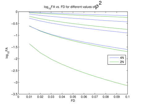
Figure 1: Compares the false alarm (FA) probabilities for the two detection statistics, ${\mathcal{F}_{4N}}$ and ${\mathcal{F}_{2N}}$, as a function of false dismissal (FD) probability, for several values of the squared signal strength, $\rho^{2}$. The blue curves are for ${\mathcal{F}_{4N}}$ and the green for ${\mathcal{F}_{2N}}$. From upper to lower, the squared signal strengths are $\rho^{2}=25,50,75,100$.

V Numerical results for one example search

To illustrate the utility of our ${\mathcal{F}_{pr}}$ statistic, in this section we present results for a simple, one-parameter family of examples (where the varied parameter is the strength of the embedded GW signal), and we compare the the effectiveness of ${\mathcal{F}_{pr}}$ and ${\mathcal{F}_{sc}}$.

We fix the number of intervals at $N=100$, and evaluate search effectiveness for signals with a range of total $\rho^{2}\equiv\sum_{i=1}^{N}\rho^{2}_{i}$. We will eventually consider a range of $\rho$, but for now imagine $\rho$ as fixed. For simplicity, in this example we will consider a case where the $\rho_{i}$ are the same for all $i$, so $\rho^{2}_{i}=\rho^{2}/N$, and where the $\Gamma^{i}_{ab}$ matrices are also the same for all $i$: $\Gamma^{i}_{++}=3$, $\Gamma^{i}_{+\times}=1=\Gamma^{i}_{\times+}$ and $\Gamma^{i}_{\times\times}=1$ for all $i$.

We decompose the measured signal $x^{i}$ into waveform plus noise,

$$x^{i}=h^{i}+n^{i}\,.$$ (41)

For each $i$, filtering the data with $H_{+}$ and $H_{x}$ produces two complex numbers: $c^{i}_{+}\equiv\big{(}{\bf x^{i}}\,|\,H_{+}\big{)}$ and $c^{i}_{\times}\equiv\big{(}{\bf x^{i}}\,|\,H_{\times}\big{)}$. Clearly, the measured signals $c^{i}_{\alpha}$ can be decomposed as

$$c^{i}_{\alpha} = \big{(}{\bf h^{i}}\,|\,H_{\alpha}\big{)}+\big{(}{\bf n^{i}}\,|\,H_{\alpha}\big{)}$$ (42)

$$\equiv g^{i}_{\alpha}+m^{i}_{\alpha}\,.$$ (43)

We simulate the noise piece $m^{i}_{\alpha}$ by taking random draws of (pairs of) complex numbers from a Gaussian distribution with covariance matrix

$$\big{<}{m^{i}_{\alpha}}^{*}m^{i}_{\beta}\big{>} \equiv \big{<}(H_{\alpha}\,|{\bf n^{i}}\,)\ \ <({\bf n^{i}}\,|\,H_{\beta})\big{>}$$ (44)

$$= (H_{\alpha}\ \,|\,H_{\beta})=\Gamma_{\alpha\beta}$$

Again for simplicity, we will consider a case where the $g_{i}^{\alpha}$ are the same for each $i$, modulo a random, complex phase factor. Our particular (and rather arbitrary) choice is

$$[\ g_{i}^{+}\,,\,g_{i}^{\times}]=(2N)^{-1/2}\rho\ [\ 2+\sqrt{6}\,,\,\sqrt{6}]\,e^{i\varphi^{i}}\,,$$ (45)

where the $\varphi^{i}$ are random phases drawn uniformly from $[0,2\pi)$. One easily checks that $\sum_{i=1}^{N}(h^{i}\,|\,h^{i})=\rho^{2}$. The inclusion of the $e^{i\varphi^{i}}$ terms reflects our goal of modeling a case where frequency evolutions of the tempate and the true signal are so mismatched that their relative phases jump significantly and randomly from one interval to the next. Choosing the $\varphi^{i}$ randomly corresponds to the ”worst-case scenario”, where the true-versus-template phase offsets show no pattern. In practice, we expect that the situation will often be much more favorable for searches: i.e., the phase offsets might very often be well fit by some low-order polynomial in time. In a later paper we plan to investigate the extent to which the time-evolution of the offsets can be fit by a few parameters, and how that information can be exploited to speed up other parts of the search.

Given one simulated data set $c^{i}_{\alpha}$ (200 complex numbers), we compute $2{\mathcal{F}_{pr}}$. We repeat for 10000 data sets to determine the distribution of $2{\mathcal{F}_{pr}}$, and calculate its mean $\big{<}2{\mathcal{F}_{pr}}(\rho)\big{>}$, standard deviation $\sigma_{pr}(\rho)$, skewness, and kurtosis. In practice, we find that the skewness and kurtosis are relatively small (as might be expected, since our N is large), so for the rest of this section we will approximate $p(2{\mathcal{F}_{pr}};\rho^{2})$ as simply a Gaussian with our measured mean and standard deviation. Given these distributions it is completely straightforward to determine the false alarm probability $FA$ for any threshold value $2{\mathcal{F}^{th}_{pr}}$, and to calculate the false dismissal probability $FD$ for any pair of $2{\mathcal{F}^{th}_{pr}}$ and $\rho^{2}$.

We expect that, in practical searches, ${\mathcal{F}^{th}_{pr}}$ will find its main use in hierarchical search algorithms, in which a very coarse search at relatively low threshold identifies candidates for further examination, and these are winnowed down in successive stages bc ; cgk . In this context, one generally wants a fairly small FD rate ($<1\%$, say), so as not to lose any events, and strongly prefers a very low FA probability, to reduce the computational cost of follow-ups. With this application in mind, in Figs. 2 and 3. we plot FA as a function of FD, for several values of $\rho^{2}$.

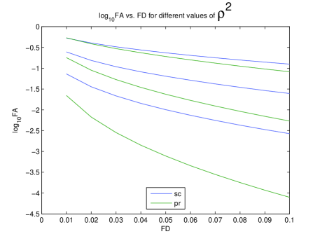
Figure 2: Compares the false alarm (FA) probabilites for the two detection statistics, ${\mathcal{F}_{sc}}$ and ${\mathcal{F}_{pr}}$, as a function of false dismissal (FD) probability, for several values of the (square of) the signal strength, $\rho^{2}$. The blue curves are for ${\mathcal{F}_{sc}}$ and the green for ${\mathcal{F}_{pr}}$. From upper to lower, the signal strengths are $\rho^{2}=75,100,125$.

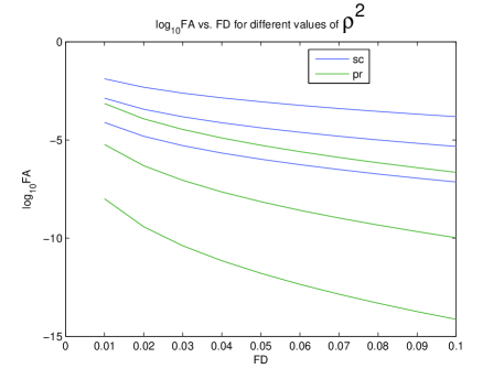
Figure 3: Same as in Fig. 2, except that, from the upper to lower curves, the signal strengths are $\rho^{2}=150,175,200$.

How much does employing ${\mathcal{F}_{pr}}$ increase the sensitity of a blind GW pulsar search? Obtaining a useful and accurate answer to this question is much more complicated than it might initially seem, since the most sensitive known search algorithms for GW pulsars are hierarchical searches bc ; cgk . These searches involve involve several stages, with successive stages ”ruling out” an ever-increasing fraction of the parameter space. We imagine that the most sensitive search–at some fixed, realistic computational cost–might use ${\mathcal{F}_{pr}}$ for only some of its stages. And while calculating ${\mathcal{F}_{pr}}$ clearly requires more floating point operations than calculating ${\mathcal{F}_{sc}}$, it is premature to compare these costs in a detailed way, since (i) there has as yet been no attempt to speed up our iterative relaxation scheme, and (ii) the extra information that comes with the phase offsets $\delta_{i}$ can presumably be used to speed up other parts of the search. Despite these difficulties we can obtain a rough estimate of the sensitivity improvement from using $\rho^{2}_{pr}$, as follows. We have seen that given some detection statistic ${\mathcal{S}}$, one naturally obtains a map from the total $\rho^{2}$ to curves in the $FA-FD$ plane. Let ${\mathcal{C}}({\mathcal{S}};\rho^{2})$ denote that curve. Then we can look for pairs $\rho^{2}_{pr}$ and $\rho^{2}_{sc}$ such that ${\mathcal{C}}({\mathcal{F}_{pr}};\rho_{pr}^{2})$ lies close to ${\mathcal{C}}({\mathcal{F}_{sc}};\rho_{sc}^{2})$. Three such pairs are shown in Fig. 4. We see that, in the most relevant portion of $FD-FA$ plane, ${\mathcal{C}}({\mathcal{F}_{pr}};140)$ lies close to ${\mathcal{C}}({\mathcal{F}_{sc}};170)$, ${\mathcal{C}}({\mathcal{F}_{pr}};160)$ lies close to ${\mathcal{C}}({\mathcal{F}_{sc}};200)$, and ${\mathcal{C}}({\mathcal{F}_{pr}};190)$ lies close to ${\mathcal{C}}({\mathcal{F}_{sc}};250)$. Thus, based on this example, we might estimate that using ${\mathcal{F}_{pr}}$ rather than ${\mathcal{F}_{sc}}$ affords an increase in sensitivity of $\sim 20-30\%$ in $\rho^{2}$, or $\sim 10-15\%$ in $\rho$. Clearly, to obtain a more reliable estimate we should perform a Monte Carlo simulation (based on random locations of the source on the sky, and random orientations of the GW pulsar’s spin axis). We plan to do this in follow-up work.

Comparing Fig. 1 to Fig. 2, we see that the sensitivity gain from replacing the detection statistic ${\mathcal{F}_{sc}}$ with ${\mathcal{F}_{pr}}$ is qualitatively similar to the gain from ${\mathcal{F}_{4N}}\rightarrow{\mathcal{F}_{2N}}$, but that the latter gain is greater (at least for our one numerical example, and for total SNR $\sim 10$). That may seem surprising, since in the former case we are eliminating $3N-3$ redundant parameters, while in the latter case we are eliminating only $2N$ redundant parameters. We conjecture that the main reason that the replacement ${\mathcal{F}_{sc}}\rightarrow{\mathcal{F}_{pr}}$ ”buys us less” in sensitivity is the following. In calculating ${\mathcal{F}_{2N}}$, the noise contributions from different intervals $i$ still get combined incoherently. However in ${\mathcal{F}_{pr}}$, the maximization over the phase offsets $\delta_{i}$ allows the noise contributions to combine coherently. Indeed for $\rho_{i}\lesssim 1$, the offsets $\delta_{i}$ are determined more by the noise than by the imbedded waveform. However we leave a thorough investigation of this effect to future work.

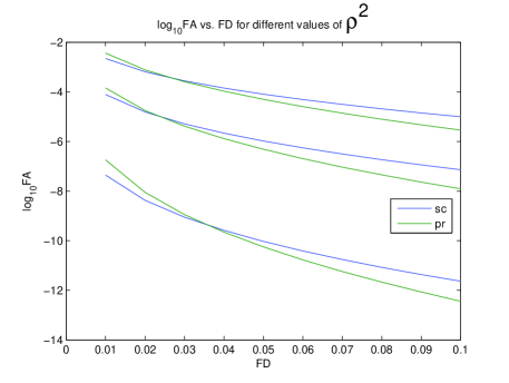
Figure 4: Similar to Figs. 2 and 3, except that here the sensitivity of the ${\mathcal{F}_{sc}}$ statistic is compared to that of ${\mathcal{F}_{pr}}$ at lower $\rho^{2}$. From upper to lower, the signal strengths for ${\mathcal{F}_{sc}}$ are for $\rho^{2}=140,160,190$.

VI Summary and Future Work

In this paper we defined a “phase-relaxed” ${\mathcal{F}}$-statistic, denoted ${\mathcal{F}_{pr}}$, to be used in cases where the total observation time is sufficiently long that straightforward calculation of the fully coherent ${\mathcal{F}}$-statistic over the relevant parameter space is computationally intractable. The calculation of ${\mathcal{F}_{pr}}$ takes as input the results from coherent searches over $N$ shorter time intervals. Our ${\mathcal{F}_{pr}}$ coincides with the fully coherent ${\mathcal{F}}$-statistic under the approximation that the phase offsets between template and imbedded signal are treated as an additional $N-1$ independent parameters. We also demonstrated one efficient, iterative method for calculating ${\mathcal{F}_{pr}}$. We regard our iterative method as an ”existence proof” for efficient algorithms. In future work we intend to explore variations on our basic method that we suspect would lead to substantial improvements in computational cost. We illustrated the use of ${\mathcal{F}_{pr}}$ in one simple family of examples, in which the sensitivity improvement (compared to ${\mathcal{F}_{sc}}$) was shown to be $\sim 10-15\%$.

Our example was based on the ”worst-case” assumption that where the phase offsets $\delta_{i}$ are completely random. In follow-on work we intend to examine the more realistic case where the $\delta_{i}$ are a (reasonably low-order) polynomial in time, and we plan to calculate the increased sensitivity based on a very large number of cases, in Monte Carlo fashion.

Other follow-on projects that we intend to work on include i) the development of new vetoes Itoh for instrumental artifacts, since, e.g., for true GW pulsars the parameters $(h_{0},\iota,\psi)$ calculated from the first half of the observation should be consistent with those calculated from the second half; ii) the use of the $\delta_{i}$ to quickly converge on improved estimates for the GW pulsar’s frequency and spindown parameters, and iii) the optimal use of ${\mathcal{F}_{pr}}$ in multi-stage, hierarchical searches.

Finally, while our primary interest in this paper has been the application of the ${\mathcal{F}_{pr}}$-statistic to GW pulsars, it has not escaped our notice that the same idea and formalism can be applied, with only trivial modifications, to searches for (quasi-circular, non-precessing) inspiraling binaries. With binaries, we expect ${\mathcal{F}_{pr}}$ to be most useful in those cases where the observed GW signal has a very large number of cycles; e.g., searches for neutron-star binaries by proposed GW detectors that have reasonable sensitivity at $\sim 1$ Hz, such as the Einstein Telescope, Decigo, or the Big Bang Observer.

- (1) P. Jaranowski, A. Krolak and B. F. Schutz, Phys. Rev. D 58, 063001 (1998).
- (2) C. Cutler & E. E. Flanagan, Phys. Rev. D 49, 2658 (1994).
- (3) C. Cutler and B. F. Schutz, Phys. Rev. D 72, 063006 (2005).
- (4) B. Abbott et al., Phys. Rev. D 80, 042003 (2009).
- (5) http://www.lsc-group.phys.uwm.edu/daswg/ .
- (6) V. Dergachev, Class. Quant. Grav. 27, 205017 (2010).
- (7) H. J. Pletsch, arXiv:1101.5396.
- (8) K.S. Thorne, in 300 Years of Gravitation, ed. S.W. Hawking and W. Israel (Cambridge University Press, Cambridge, 1987), pp. 330-458.
- (9) L. S. Finn and D. F. Chernoff, Phys. Rev. D 47, 2198 (1993).
- (10) S. Bonazzola & E. Gourgoulhon, Astron. Astrophys. 312, 675 (1996).
- (11) P. Brady, T. Creighton, C. Cutler & B. F. Schutz Phys. Rev. D 57, 2101 (1998).
- (12) P. Brady & T. Creighton, Phys. Rev. D 61, 082001 (2000).
- (13) C. Cutler, I. Gholami, & B. Krishnan, Phys. Rev. D 72, 042004 (2005).
- (14) Y. Itoh, M. A. Papa, B. Krishnan, and X. Siemens, Class. Quant. Grav. 21, S1667 (2004).