The MIPSGAL view of supernova remnants in the Galactic Plane

Abstract

We report the detection of Galactic supernova remnants (SNRs) in the mid-infrared (at 24 and 70 $\micron$), in the coordinate ranges $10^{\circ}<l<65^{\circ}$ and $285^{\circ}<l<350^{\circ}$, $|b|<1^{\circ}$, using the Multiband Imaging Photometer (MIPS) aboard the Spitzer Space Telescope. We search for infrared counterparts to SNRs in Green’s catalog and identify 39 out of 121, i.e., a detection rate of about 32%. Such a relatively low detection fraction is mainly due to confusion with nearby foreground/background sources and diffuse emission. The SNRs in our sample show a linear trend in [F₈/$F_{24}$] versus [F₇₀/$F_{24}$]. We compare their infrared fluxes with their corresponding radio flux at 1.4 GHz and find that most remnants have ratios of 70 $\micron$ to 1.4 GHz characteristic of SNRs (with the exception of a few which have ratios closer to those of H II regions). Furthermore, we retrieve a slope close to unity when correlating infrared (24 and 70 $\micron$) with 1.4 GHz emission. Our survey is more successful in detecting remnants with bright X-ray emission, which we find is well correlated with the 24 $\micron$ morphology. Moreover, by comparing the power emitted in X-ray, infrared and radio, we conclude that the energy released in the infrared is comparable to the cooling in the X-ray range.

1. Introduction

With the help of Galactic surveys (e.g., Arendt, 1989, Saken et al., 1992), our understanding of the infrared (IR) energetics, morphology and evolution of supernova remnants (SNRs) has increased substantially in the past decades. However, even at IRAS (Infrared Astronomical Satellite) resolution, confusion with other IR sources in the Galactic plane is a limiting factor that can prevent a clear picture from emerging. Such confusion, for example, can make the correct assessment of ejecta dust masses for Type II SNRs difficult, a key factor for interpreting high redshift dust in the Universe (Sibthorpe et al., 2010, and references therein). Infrared emission from SNRs can also provide insight into the radio-IR correlation of external galaxies (Helou et al., 1985). Additionally, the study of dust re-emission is relevant for determining the cooling rate of SNRs, an important quantity that shapes their evolution (Dwek, 1987).

In this paper, we search for counterparts of SNRs in the mid-infrared (at 24 and 70 $\micron$) using the higher resolution Spitzer data obtained with the Multiband Imaging Photometer (MIPS), in the coordinate ranges $10^{\circ}<l<65^{\circ}$ and $285^{\circ}<l<350^{\circ}$, $|b|<1^{\circ}$, complementing the work of Reach et al. (2006). We also briefly explore the relation of SNRs IR fluxes with other wavelength ranges, such as the radio and the X-ray.

The structure of this paper is as follows: In §1.1, we review previous Galactic infrared surveys and their detection rates. In §1.2, we discuss SNR emission mechanisms which can contribute in the mid-infrared regime. In §2, we describe the mid-infrared, radio and X-ray data used in this work. In §3, we report the MIPS detections. A discussion of SNR identifications, derived color ratios and radio and X-ray to infrared ratios follows in §4. Finally, in §5, we summarize our findings. Details on each detected SNR can be found in the appendix.

1.1. Previous Galactic Infrared Surveys

Using the Galactic Legacy Infrared Mid-Plane Survey Extraordinaire, GLIMPSE (Benjamin et al., 2003; Churchwell et al., 2009), Reach et al. (2006) searched the Galactic Plane for infrared counterparts to known SNRs. Out of 95 objects, 18 were clearly detected, a detection rate of about 20%. Previous searches were conducted using the IRAS all-sky survey. Within the GLIMPSE surveyed area, Arendt (1989) obtained a detection rate of 17% and Saken et al. (1992) 18% (Reach et al., 2006). In the present study, we identify 39 out of 121, i.e., a detection rate of about 32%.

1.2. SNR infrared emission mechanisms

The IR part of the spectral energy distribution (SED) of SNRs can result from multiple sources ranging from dust (either stochastically or thermally heated), atomic/molecular line emission, PAH (polycyclic aromatic hydrocarbon) emission, and even synchrotron emission. In fact, the amount of the latter emission can vary substantially and is dependent on the type of remnant. In plerion remnants such as the Crab Nebula (Strom & Greidanus, 1992), it accounts for about 90% of the mid-infrared flux density (at 25 $\micron$). In contrast, about 2% of the mid-infrared flux density (at around 25 $\micron$) in Cas A is due to synchrotron emission (Sibthorpe et al., 2010).

Dust emission is expected to be a substantial component of the IR emission of SNRs since their spectra is well fitted by one or more thermal dust populations, as revealed by previous infrared surveys (IRAS; Arendt, 1989, Saken et al., 1992), or by stochastic heating of the grains, as proposed by Hines et al. (2004) to explain the mid-infrared emission from Cas A. The dust is heated by charged particles in hot plasma generated by shocks (e.g., Dwek & Werner, 1981, Dwek, 1987, Dwek & Arendt, 1992). Direct evidence for the shock-heated plasma is provided by X-ray observations in the continuum, and X-ray lines are a good diagnostic of high energy interactions and abundances (Vink, 2004). While for the majority of SNRs, the observed dust emission is thought to originate from the interaction of the shockwave with the surrounding interstellar medium (ISM; e.g., Douvion et al., 2001, Borkowski et al., 2006, Williams et al., 2006a, Blair et al., 2007), evidence of SNRs with ejecta dust is scarce (e.g., Arendt et al., 1999) even with the help of higher resolution IR telescopes such as ISO and Spitzer. However, observations with the Spitzer Infrared Spectrograph (IRS) (Rho et al., 2008) of the young remnant Cas A have pointed to the presence of a large hot dust continuum peaking at 21 $\micron$, from ejecta dust formed through condensation of freshly synthesized heavy elements. This component has temperatures ranging from 60 to 120 K. Furthermore, recent far-infrared and sub-millimeter work (Sibthorpe et al., 2010) on the same remnant, also suggested the existence of a ‘tepid’ ($\sim 35$ K) central dust component in the ejected material (see also Barlow et al., 2010).

Observational evidence for the importance of IR lines has been provided by multiple SNRs spectroscopic studies which identified a plethora of lines from elements such as Fe and O (e.g., Oliva et al., 1999b; Reach et al., 2002). Much of the infrared line emission seen in SNRs results from the interaction of the blastwave with the surrounding environment where they are born as the shocked gas cools down. For example, IC443 is encountering an atomic region at the northeast side and a molecular cloud at the southern border (e.g., Rho et al., 2001). Spectral observations by Oliva et al. (1999a) on the north of the remnant revealed that most of the emission at 12 and 25 $\micron$, previously surveyed with IRAS, was in fact due to ionized line emission (e.g., [Fe II]) with only a small contribution from dust. Because optical spectra also showed strong collisionally excited fine structure atomic lines (Fesen & Kirshner, 1980), the infrared line emission is not unexpected. Likewise, for the ’optically bright regions’ in N49, an old remnant in the Large Magellanic Cloud (LMC), Williams et al. (2006b) found that IR line emission can be a substantial fraction of the total IR flux, up to 80% at 24 $\micron$. On the south of IC443, however, the spectrum is dominated by the H₂ pure rotational lines S(2) through S(7) (Cesarsky et al., 1999), once again with a faint dust continuum. Moreover, Troja et al. (2006) found a good agreement between the soft X-ray emitting plasma and the radio/optical structure on the northeastern part of the remnant where the plasma density is highest. Such energetic encounters change the morphology of the neighboring ISM and of the remnant itself thereby creating prominent emission lines (e.g., molecular hydrogen) which can be detected in the infrared. OH masers (in particular, the 1720 MHz line) are also good tracers of the remnant encounter with dense molecular regions with 10% of Galactic SNRs showing associated masers (Wardle & Yusef-Zadeh, 2002 and references therein).

The existence of infrared emission associated with PAHs in SNRs was first observed in a LMC remnant by Tappe et al. (2006). Plus, evidence for such emission in some Galactic SNRs has also been shown through near-infrared color-color ratios by Reach et al. (2006). This is likely excitation of PAHs from the ISM, rather than PAHs from supernova dust.

2. Data Used

2.1. Infrared Data

Infrared data used in this paper originates from two Spitzer surveys: GLIMPSE using the Infrared Array Camera (IRAC) and MIPSGAL (survey of the inner Galactic plane using MIPS, Carey et al., 2009). Both surveys cover the Galactic coordinates $10^{\circ}<l<65^{\circ}$ and $285^{\circ}<l<350^{\circ}$, $|b|<1^{\circ}$.

2.1.1 MIPSGAL

The MIPS wavelength coverage is approximately 20 to 30 $\micron$ at ch 1 (24 $\micron$) and 50 to 100 $\micron$ at ch 2 (70 $\micron$), thus covering a potentially rich set of diagnostic lines and dust emission features (see Fig. 1). In the 24 $\micron$ bandpass, the classic [O IV] 25.9 and [Fe II] 26.0 $\micron$ tracers can be quite strong (e.g., Oliva et al., 1999a; Noriega-Crespo et al., 2009), and likewise [O I] 63 and [O III] 88 $\micron$ (e.g., Rho et al., 2001) within the 70 $\micron$ bandpass. Other standard shock excitation tracers, like [Ne II] 12.81 or [Si II] 34.8 $\micron$, are unfortunately not included within the IRAC or MIPS bandpasses. Nevertheless, when dust is present, it is the dominant component of the IR radiation at 24 and 70 $\micron$ (see Fig. 1).

Although the 24 $\micron$ data delivered by the Spitzer Science Center in their Post-BCD products are of a very high quality, the MIPSGAL pipeline was designed to enhance the data a step further. The details are described in Mizuno et al. (2008), but briefly the pipeline: (1) carefully deals with saturated and non-saturated data, a key issue in the Galactic Plane; (2) removes a series of artifacts, the most common being a column-to-column jailbar striping, plus (3) that of short-duration afterimage latencies, (4) long-duration responsivity variations, and (5) background mismatches. The MIPSGAL observations were designed to be a 24 $\micron$ survey as the high background levels of the Galactic plane at longer wavelengths saturated the 160 $\micron$ detectors and placed the 70 $\micron$ at a fluence level not well characterized. Since MIPS takes data simultaneously at 70 and 160 $\micron$, and that at 70 $\micron$ at first sight looks reasonable, then a concerted effort has been invested by the MIPSGAL team to improve its quality. The specific steps of the 70 $\micron$ pipeline are described in Paladini et al. (in preparation), but the main issue is to mitigate the effect of the non-linear response of the Ge:Ga photoconducting detectors. Their standard behavior leads to striping of the images, sudden jumps in brightness and a large uncertainty in the calibration for bright sources and regions. The MIPSGAL 70 $\micron$ pipeline reduces these effects and decreases the calibration uncertainties to a level of $\sim$15$\%$. This uncertainty on the absolute calibration of the extended emission is consistent with that determined by the MIPS team in their calibration at 24 and 70 $\micron$ (Engelbracht et al., 2007; Gordon et al., 2007). The adopted uncertainty in calibration for MIPS 24 $\micron$ is 10% . For the 70 $\micron$ fluxes, the main errors come from uncertainties in the background estimation and calibration errors (we adopt a conservative value of 20%). Moreover, we have used the 24 $\micron$ point source subtracted data. For details in the point source removal procedure see Shenoy et al. (in preparation). Point source sensitivities are 2 and 75 mJy (3$\sigma$) at 24 and 70 $\micron$, respectively. The resolution of the 24 $\micron$ data is $6^{\prime\prime}$ while for 70 $\micron$ it is $18^{\prime\prime}$.

2.1.2 GLIMPSE

At the IRAC bands (Reach et al., 2006, in particular Fig. 2) one expects to find a wealth of atomic lines, including Br$\alpha$ (4.05 $\micron$), Pf$\beta$ (4.65 $\micron$), [Fe II] (5.34 $\micron$), and [Ar II] (8.99 $\micron$), among others, plus the molecular S(13) through S(4) H₂ rotational lines, and CO transitions at 4-5 $\micron$. This is very much the case in IC 443 (Neufeld & Yuan, 2008; Cesarsky et al., 1999). We use primarily the 8 $\micron$ images from IRAC. Occasionally, other channels are also used in order to constrain the possible emission mechanisms. The 4.5 $\micron$ channel provides a valuable diagnostic of shocked molecular gas (e.g., Reach et al., 2006). At these wavelengths, our measured flux represents an upper limit since star contamination is present. We adopt a conservative value of 10% for the calibration error given the vagaries in color correction plus measurement errors. The IRAC sampling is $1.2^{\prime\prime}$ but the 8 $\micron$ resolution is about $2^{\prime\prime}$.

2.2. Ancillary Data

Most of the supernova remnants in Green’s catalog (Green, 2009a) are discovered using radio observations. By comparing the emission in at least two different radio wavelengths, one can calculate the spectral index and thus distinguish the kind of emission produced (thermal or non-thermal). In the case of SNRs, we expect to find a spectral index which is characteristic of synchrotron radiation. In contrast, H II regions show a flat spectrum (when optically thin) which is indicative of free-free emission. The SNR radio emission is associated with regions where shock-induced particle acceleration take place within the source.

In addition to data in Green’s catalog, the following radio data sets are used for comparison with the infrared images: VLA (Very Large Array) archival data at 20 and 90 cm, available from the Multi-Array Galactic Plane Imaging Survey (MAGPIS; Helfand et al., 2006) website, VGPS (VLA Galactic Plane Survey; Stil et al., 2006) at 21 cm and MOST (Mongolo Observatory Synthesis Telescope; Whiteoak & Green, 1996) at about 36 cm.

Wide band (300-10000 eV) X-ray images from the Chandra Supernova Remnant Catalog archive are also used for comparison. X-ray emission locates the shock heated plasma, including the important reverse shock in the interior region.

3. Detections of SNRs

To describe the amount of (or lack of) infrared emission from SNRs in our sample, we use a similar classification scheme to the one adopted by Reach et al. (2006). Detection levels are characterized as follows: (1) detected, (2) possible detection, (3) unlikely detection and (4) not detected (see Table 1). Level 1 detections have a good positional match between the infrared contours and those at other energies (radio or X-ray). Level 2 detections display infrared emission within the remnant region but confused with cirrus or nearby H II regions. Level 3 detections show the presence of some infrared emission which does not seem to be correlated with the remnant, although source confusion prevents a clear assessment of the emission origin. Level 4 is characterized by the absence of infrared emission within or nearby the contours of the radio remnant.

Out of a sample of 121  possible radio remnants, 39 are level 1 detections, a detection rate of 32% compared to 18% with GLIMPSE. A few examples of level 1 detections are shown in Fig. 2. The MIPSGAL sensitivity at 24 $\micron$ matches very well that of IRAC at 8 $\micron$ (Carey et al., 2009; Benjamin et al., 2003). The fact that we can identify many more SNRs than with IRAC could potentially be due to an extinction effect (lower at 24 $\micron$ than at 8 $\micron$ by 40$\%$, Draine, 2003). However, it is far more plausible that it could simply be the details of how SNRs emit. In the case of SNRs interacting with the ISM where shocks modify the dust grain size distribution (e.g., Guillard et al., 2010), 24 $\micron$ continuum emission (due to Very Small Grains, VSGs) rises while at 8 $\micron$ the emission by stochastically heated PAHs is not as strong.

We calculate flux densities at 8, 24, and 70 $\micron$ for SNRs which show obvious infrared counterparts (level 1 detections). The aperture size used for the flux derivations is, in some cases, different from the one listed at radio wavelengths (see Table 2). This is done in order to account for the different morphologies a remnant can have in various wavelength ranges. Furthermore, there are cases where the SNR is nearby other unrelated extended Galactic sources whose contamination can lead to an overestimate of the infrared flux (e.g., diffuse Galactic emission and H II regions). To avoid such problems, we examined the MIPS images overlaid with contours from other wavelengths to help constrain the location and shape of the SNR infrared emission; however, such discrimination is not always well achieved. Another issue that arises, especially when dealing with Galactic plane images such as these, is the presence of unrelated infrared emission along the line of sight. This confusion can hinder the detection of SNRs as demonstrated by Arendt (1989) and Saken et al. (1992).

Flux densities of the detected remnants were obtained using either a circular or elliptical aperture with a background removed. The background was determined using the median value of the sky brightness around the remnant via two methods. We used an annulus around the source for cases where the external source contamination in the neighborhood is negligible. However, that method was often not feasible due to considerable overlap of sources (extended or point-like) with the periphery of the SNR. For those cases, the sky brightness was estimated with a user-selected region characteristic of the local background emission. In order to quantify the magnitude of background variations, we measured the surface brightness on several regions around one of the faintest 24$\micron$ SNR, G21.8-0.6. We used aperture sizes similar to the one used for the remnant and found that the standard deviation relative to the mean background value across the field, for our three wavelengths are of the order of 12% (8 $\micron$), 10% (24 $\micron$) and 20% (70 $\micron$).

Another consideration for photometry measurements is point source contamination, especially at 8 $\micron$ (as discussed in § 2.1.2). Finally, since we are dealing with spatially extended emission, we applied corrections to the 8 $\micron$ estimates to account for internal scattering in the detectors as instructed by the IRAC data handbook. The ‘infinite’ radius aperture is most appropriate for the angular extent of the remnants; we multiplied the surface brightness measurements by 0.74.

4. Discussion

4.1. Comparison of detections with previous infrared surveys

Out of the previous 18 detections (level 1) using GLIMPSE (Reach et al., 2006), we confirm 16 at the same level with MIPSGAL (Table 1). The remaining two remnants are confused with the background and are reported as possible detections in our analysis. Of the other 23 (level 1) infrared counterparts found in this work, 10 are not in the initial sample from Green’s catalog used by Reach et al. (2006) and the remaining 13 are mostly bright X-ray remnants which seem to be brighter at 24 $\micron$. Regarding the SNRs identified by Arendt (1989), all of their level 1 detections are also seen in MIPSGAL with the exception of G12.0-0.1 and G54.1+0.3 which are both level 3 in the MIPS data. Comparing with Saken et al. (1992), six SNRs have been detected in common (level 1). They also reported a level 1 detection of 8 others, which we classify as level 2 or 3. Again, we observe that these cases are mostly regions where there is a large contamination by nearby or overlapping H II regions making a clear identification challenging even at the superior Spitzer resolution.

4.2. Lack of infrared signature

Given the strong ambient emission in the inner Galactic plane, it is not surprising that many SNRs, either too big or too old, and having low infrared surface brightness, do not have an identifiable infrared signature. Also, as noted by Williams et al. (2006b), the environs in which SNRs are encountered need to be sufficiently dense to promote collisional heating of the dust, thus making it distinguishable. Examples of non-detections in this survey are G18.1-0.1 and G299.6-0.5.

4.3. Color-color Diagrams

Table 2 shows flux densities (at 8, 24 and 70 $\micron$) and color ratios for the detected remnants. Figure 3 contains a logarithmic plot of [F₈/F₂₄] versus [F₇₀/$F_{24}$] for which SNRs are detected as a whole (see last column of Table 2).

Two other SNRs are plotted: for Cas A, values are retrieved from Hines et al. (2004) and for IC443 from Noriega-Crespo et al. (in preparation). The data show a linear trend with a slope of $1.1\pm 0.2$: remnants with a low [F₈/F₂₄] ratio statistically have a low [F₇₀/F₂₄] ratio. Furthermore, there seems to exist an age effect, with older remnants (such as IC443 and W44) showing higher [F₇₀/F₂₄] and [F₈/F₂₄]. The opposite seems to be more characteristic of younger remnants, such as Cas A, Kes 73 and G11.2-0.3.

In some remnants, infrared emission is only detected in certain parts inside the radio/X-ray contours. Figure 4 shows surface brightness ratios of these localized regions. To assess the mechanism of the infrared emission, we also calculate surface brightnesses for regions of SNRs known to be either interacting with neighboring molecular regions (such as the BML region in 3C391) and/or that show molecular emission lines (such as W49B) or known to have ionic lines (such as 3C396). For this exercise, we used regions of some remnants for which the main emission mechanism had previously been identified by Reach et al. (2006) (see their Fig. 22). These are also identified in the SNR figures in the appendix. Remnants with colors characteristic of ionic shocks seem to occupy the lower left part of the [I₇₀/I₂₄] versus [I₈/I₂₄] diagram, while remnants whose colors are consistent with molecular shocks and photodissociation regions are found in the upper right part. However, given the small number of examples and the fact that all three passbands (8, 24 and 70 $\micron$) contain dust emission and lines, we suggest that the [I₇₀/I₂₄] and [I₈/I₂₄] color ratios are not a completely secure method of distinguishing between different emission mechanisms.

We plot some other color ratios for comparison. The locus for pure synchrotron is for spectral index of 0.3 to 1 . For the diffuse ISM, we used the color ratios obtained by Compiègne et al. (2010) for two regions (with different abundances of very small grains) in the Galactic plane at a longitude of approximately $59^{\circ}$. We have also included color ratios for evolved H II regions (found near Galactic longitudes of $35^{\circ}$; Paladini et al. (in preparation)).

Are the color ratios [F₇₀/$F_{24}$] and [F₈/F₂₄] good discriminators between such very different regions? Based on Figure 4, the plotted colors of individual evolved H II regions often seem indistinguishable from SNRs using Spitzer colors. However, the overall trend for SNRs is displaced from the H II regions and covers a broader range of colors. This is similar to what Arendt (1989) found for older SNRs and compact H II regions using IRAS colors.

Although line contamination is significant for radiative remnants, for younger ones the majority of the IR emission should be due to dust grains. For instance, for RCW 103 (age approximately 2000 yr; Carter et al., 1997) we calculate the ratio of line emission (using ISO data) versus dust continuum within MIPS filters. We find that line emission contributes about 6% and 3% of the observed flux at 24 and 70 $\micron$, respectively.

If emission from the remnants comes primarily from shocked hot dust, then we can derive the dust temperature just by assuming a simple modified blackbody emission. If dust has a thermal spectral energy distribution

$$S{{}_{\nu}}\propto~{}B{{}_{\nu}}(T)~{}\nu^{\beta}\,,$$ (1)

where $\beta$ is the dust emissivity index (which depends on the dust composition, $\beta\sim 1$ to 2), then flux ratios imply certain temperatures. Figure 3 shows temperatures based on the [F₈/$F_{24}$] and [F₂₄/$F_{70}$] ratios. The latter flux ratio yields dust temperatures for our SNR sample ranging between 45 and 70 K for $\beta=2$ and from 50 to 85 K for $\beta=1$. This is a very crude estimate of the dust temperature given that we are just considering one population of dust grains in temperature equilibrium when it is far more likely that there are several populations plus non-equilibrium emission. Applying the same simple dust model to the [F₈/$F_{24}$] ratio, we obtain temperature values higher than 145 K (for $\beta=2$) with younger SNRs having color temperatures lower that older remnants. This trend is similar to what was obtained by Arendt (1989) using color temperatures based on the IRAS 12 to 25 $\micron$ ratio. The infrared colors are not well explained by a single equilibrium dust temperature and atomic and molecular line emission as well as PAHs might significantly contribute to the infrared emission for SNRs.

However, assuming that the infrared emission at 24 and 70 $\micron$ is cospatial, entirely due to dust, and well fitted by a single temperature modified blackbody, then SNR dust masses are given by the following equation:

$$M{{}_{\mathrm{dust}}}=\frac{d{{}^{2}}~{}F{{}_{\mathrm{\nu}}}}{{\kappa}{{}_{\mathrm{\nu}}}~{}B{{}_{\mathrm{\nu}}(T{{}_{\mathrm{dust}}})}}\,,$$ (2)

where $d$ is the distance to each SNRs, $F{{}_{\nu}}$ is the flux density and $\kappa{{}_{\nu}}$ is the dust mass absorption coefficient. For the dust mass absorption coefficient, we use the diffuse ISM model by Li & Draine (2001) which consists of a mixture of amorphous silicate and carbonaceous grains. Distances are retrieved from Green’s catalog. Results are reported in Table 3. Note that these derived dust masses, based on the 24 and 70 $\micron$ fluxes from MIPS, are overestimated given the probable contamination of these fluxes by line emission which can be substantial in radiative remnants. Even in the case where all of the flux in these bands is due to dust, mass estimates are based on a single color temperature (24/70) which can be reasonable for younger remnants but not ideal for older remnants given that their IR SED generally requires more that one dust population (Arendt, 1989; Saken et al., 1992).

4.4. Infrared to radio (1.4 GHz) ratio

According to Haslam & Osborne (1987), the comparison between mid-infrared (60 $\micron$ from IRAS) and radio continuum (11 cm) emission is a good diagnostic for distinguishing between thermal from non-thermal radio emitters (see also (Fuerst et al., 1987) and (Broadbent et al., 1989)). H II regions are shown to have infrared to radio ratios of the order of $\geq 500$ while ratios for SNRs are thought to be lower than 20. Moreover, Whiteoak & Green (1996) using MOST found that SNRs have a ratio of infrared (60 $\micron$) to radio (843 MHz or 36 cm) of $\leq 50$ while H II regions have again ratios of the order of 500 or more.

We use the 1 GHz flux densities provided in Green’s catalog (Green, 2009a). Those values were converted to 1.4 GHz (21 cm) flux densities using the spectral indices quoted in the same catalog. We compare those to the 24 and 70 $\micron$ emission from MIPSGAL. Figure 5 shows the spread in the ratio of the infrared to radio for the detected SNRs. Note that these ratios are often defined by $q{{}_{\mathrm{IR\lambda}}}=\log(F{{}_{\mathrm{IR\lambda}}}/F{{}_{\mathrm{21cm}}})$ where F_IRλ and F_21cm are the flux densities (in Jy) at specific mid-infrared wavelengths and in the radio.

There seems to be a group with ratios (or high $q{{}_{\mathrm{24}}}$ and $q{{}_{\mathrm{70}}}$) similar to those of H II regions. In particular, we suggest that the morphology of the remnant G23.6+0.3 (and possibly G14.3+0.1) resembles more closely an H II region and so whether it is a SNR should be re-considered. See also its infrared colors compared to H II regions (Figs. 3 and 4). Image in Figure 21 (and 13) clearly shows a composite infrared emission, with the 24 $\micron$ (probing hot and small particles) matching the radio, while the 8 and 70 $\micron$ emission do not spatially coincide with the 24 $\micron$. In particular, the 8 $\micron$ appears as an outer layer which marks the transition between the ionized region and colder gas. The 70 $\micron$ emission is also seen along the same location as the 8 $\micron$, which is consistent with the premise that we are now probing a colder dust population.

There is a strong empirical correlation between infrared and radio emission (at 1.4 GHz) found in spiral galaxies (Helou et al., 1985). The radio emission in this range is thought to be mainly due to synchrotron emission with only 10% is attributed to thermal bremsstrahlung produced by H II regions (Murphy, 2009 and references therein). In our Galaxy and other local star forming galaxies, the bulk of the mid and far-infrared arises from warm dust associated with star forming regions. In older systems, things are more complicated due to cold cirrus and evolved stars (e.g., AGBs). We look for a similar correlation using the infrared and radio emission from our SNR sample. We estimate the mid-infrared emission as the sum of the integrated emission in each MIPS passband (24 and 70 $\micron$) and obtain an integrated mid-infrared flux F_MIR in units of W/m² (see Helou et al., 1985). The F_MIR is an approximation (underestimate) of the mid-infrared bolometric flux (given that the bandpasses of 24 and 70 $\micron$ filters do not overlap). Figure 6 shows the correlation between infrared and 1.4 GHz non-thermal radio flux. The slope of the correlation is $1.10\pm 0.13$ when combining all data (plus IC443). Again, two distinct populations seem to exist, an upper main trend and a lower one. Using only the lower one (i.e., objects which have 70 $\micron$ to 1.4 GHz ratios closer to H II regions and high values of $q{{}_{\mathrm{24}}}$ and $q{{}_{\mathrm{70}}}$ in Fig. 5), we obtain a slope of $0.93\pm 0.13$ while for the upper trend we get $0.96\pm 0.09$.

The correlation with the slope fixed to unity leads to the dimensionless parameter $q{{}_{\mathrm{MIR}}}$ (Helou et al., 1985) which represents the ratio of mid-infrared to radio and is defined as

$$\small q{{}_{\mathrm{MIR}}}\equiv\mathrm{\log}\Big{(}\frac{F{{}_{\mathrm{MIR}}}}{3.75\times 10^{12}~{}\mathrm{Wm^{-2}}}\Big{)}-~{}\mathrm{\log}\Big{(}\frac{F~{}{{}_{\mathrm{1.4~{}GHz}}}}{\mathrm{Wm^{-2}~{}Hz^{-1}}}\Big{)}\,.$$ (3)

Our results show that remnants from the lower trend population in Figure 6 have $q{{}_{\mathrm{MIR}}}$ larger than 2.06 (up to 2.60). The other group has $q{{}_{\mathrm{MIR}}}$ ranging from 0.06 and 1.41. Specific $q$ values for each remnant are displayed on Table 4. For reference, a previous study by Bell (2003) reported a median value of $q{{}_{\mathrm{TIR}}}$ (i.e., the ratio of the total 8-1000 $\micron$ IR luminosity to the radio power) of $2.64$ for a sample of 162 galaxies. But note this would be higher because it is based on the total IR emission.

Table 5 reports on the average and dispersion of the monochromatic $q{{}_{\mathrm{8}}}$, $q{{}_{\mathrm{24}}}$ and $q{{}_{\mathrm{70}}}$ parameters for the two trends. For comparison, a study of extragalactic VLA radio sources by Appleton et al. (2004) obtained $q{{}_{\mathrm{24}}}=0.84$ and $q{{}_{\mathrm{70}}}=2.15$ while Boyle et al. (2007) found $q{{}_{\mathrm{24}}}=1.39$ for somewhat fainter galaxies. Later on, Seok et al. (2008) using AKARI data for some LMC SNRs compared the ratio of 24 $\micron$ to radio fluxes; their correlation implies $q{{}_{\mathrm{24}}}=0$. If SNRs are the sole contributors of synchrotron emission in a star-forming galaxy, then by comparison with the above $q{{}_{\mathrm{24}}}$’s for galaxies they concluded that about 4 to 14% of the 24 $\micron$ emission in galaxies is due to SNRs. By doing a similar exercise using the upper trend remnants, for which $q{{}_{\mathrm{24}}}=0.39$ (see Table 5), we find that 10 to 35% of the 24 $\micron$ galactic emission seen would be due to the remnants. Likewise, at 70 $\micron$ that contribution would be 11%. The rest would be due to dust heated in H II and photo-dissociation regions, as well as diffuse emission.

4.5. High energy emission from SNRs

In this section, we explore the relationship between the infrared and X-ray energetics of SNRs. Shocks produce hot plasma whose thermal energy is transferred to the dust grains via collisions and then re-emitted in the infrared (Ostriker & Silk, 1973; Draine, 1981; Dwek, 1987). Heating up the dust grains takes energy from the X-ray gas, thus cooling it and a good tool to measure this transfer of energy is the ratio of infrared to X-ray power, usually referred to as IRX (Dwek et al., 1987), which compares dust cooling (gas-grain collisions) with X-ray cooling (continuum and lines). The gas cooling function increases at lower plasma temperatures given that more lines become available due to recombination. On the other hand, at high temperatures of around $10^{7}$ K, most of the energy is released through the bremsstrahlung continuum (Raymond et al., 1976). Assuming that line emission in the infrared is not energetically significant compared to the X-ray lines, then most of the line cooling must happen in the X-ray domain. This implies that if the observed powers in the infrared and X-ray are comparable then dust must be the essential contributor to the cooling in the infrared.

Table 6 shows the values of IRX for a sample of SNRs. The total X-ray fluxes (with energy range from 0.3 to 10 keV) were retrieved from the Chandra Supernova Remnant Catalog. Infrared flux densities (in Jy) were measured for regions approximately matching those in the X-ray. We obtain the IR flux by integrating under the SED using simple linear interpolation in log space plus $\nu$F$\nu$ constant across the 24 $\micron$ passband. Also, note that the flux densities used in this analysis are not corrected for extinction. For our sample, IRXs range from about 1.6 for remnant RCW103 to 240 for W44.
These data are presented as SEDs in Figure 7, in the logarithmic form $\lambda F{{}_{\lambda}}$ vs. $\lambda$ which is convenient for assessing the energetics. The radio values are obtained from Green’s catalog (Green, 2009a). We also include Cas A and IC443 for comparison. Their infrared flux densities are taken from Hines et al. (2004) and Noriega-Crespo et al. (in preparation) while the X-ray fluxes are from the Chandra Supernova Remnant Catalog and Dwek et al. (1987), respectively. In Figure 7 the remnants are sorted according to increasing age (see Table 6). Although the ages for some remnants are uncertain, this Figure shows that hot dust grain cooling (24 $\micron$) tends to be the most important contributor in early phases of the remnant, while in the later stage the warm dust traced by the 70 $\micron$ emission is the main contributor to plasma cooling. It also appears that older remnants tend to have greater IRXs. This can potentially be either due to an increase in the dust-to-gas ratio and/or a change in the size distribution favoring smaller sizes.

5. Conclusion

We have compiled a catalog of SNRs detected within the MIPSGAL survey at 24 and 70 $\micron$, with complementary measurements at 8 $\micron$ from the GLIMPSE survey. In order to better assess the nature of the detected infrared emission, we have compared it with radio and X-ray data. Our main findings are the following:

• The detection rate of SNRs given the MIPSGAL sensitivity is 32$\%$, 39 out of the 121 candidates from Green’s SNR catalog and higher than any previous infrared survey.

• We find a linear trend (slope $=1.1\pm 0.2$) in the logarithmic relationship between [F₈/F₂₄] versus [F₇₀/$F_{24}$]. If there is indeed an age effect, then the youngest SNRs will have the lowest [F₈/F₂₄] and [F₇₀/F₂₄] ratios.

• The [I₇₀/I₂₄] and [I₈/I₂₄] color ratios provide a method of distinguishing between different emission mechanisms. This is not completely secure and the color ratios of some SNRs overlap with those of H II regions.

• Assuming a simple modified blackbody model (at 24 and 70 $\micron$), we retrieve SNRs dust temperatures which range from 45 to 70 K for a dust emissivity of $\beta=2$.

• Using the previous color temperature (T_24/70), we find rough estimates of dust masses ranging from 0.02 to 2.5 M_☉. Note that the dust masses obtained here may be overestimated given the possible contribution of line emission to the MIPS fluxes.

• We also compare infrared fluxes with their corresponding radio fluxes at 1.4 GHz and find that most of the remnants have ratios of 70 $\micron$ to 1.4 GHz characteristic of SNRs, although six (about 18% of the detected sample) have ratios closer to those found for H II regions.

• The slope of the logarithmic correlation between ‘total’ mid-infrared flux (24 and 70 $\micron$) and the 1.4 GHz non-thermal radio flux is close to unity (1.10) as found for galaxies. $q{{}_{\mathrm{MIR}}}$ values were calculated for each fully detected remnant and they range between approximately 0.06 and 2.60.

• Whether the strong 24 $\micron$ emission is the result of line emission or hot dust, it is clear that there is a good morphological association of the 24 $\micron$ and X-ray features in bright X-ray remnants. The mechanism for the 24 $\micron$ emission for these remnants is most likely grains heated by collisions in the hot plasma. The morphology of this mid-infrared emission is also generally distinct from the other infrared wavelengths which implies that the emission at 8 and 70 $\micron$ has a different origin.

• We present SEDs (radio, infrared, X-ray) for a sample of remnants and show that the energy released in the infrared is comparable to the cooling in the X-ray range. Moreover, IRX seems to increase with age.

Table 1Infrared detection classification levels of SNRs from Green’s catalog

l+b	Name	Size	IA	IS	GR	M		l+b	Name	Size	IA	IS	GR	M
10.5-0.0		6	-	-	-	1		54.4-0.3	HC40	$40$	3	4	$1$	1
11.0-0.0		$9\times 11$	-	-	-	3		55.0+0.3		$17$	-	-	$2$	2
11.1-0.7		$11\times 7$	-	-	-	3		57.2+0.8	4C21.53	$12?$	4	4	$4$	3
11.1+0.1		$12\times 10$	-	-	-	1		59.5+0.1		$15$	-	-	$3$	3
11.2-0.3		$4$	1	2	1	1		296.1-0.5		$37\times 25$	2	4	3	3
11.4-0.1		$8$	4	4	3	3		296.8-0.3		$20\times 14$	4	4	3	1
11.8-0.2		4	-	-	-	2		298.5-0.3		$5?$	4	4	2	2
12.0-0.1		$7$	1	1	3	3		298.6-0.0		$12\times 9$	3	4	2	2
12.2+0.3		$5\times 6$	-	-	-	3		299.6-0.5		13	-	-	3	4
12.5+0.2		$5\times 6$	-	-	-	1		302.3+0.7		17	3	4	3	2
12.7-0.0		6	-	-	-	3		304.6+0.1	Kes 17	8	1	1	1	1
12.8-0.0		3	-	-	-	3		308.1-0.7		13	-	-	4	3
13.5+0.2		$5$	-	-	3	3		308.8-0.1		$30\times 20?$	-	4	2	2
14.1+0.1		$6\times 5$	-	-	-	1		309.2-0.6		$15\times 12$	4	4	3	3
14.3+0.1		$5\times 4$	-	-	-	1		309.8+0.0		$25\times 19$	4	4	3	3
15.4+0.1		$14\times 15$	-	-	-	3		310.6-0.3	Kes 20B	8	-	-	2	3
15.9+0.2		$6$	4	4	3	1		310.8-0.4	Kes 20A	12	-	-	1	1
16.0-0.5		$15\times 10$	-	-	-	3		311.5-0.3		5	4	4	1	1
16.4-0.5		13	-	-	-	1		312.4-0.4		38	2	4	3	3
16.7+0.1		$4$	-	4	3	2		315.4-0.3		$24\times 13$	2	2	2	2
17.0-0.0		5	-	-	-	2		315.9-0.0		$25\times 14$	-	-	3	3
17.4-0.1		6	-	-	-	3		316.3-0.0	MSH 14-57	$29\times 14$	3	4	3	3
18.1-0.1		8	-	-	-	4		317.3-0.2		11	-	-	3	2
18.6-0.2		6	-	-	-	1		318.2+0.1		$40\times 35$	-	-	3	2
18.8+0.3	Kes 67	$14$	2	4	3	3		318.9+0.4		$30\times 14$	-	-	3	2
19.1+0.2		27	-	-	-	3		321.9-0.3		$31\times 23$	4	3	3	3
20.0-0.2		$10$	4	4	3	3		322.5-0.1		15	-	-	3	3
20.4+0.1		8	-	-	-	1		323.5+0.1		13	2	1	2	2
21.0-0.4		$9\times 7$	-	-	-	3		327.2-0.1		5	-	-	-	3
21.5-0.9		$4$	4	4	3	1		327.4+0.4	Kes 27	21	3	4	2	2
21.5-0.1		5	-	-	-	1		328.4+0.2	MSH15-57	5	4	4	4	3
21.8-0.6	Kes 69	$20$	3	4	1	1		329.7+0.4		$40\times 33$	-	-	2	2
22.7-0.2		$26$	3	4	1	2		332.0+0.2		12	3	4	4	3
23.3-0.3	W41	$27$	3	4	2	2		332.4-0.4	RCW 103	10	4	4	1	1
23.6+0.3		$10$	1	2	3	1		332.4+0.1	Kes32	15	2	3	2	2
24.7-0.6		$15$	4	4	4	4		335.2+0.1		21	4	4	2	2
24.7+0.6		$21$	4	4	3	2		336.7+0.5		$14\times 10$	4	4	4	1
27.4+0.0	Kes 73	$4$	3	1	3	1		337.0-0.1	CTB 33	1.5	4	4	3	3
27.8+0.6		$50\times 30$	4	4	$3$	3		337.2-0.7		6	4	4	4	1
28.6-0.1		$13\times 9$	-	-	$3$	1		337.2+0.1		$3\times 2$	-	-	-	3
29.6+0.1		$5$	-	-	$4$	3		337.8-0.1	Kes 41	$9\times 6$	4	4	2	2
29.7-0.3	Kes 75	$3$	4	4	3	1		338.1+0.4		$15?$	3	4	4	3
31.5-0.6		$18$	-	-	$3$	2		338.3-0.0		8	4	4	3	3
31.9+0.0	3C 391	$6$	1	1	$1$	1		338.5+0.1		9	3	4	3	3
32.1-0.9		$40$	-	-	$3$	3		340.4+0.4		$10\times 7$	4	4	4	3
32.4+0.1		6	-	-	-	2		340.6+0.3		6	1	1	2	1
32.8-0.1	Kes 78	$17$	3	1	3	3		341.2+0.9		$16\times 22$	-	-	4	3
33.2-0.6		$18$	2	1	3	2		341.9-0.3		7	3	4	4	3
33.6+0.1	Kes 79	$10$	2	2	2	1		342.0-0.2		$12\times 9$	2	4	3	3
34.7-0.4	W44	$31$	1	4	$1$	1		342.1+0.9		$10\times 9$	-	-	4	3
35.6-0.4		$15\times 11$	-	-	-	1		343.1-0.7		$27\times 21$	-	-	3	3
36.6-0.7		$25?$	-	1	$2$	3		344.7-0.1		10	3	4	1	1
39.2-0.3	3C 396	$7$	4	4	$1$	1		345.7-0.2		6	-	-	4	1
40.5-0.5		$22$	2	4	$4$	2		346.6-0.2		8	4	4	1	2
41.1-0.3	3C 397	$4.5\times 2.5$	3	4	$1$	$1$		347.3-0.5		$65\times 55$	-	-	3	3
42.8+0.6		$24$	-	4	$4$	4		348.5-0.0		10	-	-	1	1
43.3-0.2	W49B	$4\times 3$	1	1	$1$	1		348.5+0.1	CTB 37A	15	2	4	1	1
45.7-0.4		$22$	-	4	$2$	2		348.7+0.3	CTB 37B	$17?$	1	3	3	1
46.8-0.3	HC30	$17\times 13$	3	1	$3$	3		349.2-0.1		$9\times 6$	-	-	3	3
49.2-0.7	W51C	$30$	4	1	$3$	3		349.7+0.2		$2.5\times 2$	1	1	1	1
54.1+0.3		$1.5$	1	1	$3$	3

Table 2Characteristics of detected SNRs in the MIPSGAL survey

l+b	Name	S${{}_{\mathrm{rad}}}(^{\prime})$	S${{}_{\mathrm{phot}}}(^{\prime})$	F8(Jy)	F24(Jy)	F70(Jy)	8/24	8/70	24/70	Region
10.5-0.0	10.5	6	4.8	$14\pm 2$	$19\pm 2$	$227\pm 47$	0.75	0.06	0.08	whole
11.1+0.1	11.1	$12\times 10$	$5.4\times 3.8$	$12\pm 2$	$16\pm 2$	$297\pm 60$	0.71	0.04	0.06	central region
11.2-0.3	11.2	$4$	4.8	$4.6\pm 1.1$	$40\pm 5$	$101\pm 23$	0.12	0.05	0.40	whole
12.5+0.2	12.5	$6\times 5$	1.5	$0.9\pm 0.2$	$1.5\pm 0.2$	$7.4\pm 1.7$	0.64	0.13	0.20	northeastern region
14.1-0.1	14.1	$6\times 5$	$1$	$0.9\pm 0.1$	$10\pm 1$	$19\pm 4$	0.09	0.54	0.05	northwestern region
14.3+0.1	14.3	$5\times 4$	4	$7.9\pm 1.1$	$30\pm 4$	$171\pm 36$	0.26	0.05	0.18	whole
15.9+0.2	15.9	$7\times 5$	6.5	$3.2\pm 2.5$	$16\pm 2$	$55\pm 16$	0.20	0.06	0.30	whole
16.4-0.5	16.4	13	$6.5\times 4.2$	$40\pm 5$	$93\pm 10$	$950\pm 192$	0.43	0.04	0.10	northern arc
18.6-0.2	18.6	6	7	$26\pm 4$	$58\pm 6$	$554\pm 115$	0.44	0.05	0.10	whole
20.4+0.1	20.4	8	8.2	$43\pm 5$	$79\pm 9$	$1160\pm 230$	0.55	0.04	0.07	whole
21.5-0.1	21.5-0.1	5	5.2	$12\pm 3$	$39\pm 4$	$341\pm 69$	0.31	0.04	0.11	whole
21.5-0.9	21.5-0.9	4	1.6	$0.4\pm 0.1$	$0.6\pm 0.1$	$3.5\pm 0.8$	0.63	0.11	0.18	central region
21.8-0.6	Kes69C	20	$8.9\times 6.8$	$38\pm 6$	$23\pm 3$	$458\pm 93$	1.6	0.08	0.05	central region
23.6+0.3	23.6	10	$15.6\times 6.2$	$173\pm 18$	$355\pm 36$	$5440\pm 1090$	0.49	0.03	0.07	whole
27.4+0.0	Kes 73	4	4.8	$3.0\pm 1.2$	$37\pm 4$	$87\pm 18$	0.08	0.04	0.42	whole
28.6-0.1	28.6A		3.6	$7.2\pm 1.0$	$12\pm 2$	$294\pm 65$	0.62	0.03	0.04	nothwestern arc
	28.6B		2.8	$\mathrm{<}2.0$	$3.8\pm 0.5$	$\mathrm{<}35$	$<$0.53	-	0.11$>$	southern filaments
	28.6C		4.1	$\mathrm{<}1.9$	$5.7\pm 0.8$	$\mathrm{<}23$	$<$0.32	-	0.25$>$	eastern filament
29.7-0.3	Kes75S	3	$1.4\times 0.9$	$0.7\pm 0.2$	$4.8\pm 0.5$	$\mathrm{<}29$	0.15	0.17$>$	0.03$>$	southern shell
	Kes75W		$0.3\times 1.1$	$0.6\pm 0.1$	$2.9\pm 0.3$	$5.3\pm 1.1$	0.22	0.55	0.12	western shell
	Kes75			$1.3\pm 0.3$	$7.8\pm 0.8$	$\mathrm{<}34$	0.17	0.23$>$	0.04$>$	whole (both shells)
31.9+0.0	3C 391	$7\times 5$	6.2	$10\pm 3$	$39\pm 4$	$395\pm 81$	0.27	0.03	0.10	whole
	3C391BML		0.8	$0.6\pm 0.1$	$0.9\pm 0.1$	$13\pm 3$	0.74	0.05	0.06	BML
	3C391NWBar		$0.7\times 0.2$	$0.2\pm 0.1$	$0.8\pm 0.1$	$3.9\pm 1.0$	0.25	0.05	0.22	northwestern bar
33.6+0.1	Kes 79	10	8.4	$18\pm 6$	$45\pm 5$	$577\pm 116$	0.40	0.03	0.08	whole
	Kes79sf		$1.7\times 0.4$	$\mathrm{<}0.4$	$1.2\pm 0.2$	$\mathrm{<}10$	$<$0.36	-	0.11$>$	southern filaments
34.7-0.4	W44	$35\times 27$	$38\times 28$	$384\pm 44$	$348\pm 39$	$6330\pm 1300$	1.10	0.06	0.06	whole
35.6-0.4	35.6	$15\times 11$	11	$44\pm 8$	$36\pm 5$	$487\pm 99$	1.21	0.09	0.07	whole
39.2-0.3	3C 396	$8\times 6$	$3.5\times 2.5$	$1.7\pm 0.8$	$8.5\pm 1.0$	$34\pm 11$	0.20	0.05	0.25	whole
	3C396SE		1.4	$3.5\pm 2.3$	$5.26\pm 0.6$	$158\pm 32$	0.66	0.02	0.03	southeastern plume
	3C396NW		$1.4\times 2.8$	$0.7\pm 0.2$	$4.9\pm 0.6$	$\mathrm{<}22$	0.14	0.02$>$	0.14$>$	northwestern arc
41.1-0.3	3C 397	$4.5\times 2.5$	$5\times 3.6$	$4.3\pm 0.8$	$17\pm 2$	$34\pm 14$	0.25	0.13	0.50	whole
	3C397SE		$0.3$	$<0.1$	$0.6\pm 0.1$	$0.6\pm 0.1$	$<0.18$	$<0.17$	$0.95$	ionic shock region
43.3-0.2	W49B	$4\times 3$	5	$5.7\pm 0.7$	$77\pm 8$	$529\pm 107$	0.07	0.01	0.15	whole
	W49BMol		$0.6\times 0.3$	$0.3\pm 0.1$	$0.6\pm 0.1$	$6.7\pm 1.4$	0.52	0.04	0.08	molecular shock region
	W49BIon		$0.6\times 0.3$	$0.2\pm 0.1$	$3.1\pm 0.3$	$4.3\pm 0.9$	0.09	0.03	0.28	ionic shock region
54.4-0.3	HC40NE	40	2.8	$5.9\pm 0.7$	$2.9\pm 0.4$	$38\pm 8$	2.04	0.16	0.08	northeastern region
	HC40TR	40	$4.7\times 2.1$	$3.8\pm 0.5$	$8.0\pm 0.9$	$131\pm 27$	0.47	0.03	0.06	north top region
296.8-0.3	296	$20\times 14$	$4\times 1.8$	$\mathrm{<}0.6$	$1.5\pm 0.2$	$\mathrm{<}11$	$<$0.39	-	0.14$>$	western arc
304.6+0.1	Kes 17	8	8	$17\pm 2$	$17\pm 2$	$149\pm 31$	1.02	0.12	0.11	whole
310.8-0.4	Kes20Ana	12	1.1	$0.3\pm 0.1$	$1.4\pm 0.2$	$20\pm 4$	0.21	0.02	0.07	northern arc
	Kes20Ase	12	1.2	$0.8\pm 0.1$	$0.8\pm 0.1$	$\mathrm{<}17$	1.1	0.05$>$	0.04$>$	southeastern ridge
311.5-0.3	311	5	4	$2.1\pm 0.4$	$3.5\pm 0.5$	$58\pm 14$	0.60	0.04	0.06	whole
332.4-0.4	RCW 103	10	$10\times 8.7$	$51\pm 6$	$101\pm 11$	$648\pm 134$	0.50	0.08	0.16	whole
	RCW103M		$1.9\times 0.4$	$0.9\pm 0.3$	$5.9\pm 0.6$	$10\pm 3$	0.16	0.09	0.58	molecular region
336.7+0.5	336	$14\times 10$	2.3	$0.6\pm 0.2$	$2.4\pm 0.3$	$6.3\pm 2.5$	0.25	0.09	0.38	bow
337.2-0.7	337	6	5.4	$2.4\pm 0.6$	$6.3\pm 0.8$	$13\pm 5$	0.38	0.18	0.48	whole
340.6+0.3	340	6	5.4	$14\pm 2$	$19\pm 2$	$193\pm 40$	0.75	0.07	0.10	whole
344.7-0.1	344	10	9	$4.8\pm 1.9$	$24\pm 3$	$117\pm 28$	0.20	0.04	0.21	whole
345.7-0.2	345	6	1.8	$\mathrm{<}0.4$	$1.7\pm 0.2$	$4.8\pm 1.0$	$<$0.13	0.05	0.36	southern arc
348.5-0.0	348	10	$3.6\times 1.4$	$1.3\pm 0.2$	$2.0\pm 0.3$	$13\pm 3$	0.66	0.10	0.15	central blob
348.5+0.1	CTB37A	15	8	$27\pm 6$	$27\pm 4$	$336\pm 86$	0.89	0.08	0.09	eastern shell
348.7+0.3	CTB37B	17	$8.2\times 4$	$18\pm 3$	$32\pm 4$	$401\pm 82$	0.58	0.05	0.08	interface
349.7+0.2	349	$2.5\times 2$	2.1	$4.1\pm 0.6$	$32\pm 4$	$240\pm 49$	0.13	0.02	0.13	whole

Table 3color temperatures and dust masses based of the 24 and 70 $\micron$ fluxes for selected SNRs

SNRs	T24/70	Distance	Mdust
G11.2-0.3	63	4.4	0.034
G15.9+0.2	60	8.5	0.081
Kes 73	63	8.5	0.11
Kes 75	58	$<$7.5	$<$0.045
3C 391	51	8.5	1.1
Kes 79	50	7.8	1.5
W44	48	2.8	2.5
3C 396	58	7.7$>$	0.046$>$
3C 397	65	7.5$>$	0.029$>$
W49B	54	10	1.6
RCW 103	55	3.1	0.18
G337.2-0.7	65	2.0-9.3	$<$0.018
G349.7+0.2	54	14.8	1.6
CasA	87	3.4	0.008
IC443	48	0.7-2	$<$0.27

Table 4F_MIR-radio ratios for selected SNRs

Name	$q{{}_{\mathrm{MIR}}}$		Name	$q{{}_{\mathrm{MIR}}}$
G10.5-0.0	2.06		G35.6-0.4	1.37
G11.2-0.3	0.54		3C396	0.06
G14.3+0.1	2.16		3C397	0.10
G15.9+0.2	0.86		W49B	0.83
G18.6-0.2	2.24		Kes 17	0.69
G20.4+0.1	2.18		G311.5-0.3	0.91
G21.5-0.1	2.60		RCW103	1.07
G23.6+0.3	2.43		G337.2-0.7	0.83
Kes 73	1.06		G340.6+0.3	1.22
Kes 75	0.32		G344.7-0.1	1.41
3C391	0.87		G349.7+0.2	0.76
Kes 79	1.05		CasA	-1.05
W44	1.02		IC443	0.53

Table 5$q{{}_{\mathrm{IR_{\lambda}}}}$ values for different wavelengths

$q{{}_{\mathrm{IR_{\lambda}}}}$	All sample	Upper trend	Lower trend
$q{{}_{\mathrm{24}}}$	$0.71\pm 0.42$	$0.39\pm 0.11$	$1.68\pm 0.05$
$q{{}_{\mathrm{70}}}$	$1.55\pm 0.60$	$1.17\pm 0.19$	$2.70\pm 0.04$
$q{{}_{\mathrm{MIR}}}$	$1.19\pm 0.53$	$0.83\pm 0.15$	$2.28\pm 0.04$

Table 6Infrared to X-ray ratios for selected SNRs

Name	Total MIR Flux	X-ray Flux${}_{(0.3-10~{}\mathrm{KeV})}$	IRX	Age
	(10-9 erg cm-2 s-1)	(10-9 erg cm-2 s-1)
G11.2-0.3	11	4.0	2.8	1600 (1)
G15.9+0.2	5.3	0.96	5.6	500-2400 (2)
Kes73	9.9	1.8	5.6	500-1000 (3)
Kes75	2.7	0.21	13	$884<$ /$>2400$ (4)
3C391	20	0.62	32	4000 (5)
Kes79	16	0.17	93	6000 (6)
W44	2.0	0.093	240	20000 (7)
3C396	3.0	0.19	16	7100 (8)
3C397	8.1	1.3	6.2	5300 (9)
W49B	30	6.0	5.1	1000-4000 (10)
RCW103	27	17	1.6	2000 (11)
G337.2-0.7	1.6	0.93	1.7	750-3500 (12)
G349.7+0.2	14	0.33	42	2800 (13)

Figure 1.— A sketch of a dusty SNR spectrum made with a blackbody at 60 K and superimposed the most important fine structure and ionic emission lines (mimicking ISO Short and Long wavelength spectrometer observations of SNR RCW103). Emission lines within the wavelength range of the MIPS filters are annotated. Overplotted (dashed lines) are the normalized response functions of the MIPS filters at 24 and 70 $\micron$. This shows that the contribution of line emission to the MIPS filters is relatively small when a dust continuum is present.

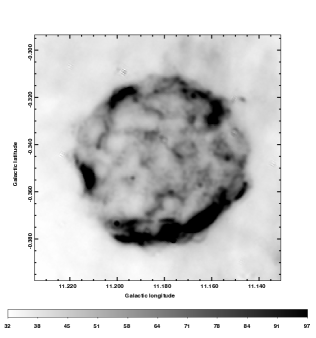
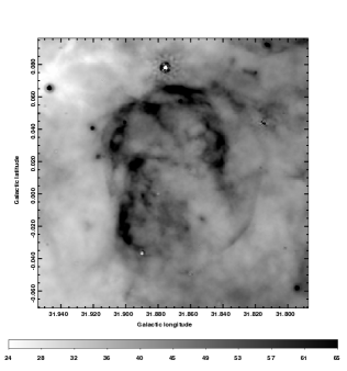
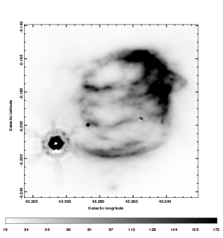
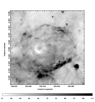
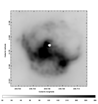
Figure 2.— Examples of level 1 detections at 24 $\micron$. From left to right, top to bottom: G11.2-0.3, G27.4+0.0 (Kes 73), G31.9+0.0 (3C 391), G43.3-0.2 (W49B), G332.4-0.4 (RCW 103) and G349.7-0.2. The greyscale is linear with the ranges in MJy/sr as displayed in the intensity bars below each image. The angular extents of the images differ.

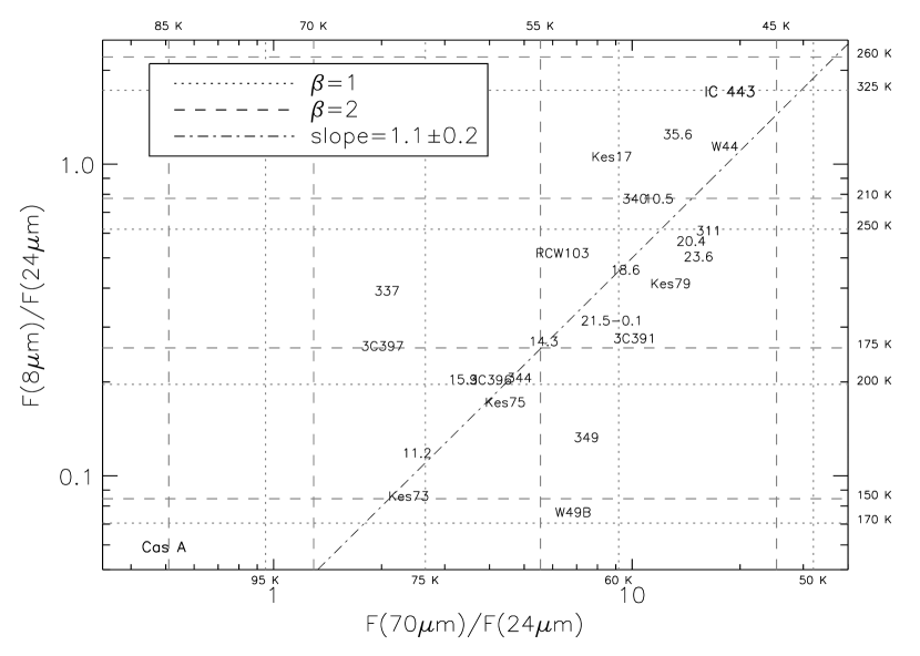
Figure 3.— Color-color plot of the SNRs in our sample detected and measured as a whole. For comparison, we have also plotted the location of Cas A and IC443 in this diagram. We find that this sample is well fitted by a slope of $1.1\pm 0.2$ in this logarithmic representation, showing that 8 and 70 $\micron$ emission are related roughly by a constant while they change dramatically with respect to 24 $\micron$. Vertical lines show the range of expected temperatures for a modified blackbody using only the flux measured at 24 and 70 $\micron$ while for the horizontal lines, the temperatures are calculated using the flux at 8 and 24 $\micron$. Dotted and dashed lines correspond to a $\beta$ of 1 or 2, respectively. If the IR emission at longer wavelengths is mainly due to dust then the range of temperatures for our sample of SNRs is roughly between 50 and 85 K for $\beta$=1 and between 45 and 70 K for $\beta$=2.

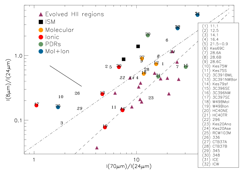
Figure 4.— Color-color plot based on surface brightnesses of localized regions in SNRs in our sample. Ratios for SNRs known to have molecular interactions, atomic fine-structure line emission or PDRs colors are also shown. ICE and ICW refer to IC443, eastern (strong [O I] emission at 63 $\micron$) and western (interacting with a nearby H II region) regions, respectively. Colors of pure infrared synchrotron emission are plotted as a straight line. Color ratios for the diffuse ISM (Compiegne et al., 2010) and evolved H II regions (Paladini et al. (in preparation)) are also included. Remnants with upper flux limits are represented in italic. For comparison, we plot the slope (dotted-dashed line) of $1.1\pm 0.2$ found for the sample of detected remnants and measured as a whole (see Fig. 3). Also depicted is a dashed line showing a different trend for evolved HII regions.

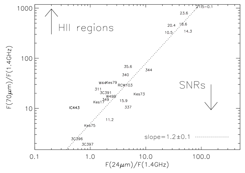
Figure 5.— Ratio of MIPS 70 $\micron$ and radio continuum at 1.4 GHz ($q{{}_{\mathrm{70}}}=\log(F{{}_{\mathrm{70\micron}}}/F{{}_{\mathrm{1.4GHz}}}$)) versus ratio between 24 $\micron$ and radio again ($q{{}_{\mathrm{24}}}$). There is a considerable range in the positions of the SNRs. The ratios are correlated and are well fitted by a slope of 1.2. There seems to exist a group of catalogued sources which have ratios more characteristic of H II regions (upper population in the plot). The infrared counterparts in the lower part of the plot show ratios of infrared (70 $\micron$) to radio comparable to what was found for SNRs in previous studies (e.g., Broadbent et al. (1989)) which suggested ratios of infrared (60 $\micron$) to 2.7 GHz lower than 20. The location of IC443 is also shown. Cas A falls off the plot and below the trend with ratios (0.1, 0.05).

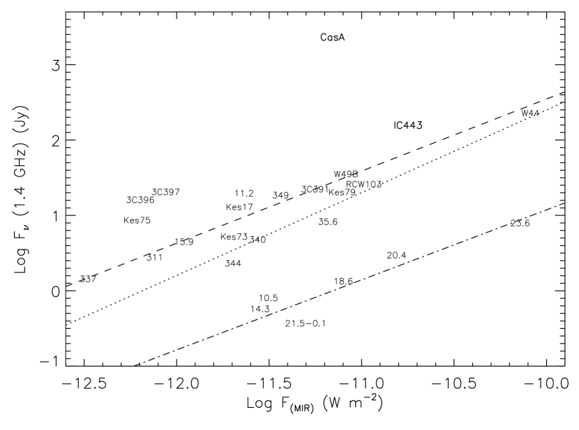
Figure 6.— Correlation between radio and infrared emission. For the entire population, the slope of the correlation is 1.10 (dotted line). There seem to exist two trends. The upper population is more characteristic of SNRs while the lower population looks more like H II regions. The latter are the same objects with the high values of $q{{}_{\mathrm{24}}}$ and $q{{}_{\mathrm{70}}}$ in Figure 5. The slopes for the upper and lower populations are 0.96 (dashed line) and 0.93 (dot-dashed line), respectively, not significantly different. Again, IC443 and Cas A are also included for comparison. Cas A stands out due to its strong radio synchrotron emission.

Figure 7.— SEDs of Chandra SNRs ordered according to approximate remnant’s age (increasing left to right, top to bottom). For the radio, the synchrotron spectrum is shown by the dotted line for the appropriate spectral index, anchored in the observed range at 1 GHz (triangles). The circles indicate the power in the infrared at 8, 24 and 70 $\micron$. In the X-ray, the band (0.3-10 keV) of the Chandra images is used (squares). Horizontal lines represent the width of the bandpass. We also include Cas A and IC443 for comparison. Their infrared flux densities are taken from Hines et al. (2004) and Noriega-Crespo et al. (in preparation) while the X-ray fluxes are from the Chandra Supernova Remnant Catalog and Dwek et al. (1987), respectively. Again, note that for W44 the infrared and X-ray values apply only to the central region while the radio estimate is for the whole remnant. The integrals over the infrared and X-ray range reveal their contributions to cooling the shocked plasma.

Appendix A First Galactic quadrant: 10^∘ $\leq$ l $\leq$ 60^∘

A.1. G10.5-0.0

First reported in Brogan et al. (2006) (hereafter, B06), this remnant was classified as a class II candidate (sources with the highest confidence index of detection are denominated as class I and the least as class III). The remnant has a possible ASCA (Advanced Satellite for Cosmology and Astrophysics) X-ray counterpart (Sugizaki et al., 2001). Figure 8 shows that the 24 $\micron$ emission roughly matches the radio contours. At 70 $\micron$, it only emits in the northern part and at 8 $\micron$, the emission is confused with the background, although an arc of emission close to the X-ray source is well detected. This feature is also present at 24 and 70 $\micron$. There is a small H II region inside the remnant which coincides with some of the 24 $\micron$ emission implying that the flux measurement is an upper bound.

A.2. G11.1+0.1

This is a class I object from B06 with a radio shell morphology. The infrared emission in all wavelengths is easily confused with the background on the southern part of the remnant. However, the brighter radio knots inside the radio contours show strong 24 $\micron$ emission (see Fig. 9).

A.3. G11.2-0.3

This fairly young remnant (1600 yr) contains a millisecond pulsar PSR J1811-1925 at the centre (Kaspi et al., 2001). It is clearly seen in the radio as a circular shell of approximately $4^{\prime}$ diameter (spectral index of 0.6) and it is located at a distance of 4.4 kpc (Green, 2009a, and references therein). Using staring observations with Spitzer, Rho et al. (2009) found Fe emission with temperature and density representative of ejecta material in regions with high Fe content. Koo et al. (2007) detected near-infrared [Fe II] and H₂ filaments within and outside the radio borders of the remnant, respectively. While the H₂ emission is most likely the result of some sort of interaction between the shockwave and the progenitor wind, the [Fe II] emission is thought to be the combination of ejecta and surrounding ISM with a morphology characteristic of an ‘asymmetric explosion’. Recently, new near-infrared spectroscopic observations of dense Fe knots (Moon et al., 2009) strengthened the belief that the SN explosion happened along the north-south direction (in Galactic coordinates). The 24 $\micron$ image (Fig. 10) reveals peaks of mid-infrared emission that coincide morphologically with X-ray emission (Fig. 10). Previously detected in the IRAC wavelengths, this remnant shows 8 $\micron$ emission in the eastern part but since it is diffuse, a clear association is not possible. The same diffuse pattern is seen in the 70 $\micron$ image. Both filaments detected in the southern rim at 8 $\micron$ have correlated emission in the 24 and 70 $\micron$ images, although unresolved. The IRAC colors for these filaments suggest molecular emission from shocked gas (Reach et al., 2006, hereafter, R06). The blob in the most eastern part of the remnant is detected both at 24 and 70 $\micron$ and so it is most likely due to dust.

A.4. G12.5+0.2

This is a possible composite class II remnant from B06. Figure 11 shows a striking ridge of 24 $\micron$ emission on the central-western part of the remnant. To the southwest it borders an IR source. Also, filamentary structure is seen towards the east at the boundary with a dark cloud.

A.5. G14.1+0.1

This is a class II shell remnant from B06. The 24 $\micron$ emission has a horseshoe shape (Fig. 12) which roughly matches the radio morphology. At 8 and 70 $\micron$ only diffuse emission is seen. The remnant is surrounded by all kinds of infrared filaments which without the radio contours would be hard to distinguish from the overall structure.

A.6. G14.3+0.1

This is another class II remnant from B06. While the 8 $\micron$ IRAC image shows emission localized in the eastern part, the 70 $\micron$ emission fills the radio contours uniformly. The 24 $\micron$ emission also fills the contours with two peaks located north and south of the remnant’s centre (see Fig. 13).

A.7. G15.9+0.2

Chandra observations showed that this remnant is young ($\leq 2400$ yr) with an X-ray point source (Reynolds et al., 2006). The obtained X-ray spectrum implied high element abundances characteristic of ejected material. The infrared detections are presented in Figure 14. This remnant was not detected in either the GLIMPSE or IRAS surveys. The 24 $\micron$ emission is bright in the southern-most part. There are also traces of emission in the north rim. At 8 $\micron$, the emission is very faint and mainly seen around the south-eastern radio contours. The 70 $\micron$ image shows diffuse emission extending along the south-eastern part; nevertheless, it is unclear if this is associated with the remnant. Also, in the same area, the remnant seems to be encountering interstellar material, although no maser emission has been reported (Green et al., 1997).

A.8. G16.4-0.5

B06 classified this as a class II partial shell. The 24 $\micron$ emission has a shape similar to a fork with the strongest emission coming from its prongs. The western arc feature does not seem to have a strong counterpart at the other infrared wavelengths, unlike the rest of the structure which shows up diffusely (Fig. 15).

A.9. G18.6-0.2

Another partial shell class II remnant from BG06 is shown in Figure 16. There is a good correspondence between the radio contours and the infrared emission, in particular, for 24 $\micron$. At 70 $\micron$ the strongest infrared emission matches the brightest radio peaks and, at 8 $\micron$, there is diffuse emission which seems to occupy those regions as well, but no clear association can be established based on this filter alone.

A.10. G20.4+0.1

Figure 17 shows a shell class I remnant from B06. The 24 and 70 $\micron$ emission fill the radio contours. The northwestern radio shell is well matched by the 24 and 70 $\micron$ emission and it is surrounded by 8 $\micron$ filaments.

A.11. G21.5-0.9

Tian & Leahy (2008b) suggested that this remnant is at 4.8 Kpc based on HI and CO observations and it has an associated pulsar (PSR J1833-1034) at its centre (Camilo et al., 2006). Figure 18 shows the infrared emission at 24 and 70 $\micron$ associated with the central X-ray contours. There is no distinctive association between the 8 $\micron$ diffuse emission and the Chandra image.

A.12. G21.5-0.1

This is a partial shell remnant identified in BG06, with a possible ASCA X-ray counterpart (Sugizaki et al., 2001). Centred at coordinates $21.6$ and $-0.1$, a ring with $0.5^{\prime}$ radius accounts for most of the 24 $\micron$ emission (Fig. 19). The southern filament which coincides with a bright radio ridge is seen in all of the infrared wavelengths. Below this, there is a filament of 8 $\micron$ immediately outside the radio contours.

A.13. G21.8-0.6 or Kes 69

At a distance of 5.5 Kpc (Tian & Leahy, 2008b), Kes 69 was detected in the GLIMPSE survey and shocked lines are most likely responsible for the majority of the emission seen in the south part of the radio contours (R06). The 8 and 24 $\micron$ images (Fig. 20) show filaments that might be associated with the remnant centre (Kes69C), though there are similar faint structures to the south beyond the radio contours. There is prominent mid-infrared emission north of the remnant due to a bright H II region.

A.14. G23.6+0.3

This remnant has a radio spectral index of -0.34 (Shaver & Goss, 1970). Its odd elongated radio shape is seen to spatially coincide with the 24 $\micron$ emission (Fig. 21). The 8 and 70 $\micron$ emissions are more prominently displaced towards the south and west of the radio boundaries. No maser association has been reported.

A.15. G27.4+0.0 or Kes 73

This remnant has a $4^{\prime}$ diameter shell-like structure in the radio. Tian & Leahy (2008a) reported that this SNR can be as far as 9.8 kpc and be 500-1000 yr old. Vasisht & Gotthelf (1997) discovered a low period (12s) X-ray signal from the central compact source (1E 1841-045). The SNR is not detected at the IRAC wavelengths but it is spectacularly seen at 24 $\micron$ (Fig. 22). This mid-infrared emission traces the X-ray contours extremely well, with both peaking in the northwestern ridge.

A.16. G28.6-0.1

This region is highly contaminated by thermal emission and therefore extremely bright in infrared wavelengths. The three areas chosen to calculate infrared fluxes are identified in Figure 23 by A, B and C. These sources showed a non-thermal spectra in the radio (Helfand et al., 1989) and 20 cm flux densities of 0.73, 1.05 and 1.05 Jy, respectively. The radio morphology of all sources trace closely the 24 $\micron$ shape. Sources B and C do not show any 8 and 70 $\micron$ emission and are only well detected at 24 $\micron$.

A.17. G29.7-0.3 or Kes 75

This composite remnant has an associated pulsar (PSR J1846-0258; Gotthelf et al., 2000) and is thought to have an upper distance limit of 7.5 kpc (Leahy & Tian, 2008). This remnant was not detected in GLIMPSE or IRAS surveys but was well identified using targeted MIPS observations by Morton et al. (2007) where most of the emission at 24 $\micron$ originates from two bright shells located south and west of the remnant’s centre. Figure 24 shows a clear detection at 24 $\micron$ which traces accurately the brighter X-ray regions with the central X-ray peak being the only exception; there is no 8 $\micron$ emission there and the 70 $\micron$ emission appears to be non-existent too. There is also no significant infrared emission at 8 or 70 $\micron$ associated with the bright 24 $\micron$ features. Unrelated 70 $\micron$ emission shows up diffusely in the eastern part of the remnant which overestimates the 70/24 color ratio measured for this region (Kes75S).

A.18. G31.9+0.0 or 3C 391

Green’s SNR catalog describes this object as a shell-type remnant with a spectral index of about 0.49. Previous infrared spectral observations with ISO revealed the existence of ionic lines (Reach & Rho, 2000), in particular [Fe II] at 26 $\micron$ and [S II] at 35 $\micron$ towards the direction of the BML (Broad Molecular Line) region at Galactic coordinates 31.84, 0.03 (Fig. 25). Besides the previous elements, [O IV] at 26 $\micron$ was also detected but found to be 3 times brighter in the radio peak (bar at Galactic coordinates 31.87, 0.06) than in the BML region. Right above this radio peak, the remnant is encountering a nearby molecular cloud (Wilner et al., 1998). All of the above line emitters contaminate the MIPS channels and therefore contribute to fluxes reported in Table 2. Furthermore, Reach et al. (2002) also found clumps of H₂ emission in the BML which was again confirmed with IRAC color ratios by R06. Two 1720 MHz OH masers were detected within the remnant (Frail et al., 1996). IRAC images show emission associated with the western maser where the previously mentioned BML is located. Mid-infrared 24 and 70 $\micron$ emission from MIPSGAL is clearly seen in this region as well (Fig. 25). Previous IRAC observations revealed a rim of [Fe II] emission which matches the brightest radio emission in the north part of the remnant. The same feature is seen in the 24 $\micron$ image which suggests that the bulk of emission at this location can be due to [Fe II] at 26 $\micron$. R06 also found that the infrared emission in the middle knots (east and west at the ‘waist’; the one in the west has the same location as the BML) is produced by shocked molecular gas. These knots are well detected at 24 $\micron$ (with some likely contribution from H₂ S(0) at 28 $\micron$) and are especially strong at 70 $\micron$. The southeastern rim structure (at 24 $\micron$) coincides with an enhancement in the radio and the second maser.

Remnant 3C391 is characterized by a faint outer rim that can be seen both in the radio at 20 cm and in the infrared at 24 $\micron$. This is the collisionless shock where the blast wave encounters the ISM. Although the radio structure is spatially correlated with the faint mid-infrared, a spectral index analysis shows that this 24 $\micron$ emission is too strong to have only a synchrotron origin.

A.19. G33.6+0.1 or Kes 79

This a ‘mixed-morphology’ remnant with a centrally compact X-ray source (Seward et al., 2003). It has an incomplete radio shell of $10^{\prime}$ in size and it is X-ray centre filled. The southern filaments seen in the Chandra image are well detected and have a similar morphology in the 24 $\micron$ image (Fig. 26). Those are located in the same region as a dark cloud, where previous CO and HCO⁺ observations suggested an interplay with a nearby molecular cloud (Green & Dewdney, 1992). These authors also noted that this must be an evolved remnant given its large linear size. Furthermore, using Chandra observations Sun et al. (2004) did not encounter evidence of ejecta material, reinforcing the conclusion that this must be an older remnant (around 6000 yr old). The 24 $\micron$ emission fills and traces the brightest X-ray contours (so called inner-shell) in the central part of the remnant while 8 $\micron$ diffuse emission is present in the northern part of the remnant, but not likely to be associated. Likewise, at 70 $\micron$ it appears that the main contribution to the flux is probably the IRAS source 18501+0038 (represented by a white circle in Fig. 26).

A.20. G34.7-0.4 or W44

This evolved object is classified as a ‘mixed-morphology’ remnant (Rho & Petre, 1998) due to its radio shell with inner X-ray filled emission. It is mainly detected at 70 $\micron$ possibly indicating that it has had time to evolve (see Fig. 27). This is in agreement with the inferred age of about 20000 yr from the characteristic age of the associated pulsar (Wolszczan et al., 1991). In the 70 $\micron$ image, the western filaments trace well the radio contours. In all the infrared wavelengths, there is emission associated to the northern region. This is one of the most stunning detections in GLIMPSE data where R06 found that emission at 4.5 $\micron$ (which is mostly from shocked molecular gas) matches well the radio contours. Previously, Reach et al. (2005b) also detected near-infrared shocked H₂ and millimeter wave molecular lines, which revealed the interaction of the remnant with a GMC. Moreover, the existence of extended maser emission has also been reported (Hewitt et al., 2008) inside of the remnant. Recent Spitzer spectral line analysis (Neufeld et al., 2007) revealed the emission of [Fe II] around 26 $\micron$ and some H₂ at 28 $\micron$ which can be contributors to the faint emission seen in the MIPSGAL 24 $\micron$ image. At 8 $\micron$ the object is easily confused with the diffuse background.

A.21. G35.6-0.4

This object was recently re-classified as a SNR (Green, 2009b). It has a spectral index of 0.47. The radio emission is peaked, with size of $15^{\prime}\times 11^{\prime}$. IRAS emission has not been previously reported. Its emission at 8 and 70 $\micron$ can be more easily confused with the background material and there seems to be no convincing association with the radio contours (Fig. 28). At all wavelengths, there is emission associated with a gamma-ray source HESS 1858+020 and a narrow ridge (jets?) can be seen at 24 $\micron$.

A.22. G39.2-0.3 or 3C396

Several filaments are observed at 24 $\micron$ (Fig. 29). Specifically, the top interior part of the remnant is only observed in this wavelength. Also, recent near-infrared observations (Lee et al., 2009) revealed the presence of [Fe II] and H₂ in the northwestern part of the shell matching the radio emission. The 24 $\micron$ image shows the exact same features which suggests that some emission is probably due to lines in the MIPSGAL band. Other filaments near the centrally projected hot point source (IRAS 19017+0522) are seen at 8, 24 and 70 $\micron$. Previously, R06 had argued that those filaments had colors consistent with PDRs . In that case, the suite of Spitzer passbands is probing the dust emission from PAHs to big grains. The tail of radio emission mentioned in Patnaik et al. (1990) is partially traced by 24 and 70 $\micron$ with some spatial mismatch. There is a bright filament in the south part of this tail, which is detected in all of the infrared wavelengths. Moreover, in the eastern part of the tail, a filament of infrared emission also seems to match exactly the radio contour. The infrared emission that is in between the tail and the remnant is most likely to be caused by thermal dust grains.

A.23. G41.1-0.3 or 3C 397

This is another shell-type morphology remnant with spectral index of 0.48 (Green, 2009a). Its uncommon rectangular shape on the upper edge suggests interaction with the ISM, specifically a dense molecular cloud inferred through CO observations (Safi-Harb et al., 2005). Based on Chandra data, the same authors propose that the remnant is about 5300 yr old and is now starting the radiative stage. The 8 and 70 $\micron$ images show some emission in the north part of the remnant (Fig. 30). The 24 $\micron$ image reveals rich filamentary structure that nicely resembles the entire X-ray counterpart. The GLIMPSE survey reported a faint detection in regions where IRAC colors suggested shocked emission from ionic lines (R06).

A.24. G43.3-0.2 or W49B

W49B is characterized by an odd ‘barrel’-shaped morphology in the radio (Moffett & Reynolds, 1994). R06 reported that most of the emission at the IRAC wavelengths is consistent with shocked ionic and molecular emission lines. Later on, near-infrared observations revealed that the [Fe II] morphology, at 1.64 $\micron$, is similar to the radio structure and the 2.12 $\micron$ H₂ can be found primarily in the south (right below the [Fe II] ridge) and in the northwestern part of the remnant (Keohane et al., 2007). With the help of Chandra data, these authors also reported an overabundance of heavy elements thus suggesting that the X-ray emission is dominated by the ejected material as found previously by Hwang et al. (2000) using ASCA data. Both MIPS channels (see Fig. 31) show interesting filamentary structure and are brighter in the same locations, thus indicating that there is a strong dust continuum contribution as the primary emission mechanism in the far-infrared. However, note that the 24 $\micron$ image seems to trace well the ionic shocked component within the X-ray contours.

A.25. G54.4-0.3

GLIMPSE data (R06) revealed two regions with the same color ratios as photodissociation regions whose infrared filaments spatially match the radio profile. Those are also seen as filaments in the 24 $\micron$ and diffuse emission at 70 $\micron$ (see Fig. 32). Fluxes for those two regions are reported in Table 2.

Appendix B Fourth Galactic quadrant: 295^∘$\leq$l$\leq$350^∘

B.1. G296.8-0.3

This remnant with an elongated radio shell is at 9.6 kpc and has an age between $(2-10)\times 10^{3}$ yr (Gaensler et al., 1998). These authors also concluded that its radio morphology might have been shaped either due to mass loss from winds or interaction with the ISM. There is an arc of bright 24 $\micron$ emission which matches the strongest radio synchrotron emission in the northwest region. No IRAS or GLIMPSE detection has been reported. As seen in Fig. 33, there is some diffuse 70 $\micron$ emission around it that is unlikely to be associated with the remnant.

B.2. G304.6+0.1 or Kes 17

Infrared emission from the northwestern part was detected in the GLIMPSE data and attributed to shocked molecular gas (R06). Those filaments are also present in the 24 $\micron$ image (Fig. 34). Moreover, at that same wavelength, there is emission along the south which spatially coincides with the radio ridge. At 70 $\micron$, there is just filled emission around the northwestern shell.

B.3. G310.8-0.4 or Kes 20A

MOST observations show a well-defined eastern radio shell with a weak western counterpart (Whiteoak & Green, 1996). Diffuse thermal emission in the western counterpart of the remnant has led to previous confusion regarding the thermal or non-thermal origin of this SNR. Following the radio contours to the south west of the bright compact eastern radio peak is an arc of 24 $\micron$ emission (Fig. 35). This feature is also present at 70 $\micron$ but it is not clearly distinguishable at 8 $\micron$. There are also filaments of diffuse infrared emission that follow the north-south eastern radio shell.

B.4. G311.5-0.3

Whiteoak & Green (1996) first identified this as a shell type SNR. With GLIMPSE data, R06 detected an incomplete shell (brightest in the western part). Color-color ratios led to the conclusion that infrared emission was due to shocked molecular gas. Both MIPS images show the same approximate morphology following a circular shell (Fig. 36).

B.5. G332.4-0.4 or RCW 103

This young remnant (age about 2000 yr) has a shell-like radio morphology and is at a distance of 3.1 kpc (Green, 2009a and references herein). It has a soft X-ray point source near the centre of the remnant (Tuohy & Garmire, 1980). The 24 $\micron$ image (Fig. 37) shows extensive diffuse and filamentary emission related to the remnant, spatially correlated with the radio. Numerous small filaments trace the outer borders of the synchrotron emission. There is a dark arc in the centre left of the remnant where the IR and X-ray shells seem to be incomplete. For the southern bright rim, R06 found colors indicating shocked molecular gas along with some ionic emission, which corroborated the reported detection of ionized species by Oliva et al. (1999b). Around 24 $\micron$, the ISO spectrum showed strong emission mainly from [Fe II] as well as [O IV]. These authors also reported that heavy elements are in the gas phase given their solar-like abundances and therefore most of the infrared emission in that rim must be the result of fine-structure lines. The 24 $\micron$ morphology is very similar to the X-ray emission, as seen in other young remnants.

B.6. G336.7+0.5

There is an arc in the 24 $\micron$ image which matches roughly a radio counterpart emission peak (see Fig. 38). At 8 and 70 $\micron$, there is some diffuse emission in the south which coincides with a brighter radio region but it seems unlikely that they are associated. The flattened indented outer radio contours to the south west coincide with with a dark cloud, possibly the locus of interaction of the SNR with the ISM.

B.7. G337.2-0.7

The radio contours from MOST observations indicate that this is a compact circular shell remnant (Whiteoak & Green, 1996). It has not been detected in the IRAC bands or IRAS surveys. The remnant is more complex in the X-ray and mid-infrared (Fig. 39), with the 24 $\micron$ emission composed of several filaments forming two distorted apparent shells. The interior one is almost complete and is located in the western part. The other is visible as two long filaments mainly in the north-south direction in the eastern part of the remnant. Both relate closely to the contours of the Chandra X-ray emission. There is some 70 $\micron$ diffuse emission in the north-eastern part but unlikely to be related with the remnant.

B.8. G340.6+0.3

This is a circular shell remnant in the radio located at 15 kpc (Kothes & Dougherty, 2007). Filaments of 24 $\micron$ emission follow the radio contours especially in the south west (see Fig. 40). Also, emission from two projected IRAS point sources, 16441-4427 and 16441-4429, situated in the north region of the SNR at opposing sides, enhance the flux considerably at the MIPSGAL wavelengths; note that in the Spitzer bands there is considerable extended emission at these peaks.

B.9. G344.7-0.1

Dubner et al. (1993) reported an angular size of 33 pc in the radio which agrees with the estimate of a middle-aged remant as based on the X-ray plasma temperature found using ASCA data Yamauchi et al. (2005). Figure 41 shows that the emission at all three infrared wavelengths is brightest at the central radio peak. Previous GLIMPSE analysis showed that this structure had colors consistent with shocked ionized gas (R06). Although now clearly diffuse emission, this peak was catalogued as IRAS 17003-4136. The 24 $\micron$ image also shows a few striking filaments associated with the outer radio boundaries, especially where compressed at the northwest.

B.10. G345.7-0.2

A rim of emission at 24 and 70 $\micron$ is detected in the south-eastern part of the remnant (Fig. 42), possibly shocked dust from interaction with the adjacent dark cloud. No maser association is reported (Green et al., 1997).

B.11. G348.5-0.0

This SNR is independent from G348.5+0.1 (see below), although its radio morphology looks like a jet of material emanating from CTB 37A (Kassim et al., 1991). GLIMPSE data revealed that the arc of associated infrared emission is mainly dominated by ionic shocks (R06). Figure 43 shows the same structure at 24 and 70 $\micron$, the 24 $\micron$ emission being the strongest of all.

B.12. G348.5+0.1 or CTB 37A

GLIMPSE analysis supports the idea that this remnant is interacting with dense interstellar gas, first indicated by the presence of masers (Frail et al., 1996) within the remnant. Reynoso & Mangum (2000) found CO clouds at approximately the same velocities and locations of the OH 1720 MHz masers. Figure 43 shows that the MIPSGAL images have the same diffuse emission seen at the IRAC wavelengths including the eastern patch of infrared emission which is thought to be physically associated with a maser (and whose IRAC colors suggest emission from shocked molecular gas as noted by R06). At 24 $\micron$ there are also southern filaments which closely trace the radio boundaries. Bright infrared emission on the northwest fills the faint radio emission part of the remnant and its IRAC colors are similar to photodissociation regions (R06).

B.13. G348.7+0.3 or CTB 37B

In this very confused field, Figure 44 shows that the radio peak from MOST contours has an associated mid-infrared peak at 24 $\micron$. In addition there are some filaments within the remnant that seem to be the result of interaction with the ISM. Chandra follow-up observations of a Gamma-ray source (HESS J1713-381) thought to be associated with CTB 37B (Aharonian et al., 2008 and references therein) also detected X-ray thermal emission close to the remnant centre whose temperature suggested a middle-aged SNR (about 5000 yr).

B.14. G349.7+0.2

OH maser emission was found in the remnant’s interior by Frail et al. (1996) and evidence of interaction with a molecular cloud was later strengthened by Reynoso & Mangum (2001) with CO observations. With extremely similar X-ray and radio morphology, its corresponding brightness in both regimes is also high (Lazendic et al., 2005). The infrared emission is present with a similar morphology at all three wavelengths (Fig. 45). The infrared is strongly peaked within the X-ray contours, but not closely related, except for the 24 $\micron$ emission. Previous GLIMPSE analysis showed infrared emission in all of the IRAC bands (R06).

Appendix C Individual Images

Images of the infrared emission for each detected remnant follow. The order is the same for all the figures and consists of the black and white 24 $\micron$ image (colorbar in units of MJy/sr) on the left and the 3-color image on the right, with 8, 24 and 70 $\micron$ being blue, green and red, respectively. Overlaid in each image are contours either from radio or X-ray observations when available (see §2.2). Images are all in Galactic coordinates, and our remarks on north (up), east (left), etc., are with respect to this system. Also indicated is the angular scale which can be compared with the few arcminute resolution of IRAS.

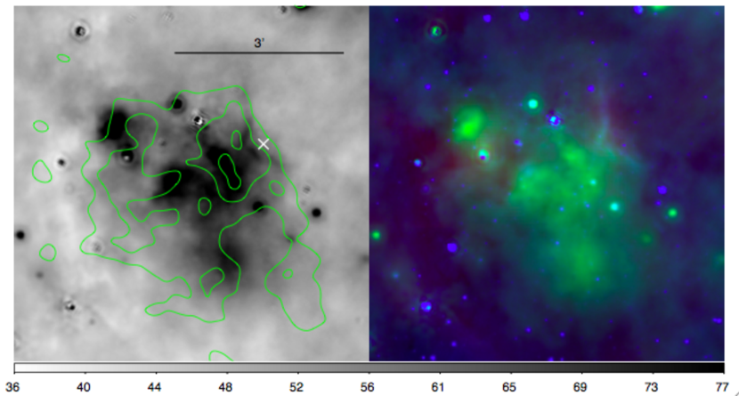
Figure 8.— SNR G10.5-0.0. Contours from VLA 20 cm observations: levels are 13, 17, 21 and 24 mJy/beam. The cross represents the location of the associated X-ray source (AX J180902-1948).

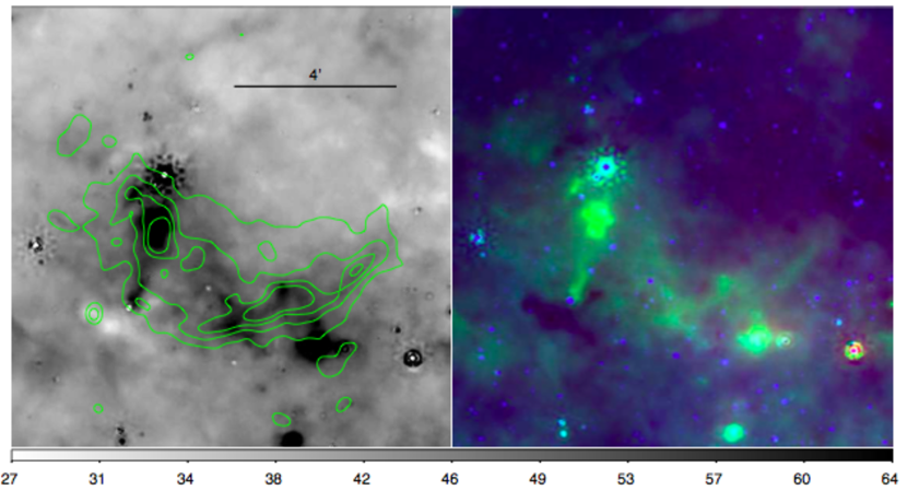
Figure 9.— SNR G11.1+0.1. Contours from VLA 20 cm observations: levels are 14, 18, 22 and 26 mJy/beam.

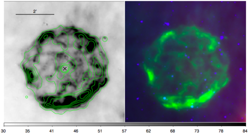
Figure 10.— SNR G11.2-0.3. Contours from Chandra observations: levels are 2, 6, 9, 13, $16\times 10^{-7}$ photons/cm²/sec/pixel. The cross marks the location of the associated pulsar (AX J1811.5-1926).

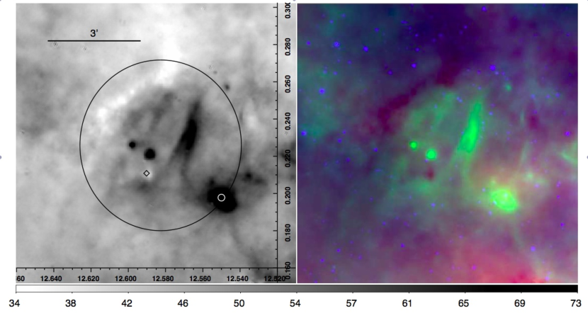
Figure 11.— SNR G12.5+0.2. Positions of a maser (diamond) and nearby infrared IRAS (circle) source are overlaid. Also shown is a circle showing the approximate size and location of the remnant in the radio as seen in Fig.2 from B06.

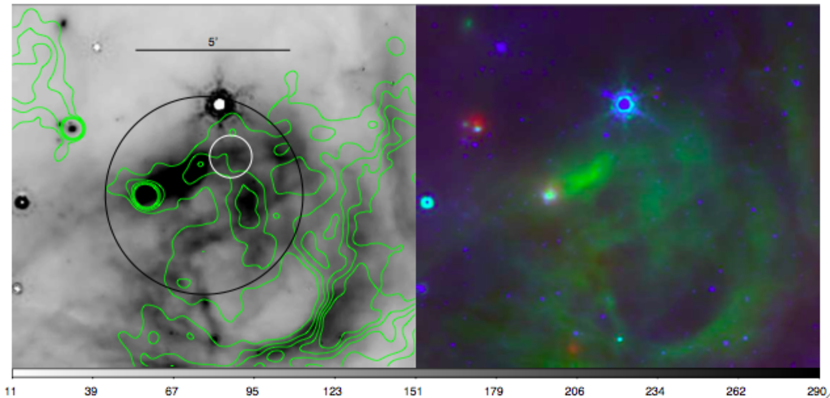
Figure 12.— SNR G14.1-0.1.Contours from VLA 20 cm observations: levels are 18.5 to 28, in steps of 2.4 mJy/beam. The bigger circle (in white) marks the approximate location of the remnant within the confused region (Fig.2 from B06); and the smaller circle (in black) indicates the area used to infer color ratios.

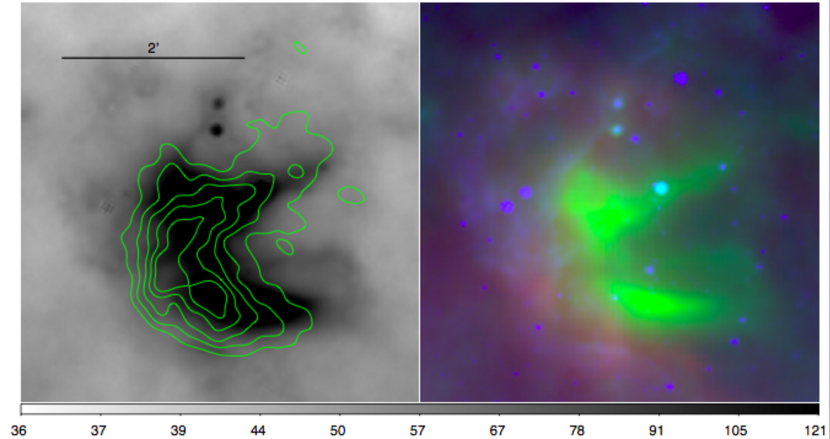
Figure 13.— SNR G14.3+0.1. Contours from VLA 20 cm observations: levels are 16, 20, 24 and 28 mJy/beam.

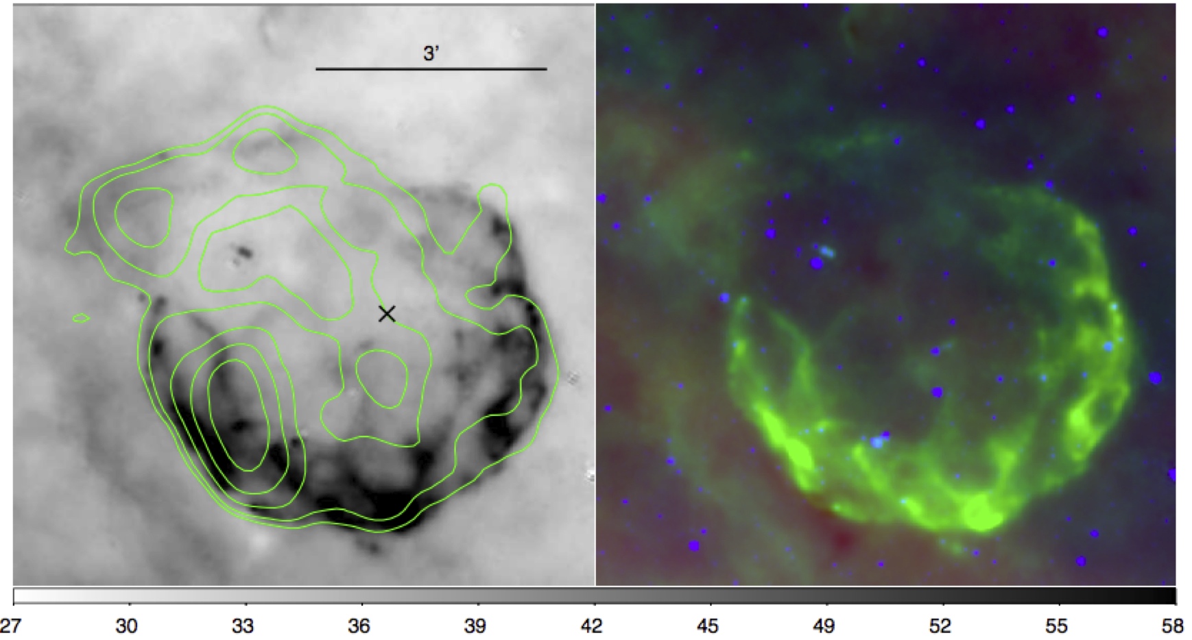
Figure 14.— SNR G15.9+0.2. Contours from VLA 20 cm observations: levels are 0.05, 0.12, 0.34, 0.7 and 1.2 Jy/beam. The cross marks the location of an X-ray source (CXOU J181852.0-150213)

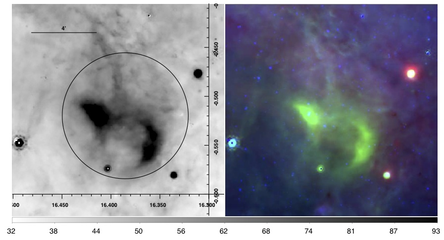
Figure 15.— SNR G16.4-0.5. Also shown is a circle (in black) which marks the approximate location of the remnant in the radio as seen in Fig.2 from B06.

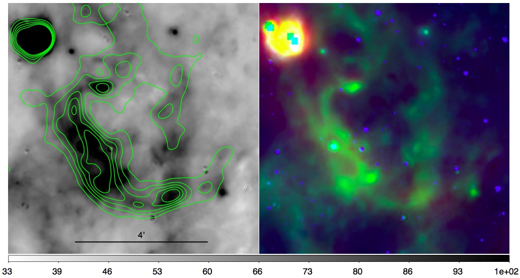
Figure 16.— SNR G18.6-0.2. Contours from VLA 20 cm observations: levels are from 18 to 30, in steps of 4 mJy/beam.

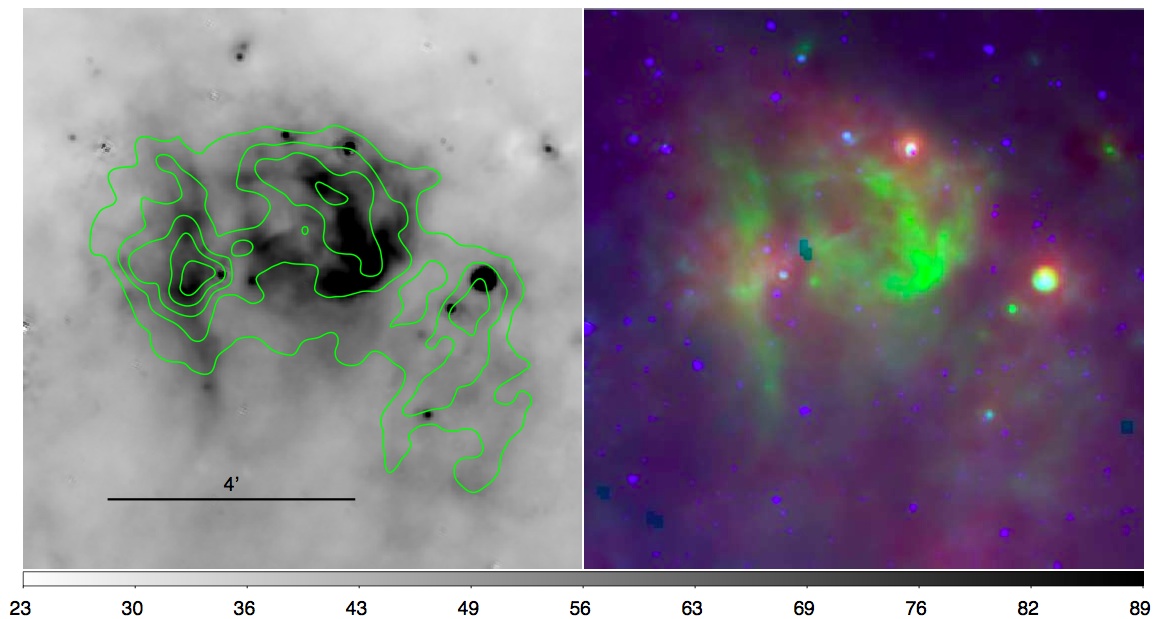
Figure 17.— SNR G20.4+0.1. Countours from VLA 20 cm observations: levels are from 10 to 20, in steps of 2.5 mJy/beam.

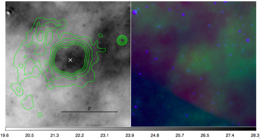
Figure 18.— SNR G21.5-0.9. Contours from Chandra observations: levels are 2, 3, 6.5, 12 and $20\times 10^{-7}$ photons/cm²/sec/pixel. The cross locates PSR J1833-1034.

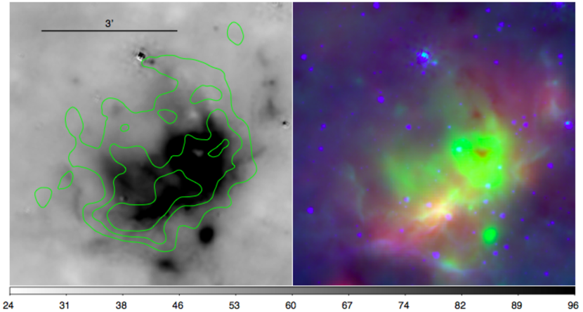
Figure 19.— SNR G21.5-0.1. Contours from VLA 20 cm observations: levels are from 7 to 10, in steps of 1 mJy/beam.

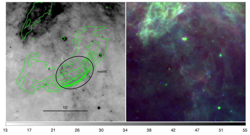
Figure 20.— SNR G21.8-0.6. Contours from VLA 20 cm observations: levels are from 20 to 100, in steps of 20 mJy/beam. Region used for partial photometry is also indicated in the figure (in black)

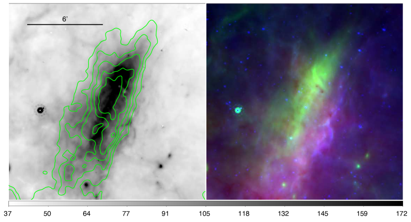
Figure 21.— SNR G23.6+0.3. Contours from VLA 20 cm observations: levels are from 10 to 22, in steps of 3 mJy/beam.

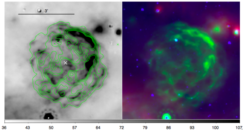
Figure 22.— SNR G27.4+0.0. Contours from Chandra observations: levels are from 2 to $10\times 10^{-7}$, in steps of $2\times 10^{-7}$ photons/cm²/sec/pixel. The cross represents the location of the central X-ray source AX J1841.3-0455.

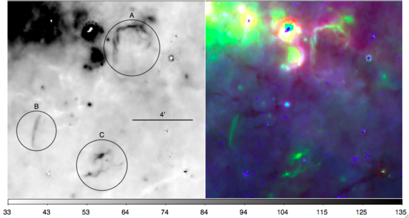
Figure 23.— Vicinity of SNR G28.6+0.1. Regions A, B and C are known to have non-thermal radio emission (Helfand et al., 1989) and represent the regions used to estimate color ratios.

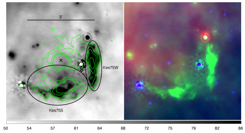
Figure 24.— SNR G29.7-0.3. Contours from Chandra observations: levels are 1.3, 1.8, 3.2, 5.5 and $8.7\times 10^{-7}$ photons/cm²/sec/pixel. The cross marks the location of the pulsar AX J1846.4-0258. Regions used for partial photometry are also indicated in the figure (in black).

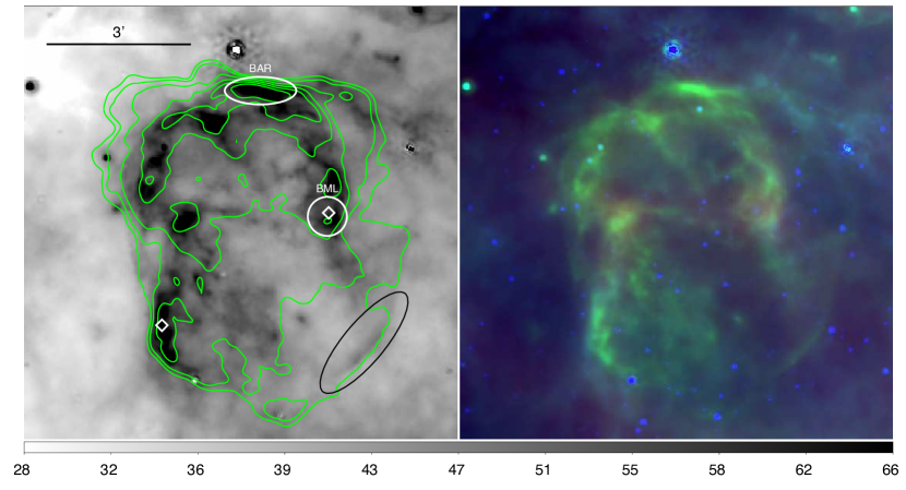
Figure 25.— SNR G31.9+0.0. Contours from VLA 20 cm observations: levels are 15, 28, 69, 140, 230 and 350 mJy/beam. The two maser locations are represented by diamonds. The ellipse (in black) in the southwestern part of the remnant locates a portion of the possible collisionless shock. Regions used for partial photometry are also indicated in the figure (in white).

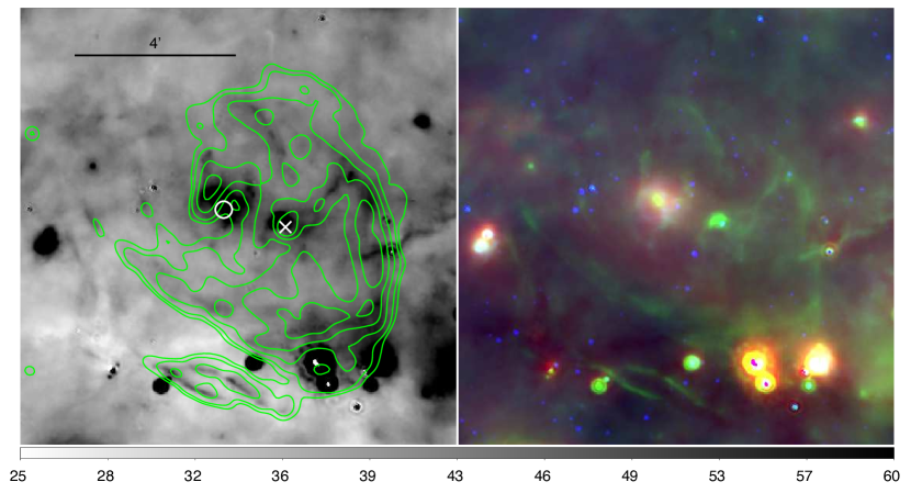
Figure 26.— SNR G33.6+0.1. Contours from Chandra observations: levels are 1.5, 2, 3.6, 6.3 and $10\times 10^{-7}$ photons/cm²/sec/pixel. The cross marks the location of PSR J1852+0040 and the circle represents an IRAS point source.

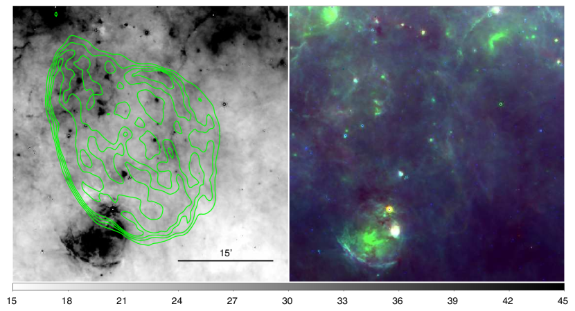
Figure 27.— SNR G34.7-0.4. Contours from VGPS 21 cm observations: levels are 35, 52, 68 and 85 Jy/beam.

Figure 28.— SNR G35.6-0.4. Contours from VGPS 21 cm observations: levels are from 18 to 30, in steps of 3 Jy/beam. The cross marks the location of $\gamma$-ray source J1858+020.

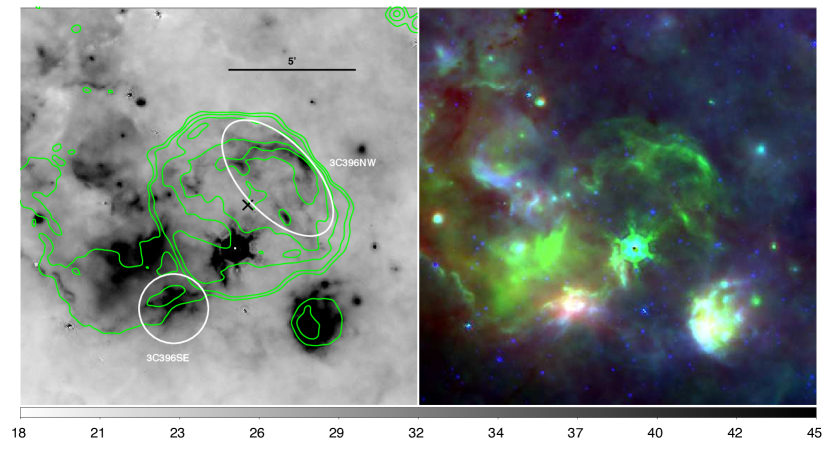
Figure 29.— SNR G39.2-0.3. Contours from 20cm VLA observations: levels are 1, 4, 12, 26 and 45 mJy/beam. The cross represents the location of the X-ray source J190406.5+052646. Regions used for partial photometry are also indicated in the figure (in white).

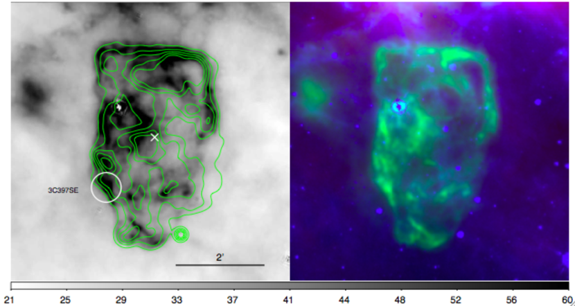
Figure 30.— SNR G41.1-0.3. Contours from Chandra observations: levels are 2, 4.3, 6.5, 8.8 and $11\times 10^{-7}$ photons/cm²/sec/pixel. The cross represents the location of the X-ray source J1907.5+0708. Region used for partial photometry is also indicated in the figure (in white).

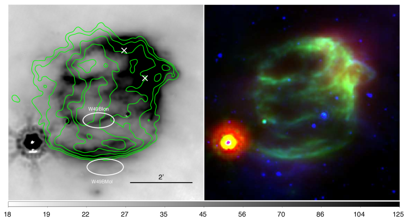
Figure 31.— SNR G43.3-0.2. Contours from Chandra observations: levels are 2, 3.1, 6.5, 12 and $20\times 10^{-7}$ photons/cm²/sec/pixel. The crosses represent the location of the X-ray source J1911.0+0906 and $\gamma$-ray source J1911.0+0905. Regions used for partial photometry are also indicated in the figure (in white).

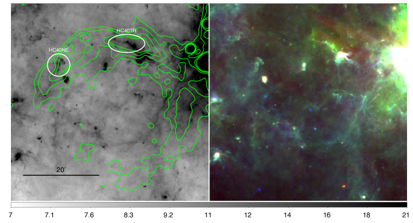
Figure 32.— SNR G54.4-0.3. Contours from VGPS 21 cm observations: levels are from 9.5 to 14, in steps of 1.5 Jy/beam. Regions used for partial photometry are also indicated in the figure (in white).

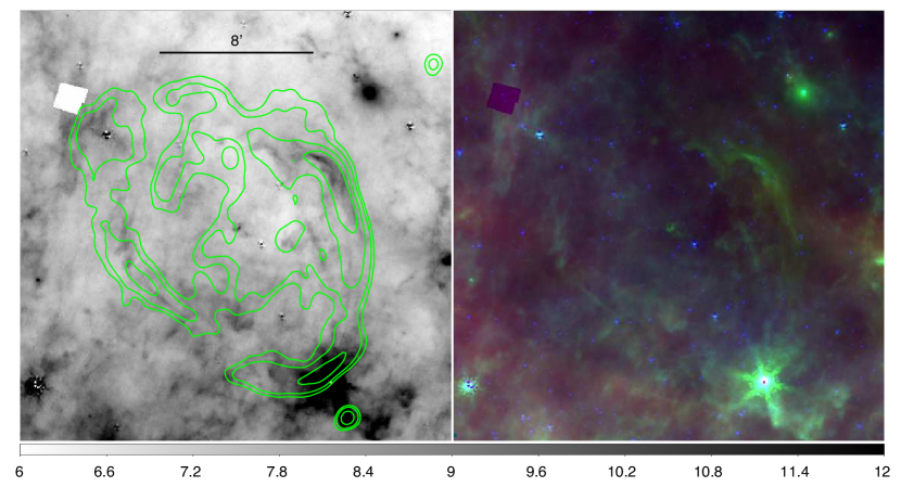
Figure 33.— SNR G296.8-0.3. Contours from MOST observations: levels are 10, 22, 58, 120 and 200 mJy/beam.

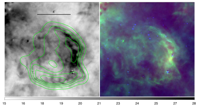
Figure 34.— SNR G304.6+0.1. Contours from MOST observations: levels are 0.06 to 0.5, in steps of 0.11 Jy/beam.

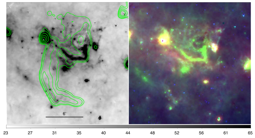
Figure 35.— SNR G310.8-0.4. Contours from MOST observations: levels are 35, 58, 126, 240 and 400 mJy/beam.

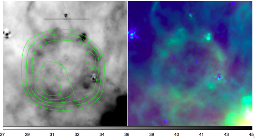
Figure 36.— SNR G311.5-0.3. Contours from MOST observations: levels are 0.1, 0.14, 0.18, 0.24 and 0.27 Jy/beam.

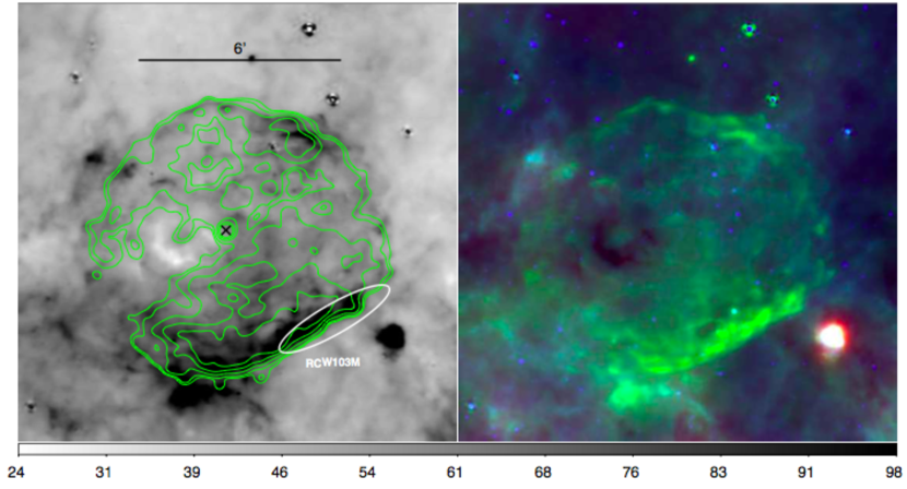
Figure 37.— SNR G332.4-0.4. Contours from Chandra observations: levels are 0.8, 1.1, 2, 3.4 and $5.5\times 10^{-6}$ photons/cm²/sec/pixel. The cross shows the location of the X-ray source 2E 1613.5-5053. Region used for partial photometry is also indicated in the figure (in white).

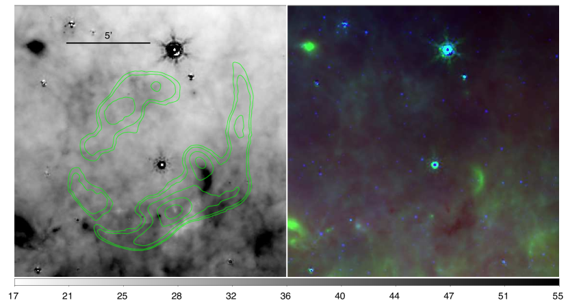
Figure 38.— SNR G336.7+0.5. Contours from MOST observations: levels are 35, 45, 76, 130 and 200 mJy/beam.

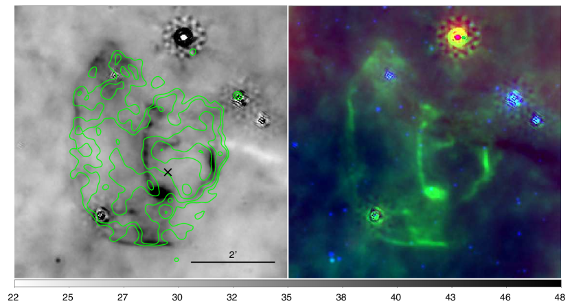
Figure 39.— SNR G337.2-0.7. Contours from Chandra observations: levels are 0.8, 1, 1.6, 2.6 and $4\times 10^{-7}$ photons/cm²/sec/pixel. The cross shows the location of the X-ray source J163931.4-475019.

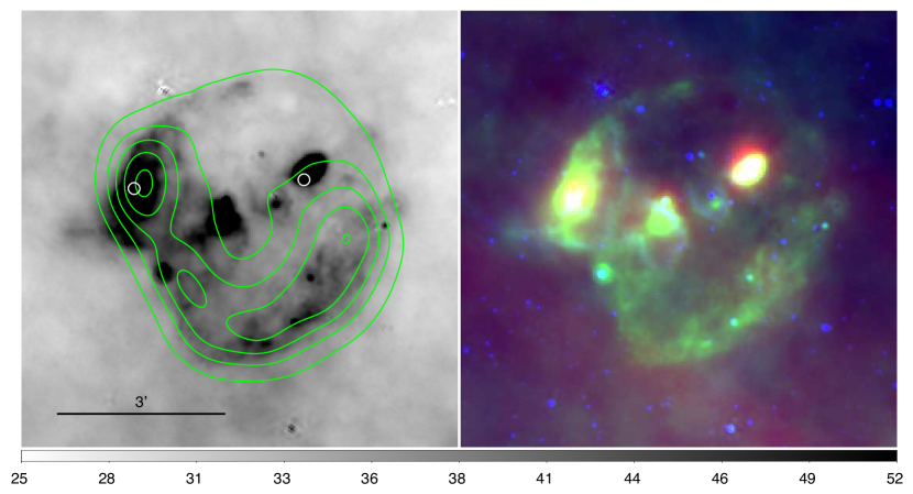
Figure 40.— SNR G340.6-0.3. Contours from MOST observations: levels are from 50 to 350, in steps of 75 mJy/beam. Circles represent the location of two IRAS point sources.

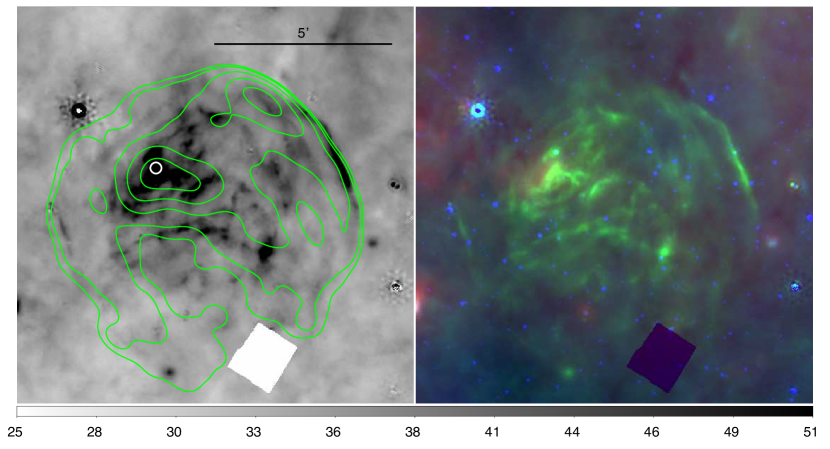
Figure 41.— SNR G344.7-0.1. Contours from MOST observations: levels are 16, 21, 35, 58 and 90 mJy/beam. Circle represents the location of a catalogued IRAS point source corresponding to the diffuse emission peak.

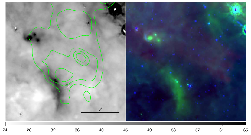
Figure 42.— SNR G345.7-0.2. Contours from MOST observations: levels are from 10 to 40, in steps of 10 mJy/beam. PSR B1703-40 is located at brightest radio peak.

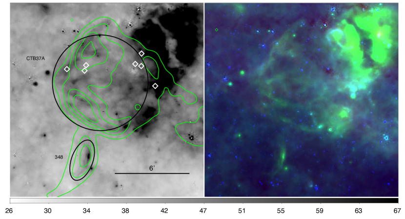
Figure 43.— SNR G348.5-0.0 (south-central countours) and the larger SNR G348.5+0.1. Contours from MOST observations: levels are 0.3, 0.7, 1.1, 1.6 and 2 Jy/beam. Diamonds represent maser locations. Regions used for partial photometry are also indicated in the figure (in black).

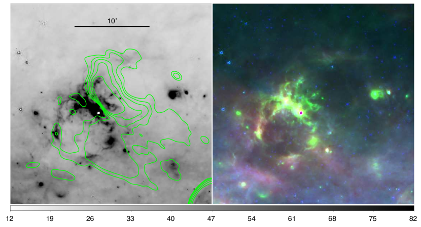
Figure 44.— SNR G348.7+0.3. Contours from MOST observations: levels are 0.03, 0.08, 0.16, 0.32 and 0.55 Jy/beam.

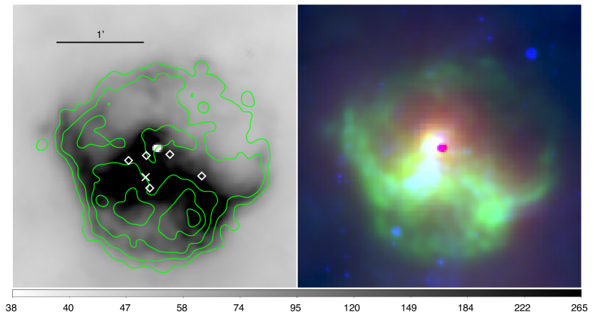
Figure 45.— SNR G349.7-0.2. Contours from Chandra observations: levels are 0.3, 0.7, 1.9, 3.8, 6.5 and $10\times 10^{-7}$ photons/cm²/sec/pixel. Masers are represented by diamonds and the cross marks the location of X-ray source J171801.0-372617.

References

- Aharonian et al. (2008) Aharonian, F., Akhperjanian, A. G., Barres de Almeida, U., Bazer-Bachi, A. R., Behera, B., Beilicke, M., Benbow, W., Bernlöhr, K., Boisson, C., Borrel, V., Braun, I., Brion, E., Brucker, J., Bühler, R., Bulik, T., Büsching, I., Boutelier, T., Carrigan, S., Chadwick, P. M., Chaves, R. C. G., Chounet, L., Clapson, A. C., Coignet, G., Cornils, R., Costamante, L., Dalton, M., Degrange, B., Dickinson, H. J., Djannati-Ataï, A., Domainko, W., O’C. Drury, L., Dubois, F., Dubus, G., Dyks, J., Egberts, K., Emmanoulopoulos, D., Espigat, P., Farnier, C., Feinstein, F., Fiasson, A., Förster, A., Fontaine, G., Funk, S., Füßling, M., Gabici, S., Gallant, Y. A., Giebels, B., Glicenstein, J. F., Glück, B., Goret, P., Hadjichristidis, C., Hauser, D., Hauser, M., Heinzelmann, G., Henri, G., Hermann, G., Hinton, J. A., Hoffmann, A., Hofmann, W., Holleran, M., Hoppe, S., Horns, D., Jacholkowska, A., de Jager, O. C., Jung, I., Katarzyński, K., Kaufmann, S., Kendziorra, E., Kerschhaggl, M., Khangulyan, D., Khélifi, B., Keogh, D., Komin, N., Kosack, K., Lamanna, G., Latham, I. J., Lemoine-Goumard, M., Lenain, J., Lohse, T., Martin, J. M., Martineau-Huynh, O., Marcowith, A., Masterson, C., Maurin, D., McComb, T. J. L., Moderski, R., Moulin, E., Naumann-Godo, M., de Naurois, M., Nedbal, D., Nekrassov, D., Nolan, S. J., Ohm, S., Olive, J., de Oña Wilhelmi, E., Orford, K. J., Osborne, J. L., Ostrowski, M., Panter, M., Pedaletti, G., Pelletier, G., Petrucci, P., Pita, S., Pühlhofer, G., Punch, M., Quirrenbach, A., Raubenheimer, B. C., Raue, M., Rayner, S. M., Renaud, M., Rieger, F., Reimer, O., Ripken, J., Rob, L., Rosier-Lees, S., Rowell, G., Rudak, B., Ruppel, J., Sahakian, V., Santangelo, A., Schlickeiser, R., Schöck, F. M., Schröder, R., Schwanke, U., Schwarzburg, S., Schwemmer, S., Shalchi, A., Skilton, J. L., Sol, H., Spangler, D., Stawarz, Ł., Steenkamp, R., Stegmann, C., Superina, G., Tam, P. H., Tavernet, J., Terrier, R., van Eldik, C., Vasileiadis, G., Venter, C., Vialle, J. P., Vincent, P., Vivier, M., Völk, H. J., Volpe, F., Wagner, S. J., Ward, M., Zdziarski, A. A., & Zech, A. 2008, A&A, 486, 829
- Appleton et al. (2004) Appleton, P. N., Fadda, D. T., Marleau, F. R., Frayer, D. T., Helou, G., Condon, J. J., Choi, P. I., Yan, L., Lacy, M., Wilson, G., Armus, L., Chapman, S. C., Fang, F., Heinrichson, I., Im, M., Jannuzi, B. T., Storrie-Lombardi, L. J., Shupe, D., Soifer, B. T., Squires, G., & Teplitz, H. I. 2004, ApJS, 154, 147
- Arendt (1989) Arendt, R. G. 1989, ApJS, 70, 181
- Arendt et al. (1999) Arendt, R. G., Dwek, E., & Moseley, S. H. 1999, ApJ, 521, 234
- Barlow et al. (2010) Barlow, M. J., Krause, O., Swinyard, B. M., Sibthorpe, B., Besel, M., Wesson, R., Ivison, R. J., Dunne, L., Gear, W. K., Gomez, H. L., Hargrave, P. C., Henning, T., Leeks, S. J., Lim, T. L., Olofsson, G., & Polehampton, E. T. 2010, A&A, 518, L138+
- Bell (2003) Bell, E. F. 2003, ApJ, 586, 794
- Benjamin et al. (2003) Benjamin, R. A., Churchwell, E., Babler, B. L., Bania, T. M., Clemens, D. P., Cohen, M., Dickey, J. M., Indebetouw, R., Jackson, J. M., Kobulnicky, H. A., Lazarian, A., Marston, A. P., Mathis, J. S., Meade, M. R., Seager, S., Stolovy, S. R., Watson, C., Whitney, B. A., Wolff, M. J., & Wolfire, M. G. 2003, PASP, 115, 953
- Blair et al. (2007) Blair, W. P., Ghavamian, P., Long, K. S., Williams, B. J., Borkowski, K. J., Reynolds, S. P., & Sankrit, R. 2007, ApJ, 662, 998
- Borkowski et al. (2006) Borkowski, K. J., Williams, B. J., Reynolds, S. P., Blair, W. P., Ghavamian, P., Sankrit, R., Hendrick, S. P., Long, K. S., Raymond, J. C., Smith, R. C., Points, S., & Winkler, P. F. 2006, ApJ, 642, L141
- Boyle et al. (2007) Boyle, B. J., Cornwell, T. J., Middelberg, E., Norris, R. P., Appleton, P. N., & Smail, I. 2007, MNRAS, 376, 1182
- Broadbent et al. (1989) Broadbent, A., Osborne, J. L., & Haslam, C. G. T. 1989, MNRAS, 237, 381
- Brogan et al. (2006) Brogan, C. L., Gelfand, J. D., Gaensler, B. M., Kassim, N. E., & Lazio, T. J. W. 2006, ApJ, 639, L25
- Camilo et al. (2006) Camilo, F., Ransom, S. M., Gaensler, B. M., Slane, P. O., Lorimer, D. R., Reynolds, J., Manchester, R. N., & Murray, S. S. 2006, ApJ, 637, 456
- Carey et al. (2009) Carey, S. J., Noriega-Crespo, A., Mizuno, D. R., Shenoy, S., Paladini, R., Kraemer, K. E., Price, S. D., Flagey, N., Ryan, E., Ingalls, J. G., Kuchar, T. A., Pinheiro Gonçalves, D., Indebetouw, R., Billot, N., Marleau, F. R., Padgett, D. L., Rebull, L. M., Bressert, E., Ali, B., Molinari, S., Martin, P. G., Berriman, G. B., Boulanger, F., Latter, W. B., Miville-Deschenes, M. A., Shipman, R., & Testi, L. 2009, PASP, 121, 76
- Carter et al. (1997) Carter, L. M., Dickel, J. R., & Bomans, D. J. 1997, PASP, 109, 990
- Cesarsky et al. (1999) Cesarsky, D., Cox, P., Pineau des Forêts, G., van Dishoeck, E. F., Boulanger, F., & Wright, C. M. 1999, A&A, 348, 945
- Chen et al. (2004) Chen, Y., Su, Y., Slane, P. O., & Wang, Q. D. 2004, ApJ, 616, 885
- Churchwell et al. (2009) Churchwell, E., Babler, B. L., Meade, M. R., Whitney, B. A., Benjamin, R., Indebetouw, R., Cyganowski, C., Robitaille, T. P., Povich, M., Watson, C., & Bracker, S. 2009, PASP, 121, 213
- Clark & Stephenson (1977) Clark, D. H. & Stephenson, F. R. 1977, The historical supernovae, ed. Clark, D. H. & Stephenson, F. R.
- Compiegne et al. (2010) Compiegne, M., Flagey, N., Noriega-Crespo, A., Martin, P. G., Bernard, J., Paladini, R., & Molinari, S. 2010, ArXiv e-prints
- Compiègne et al. (2010) Compiègne, M., Flagey, N., Noriega-Crespo, A., Martin, P. G., Bernard, J., Paladini, R., & Molinari, S. 2010, ApJ, 724, L44
- Douvion et al. (2001) Douvion, T., Lagage, P. O., Cesarsky, C. J., & Dwek, E. 2001, A&A, 373, 281
- Draine (1981) Draine, B. T. 1981, ApJ, 245, 880
- Draine (2003) —. 2003, ARA&A, 41, 241
- Dubner et al. (1993) Dubner, G. M., Moffett, D. A., Goss, W. M., & Winkler, P. F. 1993, AJ, 105, 2251
- Dwek (1987) Dwek, E. 1987, ApJ, 322, 812
- Dwek & Arendt (1992) Dwek, E. & Arendt, R. G. 1992, ARA&A, 30, 11
- Dwek et al. (1987) Dwek, E., Petre, R., Szymkowiak, A., & Rice, W. L. 1987, ApJ, 320, L27
- Dwek & Werner (1981) Dwek, E. & Werner, M. W. 1981, ApJ, 248, 138
- Engelbracht et al. (2007) Engelbracht, C. W., Blaylock, M., Su, K. Y. L., Rho, J., Rieke, G. H., Muzerolle, J., Padgett, D. L., Hines, D. C., Gordon, K. D., Fadda, D., Noriega-Crespo, A., Kelly, D. M., Latter, W. B., Hinz, J. L., Misselt, K. A., Morrison, J. E., Stansberry, J. A., Shupe, D. L., Stolovy, S., Wheaton, W. A., Young, E. T., Neugebauer, G., Wachter, S., Pérez-González, P. G., Frayer, D. T., & Marleau, F. R. 2007, PASP, 119, 994
- Fesen & Kirshner (1980) Fesen, R. A. & Kirshner, R. P. 1980, ApJ, 242, 1023
- Frail et al. (1996) Frail, D. A., Goss, W. M., Reynoso, E. M., Giacani, E. B., Green, A. J., & Otrupcek, R. 1996, AJ, 111, 1651
- Fuerst et al. (1987) Fuerst, E., Reich, W., & Sofue, Y. 1987, A&AS, 71, 63
- Gaensler et al. (1998) Gaensler, B. M., Manchester, R. N., & Green, A. J. 1998, MNRAS, 296, 813
- Gordon et al. (2007) Gordon, K. D., Engelbracht, C. W., Fadda, D., Stansberry, J., Wachter, S., Frayer, D. T., Rieke, G., Noriega-Crespo, A., Latter, W. B., Young, E., Neugebauer, G., Balog, Z., Beeman, J. W., Dole, H., Egami, E., Haller, E. E., Hines, D., Kelly, D., Marleau, F., Misselt, K., Morrison, J., Pérez-González, P., Rho, J., & Wheaton, W. A. 2007, PASP, 119, 1019
- Gotthelf et al. (2000) Gotthelf, E. V., Vasisht, G., Boylan-Kolchin, M., & Torii, K. 2000, ApJ, 542, L37
- Green et al. (1997) Green, A. J., Frail, D. A., Goss, W. M., & Otrupcek, R. 1997, AJ, 114, 2058
- Green (2009a) Green, D. A. 2009a, Bulletin of the Astronomical Society of India, 37, 45
- Green (2009b) —. 2009b, MNRAS, 399, 177
- Green & Dewdney (1992) Green, D. A. & Dewdney, P. E. 1992, MNRAS, 254, 686
- Guillard et al. (2010) Guillard, P., Boulanger, F., Cluver, M. E., Appleton, P. N., Pineau des Forets, G., & Ogle, P. 2010, ArXiv e-prints
- Harrus & Slane (1999) Harrus, I. M. & Slane, P. O. 1999, ApJ, 516, 811
- Haslam & Osborne (1987) Haslam, C. G. T. & Osborne, J. L. 1987, Nature, 327, 211
- Helfand et al. (2006) Helfand, D. J., Becker, R. H., White, R. L., Fallon, A., & Tuttle, S. 2006, AJ, 131, 2525
- Helfand et al. (1989) Helfand, D. J., Velusamy, T., Becker, R. H., & Lockman, F. J. 1989, ApJ, 341, 151
- Helou et al. (1985) Helou, G., Soifer, B. T., & Rowan-Robinson, M. 1985, ApJ, 298, L7
- Hewitt et al. (2008) Hewitt, J. W., Yusef-Zadeh, F., & Wardle, M. 2008, ApJ, 683, 189
- Hines et al. (2004) Hines, D. C., Rieke, G. H., Gordon, K. D., Rho, J., Misselt, K. A., Woodward, C. E., Werner, M. W., Krause, O., Latter, W. B., Engelbracht, C. W., Egami, E., Kelly, D. M., Muzerolle, J., Stansberry, J. A., Su, K. Y. L., Morrison, J. E., Young, E. T., Noriega-Crespo, A., Padgett, D. L., Gehrz, R. D., Polomski, E., Beeman, J. W., & Haller, E. E. 2004, ApJS, 154, 290
- Hwang et al. (2000) Hwang, U., Petre, R., & Hughes, J. P. 2000, ApJ, 532, 970
- Kaspi et al. (2001) Kaspi, V. M., Roberts, M. E., Vasisht, G., Gotthelf, E. V., Pivovaroff, M., & Kawai, N. 2001, ApJ, 560, 371
- Kassim et al. (1991) Kassim, N. E., Weiler, K. W., & Baum, S. A. 1991, ApJ, 374, 212
- Keohane et al. (2007) Keohane, J. W., Reach, W. T., Rho, J., & Jarrett, T. H. 2007, ApJ, 654, 938
- Koo et al. (2007) Koo, B., Moon, D., Lee, H., Lee, J., & Matthews, K. 2007, ApJ, 657, 308
- Kothes & Dougherty (2007) Kothes, R. & Dougherty, S. M. 2007, A&A, 468, 993
- Lazendic et al. (2005) Lazendic, J. S., Slane, P. O., Hughes, J. P., Chen, Y., & Dame, T. M. 2005, ApJ, 618, 733
- Leahy & Tian (2008) Leahy, D. A. & Tian, W. W. 2008, A&A, 480, L25
- Lee et al. (2009) Lee, H., Moon, D., Koo, B., Lee, J., & Matthews, K. 2009, ApJ, 691, 1042
- Li & Draine (2001) Li, A. & Draine, B. T. 2001, ApJ, 554, 778
- Livingstone et al. (2006) Livingstone, M. A., Kaspi, V. M., Gotthelf, E. V., & Kuiper, L. 2006, ApJ, 647, 1286
- Mizuno et al. (2008) Mizuno, D. R., Carey, S. J., Noriega-Crespo, A., Paladini, R., Padgett, D., Shenoy, S., Kuchar, T. A., Kraemer, K. E., & Price, S. D. 2008, PASP, 120, 1028
- Moffett & Reynolds (1994) Moffett, D. A. & Reynolds, S. P. 1994, ApJ, 437, 705
- Moon et al. (2009) Moon, D., Koo, B., Lee, H., Matthews, K., Lee, J., Pyo, T., Seok, J. Y., & Hayashi, M. 2009, ApJ, 703, L81
- Morton et al. (2007) Morton, T. D., Slane, P., Borkowski, K. J., Reynolds, S. P., Helfand, D. J., Gaensler, B. M., & Hughes, J. P. 2007, ApJ, 667, 219
- Murphy (2009) Murphy, E. J. 2009, ApJ, 706, 482
- Neufeld et al. (2007) Neufeld, D. A., Hollenbach, D. J., Kaufman, M. J., Snell, R. L., Melnick, G. J., Bergin, E. A., & Sonnentrucker, P. 2007, ApJ, 664, 890
- Neufeld & Yuan (2008) Neufeld, D. A. & Yuan, Y. 2008, ApJ, 678, 974
- Noriega-Crespo et al. (2009) Noriega-Crespo, A., Hines, D. C., Gordon, K., Marleau, F. R., Rieke, G. H., Rho, J., & Latter, W. B. 2009, in The Evolving ISM in the Milky Way and Nearby Galaxies
- Oliva et al. (1999a) Oliva, E., Lutz, D., Drapatz, S., & Moorwood, A. F. M. 1999a, A&A, 341, L75
- Oliva et al. (1999b) Oliva, E., Moorwood, A. F. M., Drapatz, S., Lutz, D., & Sturm, E. 1999b, A&A, 343, 943
- Ostriker & Silk (1973) Ostriker, J. & Silk, J. 1973, ApJ, 184, L113+
- Patnaik et al. (1990) Patnaik, A. R., Hunt, G. C., Salter, C. J., Shaver, P. A., & Velusamy, T. 1990, A&A, 232, 467
- Rakowski et al. (2006) Rakowski, C. E., Badenes, C., Gaensler, B. M., Gelfand, J. D., Hughes, J. P., & Slane, P. O. 2006, ApJ, 646, 982
- Raymond et al. (1976) Raymond, J. C., Cox, D. P., & Smith, B. W. 1976, ApJ, 204, 290
- Reach et al. (2005a) Reach, W. T., Megeath, S. T., Cohen, M., Hora, J., Carey, S., Surace, J., Willner, S. P., Barmby, P., Wilson, G., Glaccum, W., Lowrance, P., Marengo, M., & Fazio, G. G. 2005a, PASP, 117, 978
- Reach & Rho (2000) Reach, W. T. & Rho, J. 2000, ApJ, 544, 843
- Reach et al. (2005b) Reach, W. T., Rho, J., & Jarrett, T. H. 2005b, ApJ, 618, 297
- Reach et al. (2002) Reach, W. T., Rho, J., Jarrett, T. H., & Lagage, P. 2002, ApJ, 564, 302
- Reach et al. (2006) Reach, W. T., Rho, J., Tappe, A., Pannuti, T. G., Brogan, C. L., Churchwell, E. B., Meade, M. R., Babler, B., Indebetouw, R., & Whitney, B. A. 2006, AJ, 131, 1479
- Reynolds et al. (2006) Reynolds, S. P., Borkowski, K. J., Hwang, U., Harrus, I., Petre, R., & Dubner, G. 2006, ApJ, 652, L45
- Reynoso & Mangum (2000) Reynoso, E. M. & Mangum, J. G. 2000, ApJ, 545, 874
- Reynoso & Mangum (2001) —. 2001, AJ, 121, 347
- Rho et al. (2001) Rho, J., Jarrett, T. H., Cutri, R. M., & Reach, W. T. 2001, ApJ, 547, 885
- Rho et al. (2008) Rho, J., Kozasa, T., Reach, W. T., Smith, J. D., Rudnick, L., DeLaney, T., Ennis, J. A., Gomez, H., & Tappe, A. 2008, ApJ, 673, 271
- Rho & Petre (1998) Rho, J. & Petre, R. 1998, ApJ, 503, L167+
- Rho et al. (2009) Rho, J., Reach, W. T., Tappe, A., Rudnick, L., Kozasa, T., Hwang, U., Andersen, M., Gomez, H., Delaney, T., Dunne, L., & Slavin, J. 2009, in Astronomical Society of the Pacific Conference Series, Vol. 414, Astronomical Society of the Pacific Conference Series, ed. T. Henning, E. Grün, & J. Steinacker, 22–+
- Safi-Harb et al. (2005) Safi-Harb, S., Dubner, G., Petre, R., Holt, S. S., & Durouchoux, P. 2005, ApJ, 618, 321
- Saken et al. (1992) Saken, J. M., Fesen, R. A., & Shull, J. M. 1992, ApJS, 81, 715
- Seok et al. (2008) Seok, J. Y., Koo, B.-C., Onaka, T., Ita, Y., Lee, H.-G., Lee, J.-J., Moon, D.-S., Sakon, I., Kaneda, H., Lee, H. M., Lee, M. G., & Kim, S. E. 2008, PASJ, 60, 453
- Seward et al. (2003) Seward, F. D., Slane, P. O., Smith, R. K., & Sun, M. 2003, ApJ, 584, 414
- Shaver & Goss (1970) Shaver, P. A. & Goss, W. M. 1970, Australian Journal of Physics Astrophysical Supplement, 14, 133
- Sibthorpe et al. (2010) Sibthorpe, B., Ade, P. A. R., Bock, J. J., Chapin, E. L., Devlin, M. J., Dicker, S., Griffin, M., Gundersen, J. O., Halpern, M., Hargrave, P. C., Hughes, D. H., Jeong, W., Kaneda, H., Klein, J., Koo, B., Lee, H., Marsden, G., Martin, P. G., Mauskopf, P., Moon, D., Netterfield, C. B., Olmi, L., Pascale, E., Patanchon, G., Rex, M., Roy, A., Scott, D., Semisch, C., Truch, M. D. P., Tucker, C., Tucker, G. S., Viero, M. P., & Wiebe, D. V. 2010, ApJ, 719, 1553
- Slane et al. (2002) Slane, P., Chen, Y., Lazendic, J. S., & Hughes, J. P. 2002, ApJ, 580, 904
- Stil et al. (2006) Stil, J. M., Taylor, A. R., Dickey, J. M., Kavars, D. W., Martin, P. G., Rothwell, T. A., Boothroyd, A. I., Lockman, F. J., & McClure-Griffiths, N. M. 2006, AJ, 132, 1158
- Strom & Greidanus (1992) Strom, R. G. & Greidanus, H. 1992, Nature, 358, 654
- Sugizaki et al. (2001) Sugizaki, M., Mitsuda, K., Kaneda, H., Matsuzaki, K., Yamauchi, S., & Koyama, K. 2001, ApJS, 134, 77
- Sun et al. (2004) Sun, M., Seward, F. D., Smith, R. K., & Slane, P. O. 2004, ApJ, 605, 742
- Tappe et al. (2006) Tappe, A., Rho, J., & Reach, W. T. 2006, ApJ, 653, 267
- Tian & Leahy (2008a) Tian, W. W. & Leahy, D. A. 2008a, ApJ, 677, 292
- Tian & Leahy (2008b) —. 2008b, MNRAS, 391, L54
- Troja et al. (2006) Troja, E., Bocchino, F., & Reale, F. 2006, ApJ, 649, 258
- Tuohy & Garmire (1980) Tuohy, I. & Garmire, G. 1980, ApJ, 239, L107
- Vasisht & Gotthelf (1997) Vasisht, G. & Gotthelf, E. V. 1997, ApJ, 486, L129+
- Vink (2004) Vink, J. 2004, Nuclear Physics B Proceedings Supplements, 132, 21
- Wardle & Yusef-Zadeh (2002) Wardle, M. & Yusef-Zadeh, F. 2002, Science, 296, 2350
- Whiteoak & Green (1996) Whiteoak, J. B. Z. & Green, A. J. 1996, A&AS, 118, 329
- Williams et al. (2006a) Williams, B. J., Borkowski, K. J., Reynolds, S. P., Blair, W. P., Ghavamian, P., Hendrick, S. P., Long, K. S., Points, S., Raymond, J. C., Sankrit, R., Smith, R. C., & Winkler, P. F. 2006a, ApJ, 652, L33
- Williams et al. (2006b) Williams, R. M., Chu, Y., & Gruendl, R. 2006b, AJ, 132, 1877
- Wilner et al. (1998) Wilner, D. J., Reynolds, S. P., & Moffett, D. A. 1998, AJ, 115, 247
- Wolszczan et al. (1991) Wolszczan, A., Cordes, J. M., & Dewey, R. J. 1991, ApJ, 372, L99
- Yamauchi et al. (2005) Yamauchi, S., Ueno, M., Koyama, K., & Bamba, A. 2005, PASJ, 57, 459