Type Ia supernova parameter estimation: a comparison of two approaches using current datasets

Abstract

By using the Sloan Digital Sky Survey (SDSS) first year type Ia supernova (SN Ia) compilation, we compare two different approaches (traditional $\chi^{2}$ and complete likelihood) to determine parameter constraints when the magnitude dispersion is to be estimated as well. We consider cosmological constant + Cold Dark Matter ($\Lambda$CDM) and spatially flat, constant $w$ Dark Energy + Cold Dark Matter (F$w$CDM) cosmological models and show that, for current data, there is a small difference in the best fit values and $\sim$ 30% difference in confidence contour areas in case the MLCS2k2 light-curve fitter is adopted. For the SALT2 light-curve fitter the differences are less significant ($\lesssim 13\%$ difference in areas). In both cases the likelihood approach gives more restrictive constraints. We argue for the importance of using the complete likelihood instead of the $\chi^{2}$ approach when dealing with parameters in the expression for the variance.

1 Introduction

By the end of the last century observations of type Ia supernovae (SNe Ia), used as standard candles, directly established the acceleration of the universe (Riess, 1998; Perlmutter, 1999), an awesome result, possibly only surpassed by the discovery of its very own expansion, around eighty years ago. They are still the backbone for the prevailing $\Lambda$CDM concordance model, which is furthermore corroborated by the combination of other probes, such as, e.g., cosmic microwave background anisotropies baryon acoustic oscillations and galaxy clustering (Komatsu, 2011; Eisenstein, 2005; Percival, 2010; Vikhlinin, 2009; Mantz, 2010).

The sample standard deviation in the inferred, uncorrected absolute $B$ magnitude of typical sets of SNe Ia is of the order 0.4 mag (even after the exclusion of outliers such as the overluminous 1991T-like SNe Ia and the underluminous 1991bg-like SNe Ia) (Phillips, 1993; Vaughan, 1995; Hamuy, 1996; Contardo, 2000). This amounts to a fractional uncertainty in luminosity of $-30\%$ and (under the assumption of negligible uncertainties in all other quantities) in luminosity distance of $20\%$. It is thus clear that SNe Ia are not exactly prima facie standard candles at all. However, even such a scatter, as compared to other categories of astrophysical sources (other supernova types, gamma-ray bursts, etc), is small and, in conjunction with their typical high peak luminosity ($10^{36}$ W$\sim 4\times 10^{9}L_{\odot}$), justifies the effort to improve their use as cosmological standardizable candles. After some phenomenological standardization recipes (cf. Section 2), the scatter in $M_{B}$ decreases to around 0.15 mag, which amounts to a fractional uncertainty in luminosity of $-13\%$ and in luminosity distance of $7\%$.

Already in the landmark papers from the two original surveying groups (Riess, 1998; Perlmutter, 1999), a legitimate concern was expressed about the presence of not properly accounted for systematic effects. At that time, however, there was only a small number (the order of tens) of observed SNe Ia in any of the available samples, so the uncertainties were statistically limited; the main task was gathering new, larger, uniform datasets. For the recent compilations and surveys (Wood-Vasey, 2007; Kowalski, 2008; Hicken, 2009; Conley, 2011; Kessler, 2009; Amanullah, 2010), and the more so for the future ones (Pan-STARRS, ; DES, ; LSST, ), we are no longer sample-limited; the urgency is again on the physics of the SN Ia phenomenon and all the aspects which impact it: nature of progenitor binary system (single-degenerate versus double degenerate, tardy versus prompt events) (Dilday, 2010; Hayden, 2010; Maoz, 2010), properties of host galaxy (Sullivan, 2010; Lampeitl, 2010; Gupta, 2011), mechanisms of explosion (Hillebrandt, 2000), extinction/intrinsic color variations (Nobili, 2009; Yasuda, 2010), K-correction and template calibration (Nugent, 2002; Hsiao, 2007), flux calibration (Faccioli, 2011), inhomogeneities (peculiar velocities (Hui, 2006; Davis, 2010), gravitational lensing (Wang, 2005; Kronborg, 2010), etc). We would also like to call attention to the particularly clear, informative and up-to-date generic review articles on SNe Ia by Kirshner (2010), Howell (2011), and Goobar (2011). Simultaneously with this physical endeavor from first principles, we should also exercise our best statistical consistent practices to analyze and mine the data and to test the robustness of our inferences. It is to the latter that our paper is devoted.

In contrast to the traditional $\chi^{2}$ approach present in most of the literature, in this work we discuss a different approach to parameter fitting based on the likelihood. We call attention to the fact that, when we want to estimate both the covariance and the mean of a Gaussian process, the ordinary (uncorrected) $\chi^{2}$ approach (or any iterative recipe therefrom, for that matter) cannot be straightforwardly applied, lest we might lose a nontrivial term in the objective function to be extremized. This is necessary when the covariance itself does depend on free parameters of the underlying model. Recently, similar criticisms to the traditional $\chi^{2}$ method were presented by Kim (Kim, 2011) (see also (Vishwakarma, 2010)). In (Kim, 2011) a likelihood approach to simulated data for the distance moduli was used, and the focus was on the determination of the intrinsic dispersion, without reference to a particular light-curve fitter. In our work, by using real-data, the problem is reconsidered in the context of the MLCS2K2 and SALT2 light-curve fitters. In particular, we point out that, in principle, with SALT2 additional difficulties could arise due to the astrophysical parameters. We compare the results of the traditional $\chi^{2}$ treatment to the likelihood one. We restrict ourselves to SNe Ia datasets only, without taking into account other important sources of information (such as CMB, BAOs or clusters) in order to make our point pristine, by avoiding the masking due to any other such probes.

The structure of the paper is as follows. In Section 2, we briefly remind the general procedure to go from the raw data to the final estimated parameters. In Section 3, we describe the two most widely used “fitter pipelines” (MLCS2k2 and SALT2), which use the traditional $\chi^{2}$ approach. In Section 4, we critically review the aforementioned traditional approach and present the likelihood-based one. In Section 5, the main numerical results are shown, for both fitters, in the case of the Sloan Digital Sky Survey (SDSS) first year compilation (Kessler, 2009). Finally, in Section 6, we end up with some discussions and conclusions.

2 Light-curve fitting

The “primary” data of any SN Ia survey are apparent magnitudes (or fluxes) in a given set of filters, at a series of epochs (phases), for each supernova. This constitutes an array $m_{i,Y,\gamma}$ ($f_{i,Y,\gamma}$), where $i$ labels the supernova, $Y$ labels the filter (or band) and $\gamma$ labels the epoch in the time series. For a given supernova $i$, observed in a given filter $Y$, the scatterplot of the points $(t_{\gamma},m_{i,Y,\gamma})$, where $t_{\gamma}$ is the observed time, is what we will call (a sampling of) the raw light curve.

As mentioned in Section 1, SNe Ia are standardizable candles; this means there is a phenomenological recipe whereby the raw light curves, after being subjected to a transformation by a $N_{\rm st}$-parameter function, furnish a new set of so-called standardized light curves; this means the dispersion in the new magnitudes is considerably smaller than in the original input set. The aforementioned phenomenological recipe is not unique at all: there are several light-curve fitters in the literature (Jha, 2007; Wang, 2003, 2005; Guy, 2005, 2007; Conley, 2008; Burns, 2011). Here we will exploit some features of the two most common ones: the Multicolor Light-Curve Shape (MLCS2k2) (Jha, 2007) one and the Spectral Adaptive Light curve Template (SALT2) (Guy, 2007).

In a nutshell:

• The MLCS2k2 fitting model (Jha, 2007) describes the variation among SNe Ia light curves with a single parameter ($\Delta$). Excess color variations relative to the one-parameter model are assumed to be the result of extinction by dust in the host galaxy and in the Milky Way. The MLCS2k2 theoretical magnitude, observed in an arbitrary filter $Y$, at an epoch $\gamma$, is given by

  $$m_{Y,\gamma}^{\rm th}=M_{Y^{\prime},\gamma}+p_{Y^{\prime},\gamma}\Delta+q_{Y^{\prime},\gamma}\Delta^{2}+K_{Y^{\prime}Y,\gamma}+\mu+X_{Y^{\prime},\gamma}^{\rm host}+X_{Y,\gamma}^{\rm MW},$$ (1)

  where $Y^{\prime}\in\{U,B,V,R,I\}$ is one of the supernova rest-frame filters for which the model is defined, $\Delta$ is the MLCS2k2 shape-luminosity parameter that accounts for the correlation between peak luminosity and the shape/duration of the light curve. Furthermore, the model for the host-galaxy extinction is $X^{\rm host}_{Y^{\prime},\gamma}=\zeta_{Y^{\prime},\gamma}(a_{Y^{\prime}}+b_{Y^{\prime}}/R_{V})A_{V}$, where $\zeta_{Y^{\prime},\gamma}:=X^{\rm host}_{Y^{\prime},\gamma}/X^{\rm host}_{Y^{\prime},0}$, and $a_{Y^{\prime}}$, $b_{Y^{\prime}}$ are constants; as usual, $A_{V}$ is the $V$ band extinction, at $B$ band peak ($a_{V}=1$, $b_{V}=0$), and $R_{V}:=A_{V}/E(B-V)$, the ratio of $V$ band extinction to color excess, at $B$ band peak. Finally, $X^{\rm MW}_{Y,\gamma}$ is the Milky Way extinction, $K_{Y^{\prime}Y,\gamma}$ is the $K$-correction between rest-frame and observer-frame filters, and $\mu$ is the distance modulus. The coefficients $M_{Y^{\prime},\gamma}$, $p_{Y^{\prime},\gamma}$, and $q_{Y^{\prime},\gamma}$ are model vectors that have been evaluated using nearly 100 well observed low-redshift SNe Ia as a training set. $\gamma=0$ labels quantities at the $B$ band peak magnitude epoch.

  Fitting the model to each SN Ia magnitudes, usually fixing $R_{V}$ gives $\mu$, $\Delta$, $A_{V}$ and $t_{0}$, the $B$-band peak magnitude epoch.

• The SALT2 fitter (Guy, 2007) makes use of a two-dimensional surface in time and wavelength that describes the temporal evolution of the de-redshifted (rest-frame) spectral energy distribution (SED) or specific flux (flux per unit wavelength) for SNe Ia. The original model was trained on a set of combined light-curves and 303 spectra, not only from (very) nearby but also medium and high redshift SN Ia.

  In SALT2, the de-redshifted (rest-frame) specific flux at wavelength $\lambda$ and phase (time) $p$ ($p=0$ at $B$-band maximum) is modeled by

  $$\phi(p,\lambda;x_{0},x_{1},c)=x_{0}[M_{0}(t,\lambda)+x_{1}M_{1}(t,\lambda)]\exp[cC(\lambda)].$$ (2)

  and does depend, through the parameters $x_{0},x_{1}$, and $c$ on the particular type Ia supernova. $M_{0}(t,\lambda)$, $M_{1}(t,\lambda)$, and $C(\lambda)$ are determined from the training process described in (Guy, 2007). $M_{0}(t,\lambda)$, $M_{1}(t,\lambda)$ are the zeroth and the first moments of the distribution of training sample SEDs. One might consider adding moments of higher order to Eq. (2).

  To compare with photometric SNe Ia data, the (unredshifted) observer-frame flux in passband $Y$ is calculated as

  $$F^{Y}(p(1+z))=(1+z)\int d\lambda^{\prime}\left[\lambda^{\prime}\phi(p,\lambda^{\prime})T^{Y}(\lambda^{\prime}(1+z))\right],$$ (3)

  where $T^{Y}(\lambda)$ defines the transmission curve of the observer-frame filter $Y$, and $z$ is the redshift.

  As called attention to above, each SN Ia light curve is fitted separately using Eqs. (2) and (3) to determine the parameters $x_{0}$, $x_{1}$, and $c$ with corresponding errors. However, the SALT2 light-curve fit does not yield an independent distance modulus estimate for each SN Ia. As we will see in the next section, the distance moduli are estimated as part of a global parameter fit to an ensemble of SN Ia light curves in which cosmological parameters and global SN Ia properties are also obtained.

In the next section we will discuss how to obtain constraints on cosmological parameters using MLCS2k2 and SALT2 output quantities as our data.

3 The traditional $\chi^{2}$ approach

The prevailing SNe Ia cosmological analysis is based on the $\chi^{2}$ function:

$$\chi^{2}:=\boldsymbol{X}^{T}\boldsymbol{\Sigma}^{-1}\boldsymbol{X}$$ (4)

where $\boldsymbol{X}:=(\boldsymbol{\mu}-\boldsymbol{\mu}_{th}(\boldsymbol{z},\boldsymbol{\Theta}))$, $\boldsymbol{\mu}$ is the set of distance moduli derived from the light curve fitting procedure for each SN Ia event, at redshifts given by $\boldsymbol{z}$, $\boldsymbol{\mu}_{th}(\boldsymbol{z},\boldsymbol{\Theta})$ is the theoretical prediction for them, given in terms of a vector $\boldsymbol{\Theta}$ of parameters and $\boldsymbol{\Sigma}$ is the covariance matrix of the events.

As discussed in the previous section, each light curve fitter gives a different set of output or processed data, which are not related to the distance modulus in the same way. In this work, to construct the traditional $\chi^{2}$ function of this section or the proposed likelihood function of the next section, we consider as “data” the distance modulus estimation obtained from MLCS2k2 and SALT2 processing.

3.1 The $\chi^{2}$ approach from SALT2 output

The SALT2 light curve fitter gives three quantities, with corresponding errors, to be used in the analysis of cosmology:

$$m^{\ast}_{B}:=-2.5\log\left[x_{0}\int d\lambda^{\prime}M_{0}(p=0,\lambda^{\prime})T^{B}(\lambda^{\prime})\right]\,,$$ (5)

to be interpreted as the peak de-redshifted (rest-frame) magnitude in the $B$ band, $x_{1}$, a parameter related to the stretch of the light-curve and $c$, related to the color of the supernova alongside the redshift $z$ of the supernova. The distance modulus is modelled, in this context, as a function of ($m_{B}^{\ast}$, $x_{1}$, $c$) and two new parameters, $\boldsymbol{\delta}:=(\alpha,\beta)$, plus the peak absolute magnitude, in $B$ band, $M_{B}$. Defining the corrected magnitude as

$$m^{\mathrm{corr}}_{B}(\boldsymbol{\delta}):=m_{B}^{\ast}+\alpha x_{1}-\beta c$$ (6)

we can write

$$\mu(\boldsymbol{\delta},M_{B})=m^{\mathrm{corr}}_{B}(\boldsymbol{\delta})-M_{B}$$ (7)

Assuming that all SNe Ia events are independent, one can rewrite Eq. (4) as

$$\chi^{2}_{\mathrm{SALT2}}(\boldsymbol{\theta},\boldsymbol{\delta},{\cal M}(M_{B},h))=\sum_{i=1}^{N}\frac{[\mu_{i}(\boldsymbol{\delta},M_{B})-\mu_{\mathrm{th}}(z_{i};\boldsymbol{\theta},h)]^{2}}{\sigma_{i}^{2}(\boldsymbol{\delta})+\sigma_{\mathrm{int}}^{2}}$$ (8)

where $N$ is the number of SNe Ia in the sample, $\boldsymbol{\theta}$ denotes the cosmological parameters other than $h$, with the present value of the Hubble parameter given by $H_{0}=100h\mbox{ km}\cdot\mbox{s}^{-1}\cdot\mbox{Mpc}^{-1}$. The theoretical distance modulus is given by

$$\mu_{\mathrm{th}}(z;\boldsymbol{\theta},h)=5\log[\mathcal{D}_{L}(z;\boldsymbol{\theta})]+\mu_{0}(h)\,.$$ (9)

with

$$\mu_{0}(h):=5\log\left(\frac{100c/(\mbox{km/s})}{h}\right)\,.$$ (10)

The dimensionless luminosity distance (in units of the Hubble distance today), $\mathcal{D}_{L}$, for comoving observers in a Robertson-Walker universe, is given by

$$\mathcal{D}_{L}(z;\boldsymbol{\theta})=\left\{\begin{array}[]{ll}(1+z)\left(\frac{1}{\sqrt{\Omega_{k0}}}\right)\sinh\left(\sqrt{\Omega_{k0}}{\int_{z^{\prime}=0}^{z}\frac{1}{E(z^{\prime};\boldsymbol{\theta})}dz^{\prime}}\right),&\hbox{if}\;\Omega_{k0}>0,\\ (1+z){\int_{z^{\prime}=0}^{z}\frac{1}{E(z^{\prime};\boldsymbol{\theta})}dz^{\prime}},&\hbox{if}\;\Omega_{k0}=0,\\ (1+z)\left(\frac{1}{\sqrt{-\Omega_{k0}}}\right)\sin\left(\sqrt{-\Omega_{k0}}{\int_{z^{\prime}=0}^{z}\frac{1}{E(z^{\prime};\boldsymbol{\theta})}dz^{\prime}}\right),&\hbox{if}\;\Omega_{k0}<0,\end{array}\right.$$ (11)

where $\Omega_{k0}$ is the “curvature density parameter” (whatever the underlying dynamical gravitational theory), such that it is proportional to the three-curvature, and

$$E(z;\boldsymbol{\theta}):=H(z;\boldsymbol{\theta},h)/H_{0}$$ (12)

is the dimensionless Hubble parameter. As indicated in Eq. (8), the $\chi^{2}$ function depends on the parameters $M_{B}$ and $h$ only through their combination

$${\cal M}(M_{B},h):=M_{B}+\mu_{0}(h)\,.$$ (13)

It may thus be thought of as effectively directly dependent on only the parameters $\boldsymbol{\theta}$, $\boldsymbol{\delta}$ and ${\cal M}$.

A floating dispersion term, $\sigma_{int}$, “which contains potential sample-dependent systematic errors that have not been accounted for and the observed intrinsic SNe Ia dispersion” (Amanullah, 2010), is added in quadrature to the distance modulus dispersion, which is given by

$$\sigma_{i}^{2}(\boldsymbol{\delta})=\sigma^{2}_{m_{B}^{*},i}+\alpha^{2}\sigma_{x_{1},i}^{2}+\beta^{2}\sigma_{c,i}^{2}+2\alpha\sigma_{m_{B}^{*},x_{1},i}-2\beta\sigma_{m_{B}^{*},c,i}-2\alpha\beta\sigma_{x_{1},c,i}+\sigma^{2}_{\mu,z,i}.$$ (14)

where $\sigma^{2}_{\mu,z,i}$ is the contribution to the distance modulus dispersion due to redshift uncertainties from peculiar velocities and also from the measurement itself. Following (Kessler, 2009), we will model this contribution, for simplicity, using the distance-redshift relation for an empty universe which gives

$$\sigma_{\mu,z,i}=\sigma_{z,i}\left(\frac{5}{\ln 10}\right)\frac{1+z_{i}}{z_{i}(1+z_{i}/2)},$$ (15)

with

$$\sigma_{z,i}^{2}=\sigma_{spec,i}^{2}+\sigma_{pec}^{2},$$ (16)

where $\sigma_{spec,i}$ is the redshift measurement error, and $\sigma_{pec}=0.0012$ is the redshift uncertainty due to peculiar velocity.

As advocated by some groups (Astier, 2006), minimizing Eq. (8) gives rise to a bias towards increasing values of $\alpha$ and $\beta$. In order to circumvent this feature an iterative method is performed, according to their approach.

In this iterative method, the $\chi^{2}$ presented in Eq. (8) is replaced by

$$\chi^{2}_{\mathrm{SALT2}}(\boldsymbol{\theta},\boldsymbol{\delta},{\cal M})=\sum_{i=1}^{N}\frac{[\mu_{i}(\boldsymbol{\delta},M_{B})-\mu_{\mathrm{th}}(z_{i};\boldsymbol{\theta},h)]^{2}}{\sigma_{i}^{2}(\boldsymbol{\eta})+\sigma_{\mathrm{int}}^{2}}\,.$$ (17)

Notice that, in this expression, $\boldsymbol{\eta}$ is not a parameter of the $\chi^{2}_{\mathrm{SALT2}}$. In order to obtain the best fit values for the parameters, $\boldsymbol{\eta}$ is given initial values and the optimization is performed on $\boldsymbol{\theta},\boldsymbol{\delta}$ and ${\cal M}$. After this step, $\boldsymbol{\eta}$ is updated with the best fit value of $\boldsymbol{\delta}$ and the optimization is performed again. The process continues until a convergence is achieved, which means that $\boldsymbol{\eta}$ does not change under the required precision.

During this process $\sigma_{\mathrm{int}}$ is not considered as a free parameter to be optimized, being determined rather by the following procedure: start with a guess value (usually $\sigma_{\mathrm{int}}=0.15$). Perform the iterative procedure described above. The value of $\sigma_{\mathrm{int}}$ is then obtained by fine tuning it so that the reduced $\chi^{2}$ equals unity (with all the other parameters fixed on their best fit values). The iterative procedure is repeated once more with this new value and the final best fit values are obtained. It is important to note that the value of $\sigma_{\rm int}$ affects both the best fit and the confidence levels of the parameters, since it changes the weight given to each supernova in the $\chi^{2}$ [cf. Eq. (17)].

3.2 The $\chi^{2}$ approach from MLCS2k2 output

The MLCS2k2 light curve fitter is also a distance estimator and gives us directly a cosmology-independent estimation of the distance modulus. In this context, the analogue of Eq. (8) is

$$\chi^{2}_{\mathrm{MLCS2k2}}(\boldsymbol{\theta},h)=\sum_{i}^{N}\frac{[\mu_{i}-\mu_{\mathrm{th}}(z_{i};\boldsymbol{\theta},h)]^{2}}{\sigma_{i}^{2}+\sigma_{\mathrm{int}}^{2}+\sigma^{2}_{\mu,z,i}}$$ (18)

where $\sigma_{i}$ is the distance modulus dispersion as given by MLCS2k2.

The procedure to obtain $\sigma_{\mathrm{int}}$ is similar to the one described in the previous Subsection, however, in this case we use only a subsample of nearby SNe Ia and not the full one, as for the SALT2 analysis. After setting up the value of $\sigma_{\mathrm{int}}$, we minimize the $\chi^{2}_{\mathrm{MLCS2k2}}$ using the full SNe Ia sample to obtain the best fit values for $\boldsymbol{\theta}$ and $h$.

4 The proposed likelihood approach

Considering the SNe Ia light curve fitting parameters as Gaussian distributed random variables, we propose to take as starting point the likelihood

$$L=\frac{1}{\sqrt{(2\pi)^{N}\hbox{det}\,\boldsymbol{\Sigma}}}\exp(-\boldsymbol{X}^{T}\boldsymbol{\Sigma}^{-1}\boldsymbol{X}/2)\,,$$ (19)

which is related to the $\chi^{2}$ in Eq. (4) by

$$\mathcal{L}:=-2\ln L=\chi^{2}+\ln\hbox{det}\,\boldsymbol{\Sigma}+N\ln(2\pi)\,.$$ (20)

Eqs. (19) and (20) are the single basis upon which our whole statistical procedure lies. When the full covariance of the problem is known, minimizing $\chi^{2}$ is completely equivalent to minimizing $\mathcal{L}$. However, this is not the case for current SNe Ia observations and neglecting the last but one term in Eq. (20) would, in principle, lead to a biased result. Our proposal is minimizing the following functions for each case discussed in the previous section

$$\mathcal{L}_{\mathrm{SALT2}}(\boldsymbol{\theta},\boldsymbol{\delta},{\cal M},\sigma_{\mathrm{int}})=\chi^{2}_{\mathrm{SALT2}}(\boldsymbol{\theta},\boldsymbol{\delta},{\cal M},\sigma_{\mathrm{int}})+\sum_{i}^{N}\ln(\sigma_{i}^{2}(\boldsymbol{\delta})+\sigma_{\mathrm{int}}^{2})$$ (21)

and

$$\mathcal{L}_{\mathrm{MLCS2k2}}(\boldsymbol{\theta},h,\sigma_{\mathrm{int}})=\chi^{2}_{\mathrm{MLCS2k2}}(\boldsymbol{\theta},h,\sigma_{\mathrm{int}})+\sum_{i}^{N}\ln(\sigma_{i}^{2}+\sigma_{\mathrm{int}}^{2}),$$ (22)

where we neglected parameter-independent terms. $\chi^{2}_{\mathrm{SALT2}}(\boldsymbol{\theta},\boldsymbol{\delta},{\cal M},\sigma_{\mathrm{int}})$ and $\chi^{2}_{\mathrm{MLCS2k2}}(\boldsymbol{\theta},h,\sigma_{\mathrm{int}})$ are given, respectively, by Eqs. (8) and (18) now considering $\sigma_{\mathrm{int}}$ also as a free parameter. With this procedure, we can obtain directly unbiased probability distributions functions for all parameters, including $\sigma_{\mathrm{int}}$ and $\boldsymbol{\delta}$.

5 Results

In this section we compare the results obtained from the $\chi^{2}$ and the likelihood approaches, as described in Sections 3 and 4, using real data from the SDSS first year compilation (Kessler, 2009).

In order to perform the comparison, we considered the following cosmological models:

• $\Lambda$CDM, in which we can write the Friedmann equation, in terms of the parameters $\boldsymbol{\theta}=(\Omega_{m0},\Omega_{k0})$, as

  $$E^{2}(z;\boldsymbol{\theta})=\Omega_{m0}(1+z)^{3}+\Omega_{k0}(1+z)^{2}+(1-\Omega_{m0}-\Omega_{k0}).$$ (23)

• F$w$CDM, described by $\boldsymbol{\theta}=(\Omega_{m0},w)$ and

  $$E^{2}(z;\boldsymbol{\theta})=\Omega_{m0}(1+z)^{3}+(1-\Omega_{m0}-\Omega_{k0})(1+z)^{3(1+w)}.$$ (24)

We chose the $\Lambda$CDM and F$w$CDM models to directly compare the best-fit and the 68% and 95% confidence contours for the parameters $\boldsymbol{\delta}$, $\sigma_{\text{int}}$ and $\boldsymbol{\theta}$, for both SALT2 and MLCS2k2 data. The best fit values were obtained with the MIGRAD minimization of the Minuit (James, 1975) implementation in ROOT (Antcheva, 2009) and the probability distributions were obtained with Monte Carlo Markov Chains (MCMC). We considered as the probability distributions, in the context of $\chi^{2}$ approach, the following functions:

$$\mathcal{P}_{SALT2}(\boldsymbol{\theta},\boldsymbol{\delta},\mathcal{M}) = N_{SALT2}\exp\left[-\chi^{2}_{SALT2}(\boldsymbol{\theta},\boldsymbol{\delta},\mathcal{M},\sigma_{\text{int}})/2\right],$$ (25)

$$\mathcal{P}_{MLCS2k2}(\boldsymbol{\theta},h) = N_{MLCS2k2}\exp\left[-\chi^{2}_{MLCS2k2}(\boldsymbol{\theta},h,\sigma_{\text{int}})/2\right],$$ (26)

where the normalization factors $N_{SALT2}$ and $N_{MLCS2k2}$ are independent of the parameters to be estimated. Note that, for the traditional $\chi^{2}$ method, $\sigma_{\text{int}}$ is fixed so the probability distribution does not depend on it.

In Figs. 1 and 2 we show the confidence contours for the parameters $\boldsymbol{\theta}$ for $\Lambda$CDM and F$w$CDM models, respectively. For these models, we note that the differences between the best fit and the area of the contours, for the $\chi^{2}$ and likelihood approaches, are more significant when the MLCS2k2 fitter is used. In fact, for the SALT2 fitter, the differences are not significant (less than $13\%$) — see also Fig. 4 and discussion below. If this is a general feature or depends on the models or dataset used has to be further investigated.

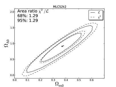
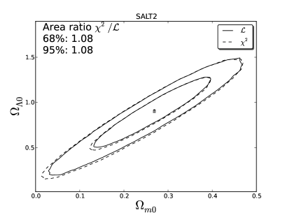
Figure 1: 68% and 95% confidence level contours, in the plane $\Omega_{m0}\times\Omega_{\Lambda 0}$, for the $\Lambda$CDM model. We marginalized over all other parameters with flat prior. The solid (dashed) lines are the results for the likelihood ($\chi^{2}$) approach. The black circle (gray square) is the best fit value for the likelihood ($\chi^{2}$). Left panel: Results for the MLCS2k2 version of the SDSS compilation. Right panel: Results for the SALT2 version of the SDSS compilation.

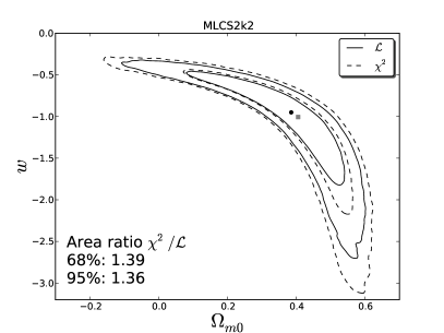
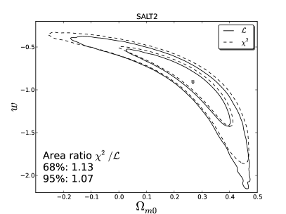
Figure 2: 68% and 95% confidence level contours, in the plane $\Omega_{m0}\times w$, for the F$w$CDM model. We marginalized over all other parameters with flat prior. The solid (dashed) lines are the results for the likelihood ($\chi^{2}$) approach. The black circle (gray square) is the best fit value for the likelihood ($\chi^{2}$). Left panel: Results for the MLCS2k2 version of the SDSS compilation. Right panel: Results for the SALT2 version of the SDSS compilation.

In Fig. 3 we show the confidence contours for the SALT2 parameters $\boldsymbol{\delta}$ for both $\Lambda$CDM and F$w$CDM models. We can see that there is no significant difference in the constraints for $\alpha$. For $\beta$ we find a bias that is, however, small compared to the 68% confidence interval for this parameter.

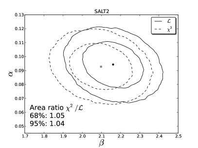
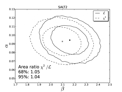
Figure 3: 68% and 95% confidence level contours in the plane $\beta\times\alpha$. We marginalized over all other parameters with flat prior. The solid (dashed) lines are the results for the likelihood ($\chi^{2}$) approach. The black circle (gray square) is the best fit value for the likelihood ($\chi^{2}$). Left panel: Results for the $\Lambda$CDM model with the SDSS compilation. Right panel: Results for the F$w$CDM model with the SDSS compilation.

In Fig. 4 we show the probability distributions for $\sigma_{\text{int}}$, given by the likelihood approach, for MLCS2k2 and SALT2 data. The traditional $\chi^{2}$ approach gives only one value for this parameter without uncertainty and we represent it by the dashed vertical line in the figure. We can see that the discrepancy between the value obtained from the $\chi^{2}$ approach and the best fit value obtained from the likelihood approach is greater for the MLCS2k2 data. The results are incompatible at more than 99% confidence interval, which does not happen for the SALT2 data. This can possibly be due to the fact that $\sigma_{\text{int}}$ is obtained using only a nearby sample in the $\chi^{2}$ approach for MLCS2k2 while such distinction is not performed in the likelihood approach. This issue deserves further investigation and will be the subject of future work.

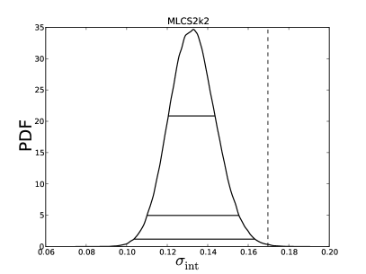
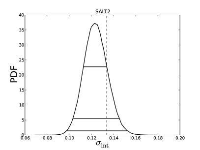
Figure 4: Distributions for $\sigma_{\text{int}}$ for the $\Lambda$CDM model from the likelihood approach. We marginalized over all other parameters with flat prior. The horizontal lines depict the 68%, 95% and 99% confidence intervals. The dashed line is the result for the $\chi^{2}$ approach. Left panel: Results for the MLCS2k2 version of the SDSS compilation. Right panel: Results for the SALT2 version of the SDSS compilation.

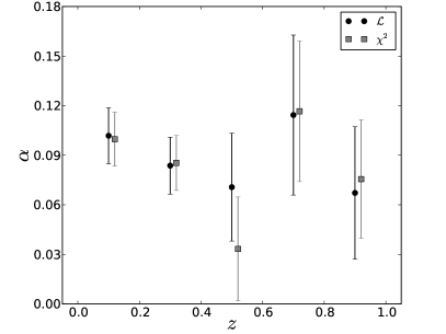
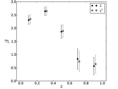
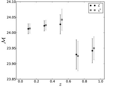
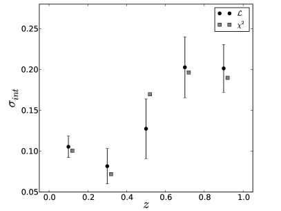
Figure 5: Evolution of SALT2 parameters $\alpha$, $\beta$, ${\cal M}$, and $\sigma_{\rm int}$ with redshift for the SDSS compilation for model $\Lambda$CDM. The cosmological parameters were kept fixed in their global best fit values. The black circles and the gray squares are the results for the likelihood and the $\chi^{2}$ approaches, respectively. The error bars represent the 68% confidence intervals, marginalizing over all other parameters with flat priors.

We also allow for a possible variation of the parameters $\alpha$, $\beta$, $\mathcal{M}$ and $\sigma_{\mathrm{int}}$ with redshift, in the context of the SALT2 data. In order to perform such analysis the dataset was divided in redshift bins and the cosmological parameters were fixed in the best-fit values obtained from the global fit, then releasing $\alpha$, $\beta$, $\mathcal{M}$ and $\sigma_{\text{int}}$ to be determined in each bin. The results are shown in Fig. 5. We found evidence of evolution for the parameter $\beta$, in agreement with (Kessler, 2009); furthermore we also found evidence of evolution for $\sigma_{\text{int}}$, which might support the use of a variable $\sigma_{\text{int}}$ instead of a constant one.

In addition to the SDSS compilation, we also used the Union2 compilation (Amanullah, 2010) and the SNLS third year data (Guy, 2011). However these references do not provide the covariances between the SALT2 parameters ($m_{B}^{*}$,$x_{1}$,$c$). In order to make a fair comparison with the SDSS data, we ran again the analyses for all three samples, this time neglecting the cross terms in Eq. (14). Without taking into account the covariances, the differences in the areas for the SDSS compilation are essentially the same. The main difference relies on the fact that, for the F$w$CDM model, the constraints are tighter for the $\chi^{2}$ approach than for the likelihood one. For the Union 2 compilation, the difference in the areas ranged from 13% to 14%, while the SNLS data showed the greater discrepancies, reaching up to $\sim$53%.

6 Conclusion

In this work we considered the SDSS first year compilation and compared two different approaches (traditional $\chi^{2}$ and likelihood) to determine constraints from SN Ia processed by two of the most used light curve fitters in the literature, the MLCS2k2 and the SALT2. The MLCS2k2 gives a cosmology-independent estimation of the distance modulus for each SN Ia, with its corresponding variance, which can be directly compared with the model prediction for this quantity. The SALT2 is not a distance estimator, consequently, we can only have an estimate of the distance modulus depending on parameters to be obtained simultaneously with the cosmological ones. Furthermore, in the SNe Ia analysis, it is common to introduce a residual, unknown, contribution $\sigma_{\text{int}}$ to the variance which, in the traditional approach, is determined by imposing that the reduced $\chi^{2}$ be unity, when considering the full sample, in the SALT2 case, or only nearby SNe Ia, in the MLCS2k2 case.

By comparing the results obtained from the traditional $\chi^{2}$ approach with the likelihood ones, we showed that, for current data and chosen cosmological models, there is a small difference in the best fit values and confidence contours ($\sim$ 30% difference in area) (cf. Figs. 1 and 2) in case the MLCS2k2 fitter is adopted. For SALT2 the difference is less significant ($\lesssim 13\%$ difference in areas). In both cases the likelihood approach gives more restrictive constraints. We can understand these results by observing, from Fig. 4, that the estimated value of $\sigma_{\text{int}}$ in the traditional approach, is higher than the peak of the $\sigma_{\text{int}}$ distribution obtained with the likelihood method. In fact, for MLCS2k2 the $\sigma_{\text{int}}$ value obtained with the traditional $\chi^{2}$ approach is outside the 99% confidence level of the distribution obtained with the likelihood method. For SALT2 it is of the order of 68% confidence level and this might explain why for SALT2 the differences between these two approaches are less significant. We should also remark that we noticed that the covariance between the SALT2 parameters ($m^{*}_{B},x_{1},c$) has an important role in the above result since we obtained, for the 68% confidence level contour, an area ratio of 1.13, when considering the covariance, and of 0.95, when neglecting the covariance.

We also studied the possible evolution of the SALT2 parameters $\alpha$, $\beta$ and $\mathcal{M}$ with the redshift, splitting the samples in redshift bins and performing the fit separately for each one. In this situation, we found evidence of evolution in the parameter $\beta$ and also in $\sigma_{\text{int}}$.

While this paper was in preparation two articles addressing the issue of using $\chi^{2}$ with unknown variances appeared in the arXiv. The first one (Kim, 2011) focused on the question of the determination of $\sigma_{\text{int}}$, using simulated data for the distance modulus. The second one (March, 2011) studied the SALT2 case and proposed a sophisticated Bayesian analysis. We did not find in our work with the SDSS first year compilation any kind of catastrophic biases of parameters when adopting the likelihood approach, a possibility suggested in (March, 2011).

In summary, we used current data to compare the traditional $\chi^{2}$ and the likelihood approaches to determine best fit and confidence regions from SN Ia. We argued that when the variance is not completely known, minimizing the traditional $\chi^{2}$ is not formally equivalent to maximizing the likelihood function, since the normalization of the likelihood, assumed Gaussian, is also a function of parameters to be determined. We conclude suggesting the adoption of the likelihood framework instead of the traditional $\chi^{2}$ one, since it is more straightforward, numerically more efficient and self-consistent.

7 Acknowledgments

We would like to thank Masao Sako for helpful discussions and suggestions. B. L. L. and I. W. also thank CNPq, Brazil, and S. E. J. also thanks ICTP, Italy, for support.

References

- Amanullah (2010) R. Amanullah et alii, Astrophys. J. 716, 712 (2010) [arXiv:1004.1711].
- Antcheva (2009) I. Antcheva et alii, Comput. Phys. Commun., 180, 2499 (2009).
- Astier (2006) P. Astier et alii, Astron. Astrophys. 447, 31 (2006) [astro-ph/0510447] [SNLS1].
- Burns (2011) C. R. Burns et alii, Astron. J. 141, 19 (2011) [arXiv:1010.4040].
- Conley (2008) A. Conley et alii, Astrophys. J. 681, 482 (2008) [arXiv:0803.3441].
- Conley (2011) A. Conley et alii, Astrophys. J. Suppl. 192, 1 (2011) [arXiv:1104.1443].
- Contardo (2000) G. Contardo, B. Leibundgut, and W. D. Vacca, Astron. Astrophys. 359, 876 (2000) [astro-ph/0005507].
- Davis (2010) T. M. Davis et alii, [arXiv:1012.2912].
- (9) DES: http://www.darkenergysurvey.org/.
- Dilday (2010) B. Dilday et alii, Astrophys. J. 713, 1026 (2010) [arXiv:1001.4995].
- Eisenstein (2005) D. J. Eisenstein et alii, Astrophys. J. 633, 560 (2005) [astro-ph/0501171].
- Faccioli (2011) L. Faccioli et alii, Astropart. Phys. 34, 847 (2011) [arXiv:1004.3511].
- Goobar (2011) A. Goobar and B. Leibundgut, accepted in Annu. Rev. Nucl. Part. Sci. [arXiv:1102.1431].
- Gupta (2011) R. R. Gupta, [arXiv:1107.6003].
- Guy (2005) J. Guy et alii, Astron. Astrophys. 443, 781 (2005) [astro-ph/0506583].
- Guy (2007) J. Guy et alii, Astron. Astrophys. 466, 11 (2007) [astro-ph/0701828].
- Guy (2011) J. Guy et alii, Astron. Astrophys. 523, A7 (2010) [arXiv:1010.4743] [SNLS3a].
- Hamuy (1996) M. Hamuy et alii, Astron. J. 112, 2391 (1996) [astro-ph/9609059].
- Hayden (2010) B. T. Hayden et alii, Astrophys. J. 722, 1691 (2010) [arXiv:1008.4797].
- Hicken (2009) M. Hicken et alii, Astrophys. J. 700, 1097 (2009) [arXiv:0901.4804].
- Hillebrandt (2000) W. Hillebrandt and J. C. Niemeyer, Annu. Rev. Astron. Astrophys. 38, 191 (2000) [astro-ph/0203369].
- Howell (2011) D. A. Howell, Nature Commun. 2, 350 (2011) [arXiv:1011.0441].
- Hsiao (2007) E. Y. Hsiao et alii, Astrophys. J. 663, 1187 (2007) [astro-ph/0703529].
- Hui (2006) L. Hui and P. B. Greene, Phys. Rev D 73, 123526 (2006) [astro-ph/512159].
- James (1975) F. James and M. Roos, Comput. Phys. Commun., 10, 343 (1975).
- Jha (2007) S. Jha, A. G. Riess and R. P. Kirshner, Astrophys. J. 659, 122 (2007) [astro-ph/0612666].
- Kessler (2009) R. Kessler et alii, Astrophys. J. Suppl. 185, 32 (2009) [arXiv:0908.4274].
- Kim (2011) A. G. Kim, accepted by Publications of the Astronomical Society of the Pacific, [arXiv:1101.3513].
- Kirshner (2010) R. P. Kirshner, in Dark energy. Observational and theoretical approaches, edited by P. Ruiz-Lapuente [arXiv:0910.0257].
- Komatsu (2011) E. Komatsu et alii, Astrophys. J. Suppl. 192, 18 (2011) [arXiv:1001.4538].
- Kowalski (2008) M. Kowalski et alii, Astrophys. J. 686, 749 (2008) [arXiv:0804.4142].
- Kronborg (2010) T. Kronborg et alii, [arXiv:1002.1249].
- Lampeitl (2010) H. Lampeitl et alii, Astrophys. J. 722, 566 (2010) [arXiv:1005.4687].
- (34) LSST: http://www.lsst.org/.
- Mantz (2010) A. Mantz et alii, Mon. Not. Roy. Astron. Soc. 406, 1759 (2010) [arXiv:0909.3098].
- Maoz (2010) D. Maoz, [arXiv:1011.1014].
- March (2011) M. C. March et alii, accepted by Mon. Not. Roy. Astron. Soc. [arXiv:1102.3237].
- Nobili (2009) S. Nobili et alii, Astrophys. J. 700, 1415 (2009) [arXiv:0906.4318].
- Nugent (2002) P. Nugent, A. Kim and S. Perlmutter, Pub. Astron. Soc. Pacific 114, 803 (2002) [astro-ph/0205351].
- (40) Pan-STARRS: http://pan-starrs.ifa.hawaii.edu/.
- Percival (2010) W. J. Percival et alii, Mon. Not. Roy. Astron. Soc. 401, 2148 (2010) [arXiv:0907.1660].
- Perlmutter (1999) S. Perlmutter et alii, Astrophys. J. 517, 565 (1999) [astro-ph/9812133].
- Phillips (1993) M. M. Phillips, Astrophys. J. 413, L105 (1993).
- Riess (1998) A. G. Riess et alii, Astron. J. 116, 1009 (1998) [astro-ph/9805201].
- Sullivan (2010) M. Sullivan et alii, Mon. Not. R. Astron. Soc. 406, 782 (2010) [arXiv:1003.5119].
- Vaughan (1995) T. E. Vaughan et alii, Astrophys. J. 439, 558 (1995).
- Vikhlinin (2009) A. Vikhlinin et alii, Astrophys. J. 692, 1060 (2009) [arXiv:0812.2720].
- Vishwakarma (2010) R. G. Vishwakarma and J. V. Narlikar, Res. Astron. Astrophys. 10, 1195 (2010) [arXiv:1010.5272].
- Wang (2003) L. Wang et alii,Astrophys. J. 590, 944 (2003) [astro-ph/0302341].
- Wang (2005) X. Wang et alii, Astrophys. J. 620, L87 (2005) [astro-ph/0501565].
- Wang (2005) Y. Wang, J. Cosmol. Astropart. Phys. 03 (2005), 005 [astro-ph/0406635].
- Wood-Vasey (2007) W. M. Wood-Vasey et alii, Astrophys. J. 666, 694 (2007) [astro-ph/0701041].
- Yasuda (2010) N. Yasuda and M. Fukugita, Astron. J. 139, 39 (2010) [arXiv:0905.4125].