QCD for Collider Physics

Abstract

These lectures are directed at a level suitable for graduate students in experimental and theoretical High Energy Physics. They are intended to give an introduction to the theory and phenomenology of quantum chromodynamics (QCD) as it is used in collider physics applications. The aim is to bring the reader to a level where informed decisions can be made concerning different approaches and their uncertainties. The material is divided into four main areas: 1) fundamentals, 2) perturbative QCD, 3) soft QCD, and 4) Monte Carlo event generators.

1 Introduction

When probed at very short wavelengths, QCD is essentially a theory of free ‘partons’ — quarks and gluons — which only scatter off one another through relatively small quantum corrections, that can be systematically calculated. At longer wavelengths, of order the size of the proton $\sim 1\mathrm{fm}=10^{-15}\mathrm{m}$, however, we see strongly bound towers of hadron resonances emerge, with string-like potentials building up if we try to separate their partonic constituents. Due to our inability to solve strongly coupled field theories, QCD is therefore still only partially solved. Nonetheless, all its features, across all distance scales, are believed to be encoded in a single one-line formula of alluring simplicity; the Lagrangian of QCD.

The consequence for collider physics is that some parts of QCD can be calculated in terms of the fundamental parameters of the Lagrangian, whereas others must be expressed through models or functions whose effective parameters are not a priori calculable but which can be constrained by fits to data. However, even in the absence of a perturbative expansion, there are still several strong theorems which hold, and which can be used to give relations between seemingly different processes. (This is, e.g., the reason it makes sense to constrain parton distribution functions in $ep$ collisions and then re-use the same ones for $pp$ collisions.) Thus, in the chapters dealing with phenomenological models we shall emphasize that the loss of a factorized perturbative expansion is not equivalent to a total loss of predictivity.

An alternative approach would be to give up on calculating QCD altogether and use leptons instead. Formally, this amounts to summing inclusively over strong-interaction phenomena, when such are present. While such a strategy might succeed in replacing what we do know about QCD by “unity”, however, even the most adamant “chromophobe” must acknowledge a few basic facts of collider physics for the next decade(s): 1) At the Tevatron and LHC, the initial states are unavoidably hadrons, and hence, at the very least, well-understood and precise parton distribution functions (PDFs) will be required; 2) high precision will mandate calculations to higher orders in perturbation theory, which in turn will involve more QCD; 3) the requirement of lepton isolation makes the very definition of a lepton depend implicitly on QCD, and 4) the rate of jets that are misreconstructed as leptons in the experiment depends explicitly on it. Finally, 5) though many new-physics signals do give observable signals in the lepton sector, this is far from guaranteed. It would therefore be unwise not to attempt to solve QCD to the best of our ability, the better to prepare ourselves for both the largest possible discovery reach and the highest attainable subsequent precision.

In the following, we shall focus squarely on QCD for mainstream collider physics. This includes factorization, hard processes, infrared safety, parton showers and matching, event generators, hadronization, and the so-called underlying event. While not covering everything, hopefully these topics can also serve at least as stepping stones to more specialized issues that have been left out, such as heavy flavours or forward physics, or to topics more tangential to other fields, such as lattice QCD or heavy-ion physics.

1.1 A First Hint of Colour

Looking for new physics, as we do now at the LHC, it is instructive to consider the story of the discovery of colour. The first hint was arguably the $\Delta^{++}$ baryon, found in 1951 [1]. The title and part of the abstract from this historical paper are reproduced in figure 1.

“[…] It is concluded that the apparently anomalous features of the scattering can be interpreted to be an indication of a resonant meson-nucleon interaction corresponding to a nucleon isobar with spin $\frac{3}{2}$, isotopic spin $\frac{3}{2}$, and with an excitation energy of $277\,$MeV.”

Figure 1: The title and part of the abstract of the 1951 paper [1] (published in 1952) in which the discovery of the $\Delta^{++}$ baryon was announced.

In the context of the quark model — which first had to be developed, successively joining together the notions of spin, isospin, strangeness, and the eightfold way — the flavour and spin content of the $\Delta^{++}$ baryon is:

$$\left|\Delta^{++}\right>=\left|\,u_{\uparrow}\ u_{\uparrow}\ u_{\uparrow}\right>~{},$$ (1)

clearly a highly symmetric configuration. However, since the $\Delta^{++}$ is a fermion, it must have an overall antisymmetric wave function. In 1965, fourteen years after its discovery, this was finally understood by the introduction of colour as a new quantum number associated with the group SU(3) [2, 3]. The $\Delta^{++}$ wave function can now be made antisymmetric by arranging its three quarks antisymmetrically in this new degree of freedom,

$$\left|\Delta^{++}\right>=\epsilon^{ijk}\left|\,u_{i\uparrow}\ u_{j\uparrow}\ u_{k\uparrow}\right>~{},$$ (2)

hence solving the mystery.

More direct experimental tests of the number of colours were provided first by measurements of the decay width of $\pi^{0}\to\gamma\gamma$ decays, which is proportional to $N_{C}^{2}$, and later by the famous “R” ratio in $e^{+}e^{-}$ collisions. Below, in Section 1.2 we shall see how to calculate such colour factors.

1.2 The Lagrangian of QCD

Quantum Chromodynamics is based on the gauge group $\mathrm{SU(3)}$, the Special Unitary group in 3 (complex) dimensions. In the context of QCD, we represent this group as a set of unitary $3\times 3$ matrices with determinant one. This is called the adjoint representation and can be used to represent gluons in colour space. Since there are 9 linearly independent unitary complex matrices, one of which has determinant $-1$, there are a total of 8 independent directions in the adjoint colour space, i.e., the gluons are octets. In QCD, these matrices can operate both on each other (gluon self-interactions) and on a set of complex $3$-vectors (the fundamental representation), the latter of which represent quarks in colour space. The fundamental representation has one linearly independent basis vector per degree of $\mathrm{SU(3)}$, and hence the quarks are triplets.

The Lagrangian of QCD is

$${\cal L}=\bar{\psi}_{q}^{i}(i\gamma^{\mu})(D_{\mu})_{ij}\psi_{q}^{j}-m_{q}\bar{\psi}_{q}^{i}\psi_{qi}-\frac{1}{4}F^{a}_{\mu\nu}F^{a\mu\nu}~{},$$ (3)

where $\psi_{q}^{i}$ denotes a quark field with colour index $i$, $\psi_{q}=({{\color[rgb]{1,0,0}\psi_{qR}}},{\color[rgb]{0,1,0}\psi_{qG}},{\color[rgb]{0,0,1}\psi_{qB}})^{T}$, $\gamma^{\mu}$ is a Dirac matrix that expresses the vector nature of the strong interaction, with $\mu$ being a Lorentz vector index, $m_{q}$ allows for the possibility of non-zero quark masses (induced by the standard Higgs mechanism or similar), $F^{a}_{\mu\nu}$ is the gluon field strength tensor for a gluon with colour index $a$ (in the adjoint representation, i.e., $a\in[1,\ldots,8]$), and $D_{\mu}$ is the covariant derivative in QCD,

$$(D_{\mu})_{ij}=\delta_{ij}\partial_{\mu}-ig_{s}t_{ij}^{a}A_{\mu}^{a}~{},$$ (4)

with $g_{s}$ the strong coupling (related to $\alpha_{s}$ by $g_{s}^{2}=4\pi\alpha_{s}$; we return to the strong coupling in more detail below), $A^{a}_{\mu}$ the gluon field with (adjoint-representation) colour index $a$, and $t_{ij}^{a}$ proportional to the hermitean and traceless Gell-Mann matrices of $\mathrm{SU(3)}$,

$$\mbox{\includegraphics*[scale={1.0}]{gell-mann}}~{}.$$ (5)

These generators are just the $\mathrm{SU(3)}$ analogs of the Pauli matrices in $\mathrm{SU(2)}$. By convention, the constant of proportionality is normally taken to be

$$t^{a}_{ij}=\frac{1}{2}\lambda^{a}_{ij}~{}.$$ (6)

This choice in turn determines the normalization of the coupling $g_{s}$, via equation (4), and fixes the values of the $\mathrm{SU(3)}$ Casimirs and structure constants, to which we return below.

An example of the colour flow for a quark-gluon interaction in colour space is given in figure 2.

$A^{1}_{\mu}$

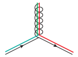
$\psi_{q{\color[rgb]{1,0,0}R}}$ $\psi_{q{\color[rgb]{0,1,0}G}}$

$\begin{array}[]{ccccc}\propto&-\frac{i}{2}g_{s}&\bar{\psi}_{q\color[rgb]{1,0,0}R}&\lambda^{1}&\psi_{q\color[rgb]{0,1,0}G}\\[5.69054pt] =&-\frac{i}{2}g_{s}&\left(\begin{array}[]{ccc}{\color[rgb]{1,0,0}1}&\color[rgb]{0,1,0}0&\color[rgb]{0,0,1}0\end{array}\right)&\left(\begin{array}[]{ccc}0&1&0\\ 1&0&0\\ 0&0&0\end{array}\right)&\left(\begin{array}[]{c}{\color[rgb]{1,0,0}0}\\ \color[rgb]{0,1,0}1\\ \color[rgb]{0,0,1}0\end{array}\right)\end{array}$

Figure 2: Illustration of a $qqg$ vertex in QCD, before summing/averaging over colours: a gluon in a state represented by $\lambda^{1}$ interacts with quarks in the states $\psi_{qR}$ and $\psi_{qG}$.

Typically, however, we do not measure colour in the final state — instead we average over all possible incoming colours and sum over all possible outgoing ones, wherefore QCD scattering amplitudes (squared) in practice always contain sums over quark fields contracted with Gell-Mann matrices. These contractions in turn produce traces which yield the colour factors that are associated to each QCD process, and which basically count the number of “paths through colour space” that the process at hand can take, modulo that the convention choice represented by equation (6) introduces a “spurious” factor of 2 for each power of the coupling $\alpha_{s}$, as we shall see.

A very simple example of a colour factor is given by the decay process $Z\to q\bar{q}$. This vertex contains a simple $\delta_{ij}$ in colour space; the outgoing quark and antiquark must have identical (anti-)colours. Squaring the corresponding matrix element and summing over final-state colours yields a colour factor of

$$Z\to q\bar{q}~{}~{}~{}:~{}~{}~{}\sum_{\mathrm{colours}}|M|^{2}\propto\delta_{ij}\delta^{*}_{ji}=\mathrm{Tr}\{\delta\}=N_{C}=3~{},$$ (7)

since $i$ and $j$ are quark (i.e., 3-dimensional fundamental-representation) indices.

A next-to-simplest example is given by the Drell-Yan process, $q\bar{q}\to\gamma^{*}/Z$, i.e., just a crossing of the previous one. By crossing symmetry, the squared matrix element, including the colour factor, is exactly the same as before, but since the quarks are here incoming, we must average rather than sum over their colours, leading to

$$q\bar{q}\to Z~{}~{}~{}:~{}~{}~{}\frac{1}{9}\sum_{\mathrm{colours}}|M|^{2}\propto\frac{1}{9}\delta_{ij}\delta^{*}_{ji}=\frac{1}{9}\mathrm{Tr}\{\delta\}=\frac{1}{3}~{},$$ (8)

where the colour factor now expresses a suppression which can be interpreted as due to the fact that only quarks of matching colours are able to collide and produce a $Z$ boson, effectively reducing the incoming quark-antiquark flux by a factor 1/$N_{C}$.

To illustrate what happens when we insert (and sum over) quark-gluon vertices, such as the one depicted in figure 2, we take the process $Z\to 3\,$jets. The colour factor for this process can be computed as follows, with the accompanying illustration showing a corresponding diagram (squared) with explicit colour-space indices on each vertex:

$$Z\to qg\bar{q} \begin{array}[]{rcl}\displaystyle\sum_{\mathrm{colours}}|M|^{2}&\propto&\displaystyle\delta_{ij}t_{jk}^{a}\left(t_{\ell k}^{a}\delta^{*}_{i\ell}\right)^{*}\\ &=&\displaystyle\mathrm{Tr}\{t^{a}t^{a}\}\\[11.38109pt] &=&\displaystyle\frac{1}{2}\mathrm{Tr}\{\delta\}=4~{},\end{array}$$   : (9)

where the last $\mathrm{Tr}\{\delta\}=8$, since the trace runs over indices in the 8-dimensional adjoint representation.

The tedious task of taking traces over $\mathrm{SU(3)}$ matrices can be greatly alleviated by use of the relations given in Table 1.

Trace Relation	Indices	Occurs in Diagram Squared
$\mathrm{Tr}\{t^{a}t^{b}\}=T_{R}\,\delta^{ab}$	$a,b\in[1,\ldots,8]$
$\sum_{a}t^{a}_{ij}t^{a}_{jk}=C_{F}\,\delta_{ik}$	$a\in[1,\ldots,8]$ $i,j,k\in[1,\ldots,3]$
$\sum_{c,d}f^{acd}f^{bcd}=C_{A}\,\delta^{ab}$	$a,b,c,d\in[1,\ldots,8]$
$t^{a}_{ij}t^{a}_{k\ell}=T_{R}\left(\delta_{jk}\delta_{i\ell}-\frac{1}{N_{C}}\delta_{ij}\delta_{k\ell}\right)$	$i,j,k,\ell\in[1,\ldots,3]$	(Fierz)

Table 1: Trace relations for $t$ matrices. These relations are convention-independent as they stand. Relations for a specific normalization convention for the $t$ matrices are obtained by inserting the specific values of $T_{R}$, $C_{F}$, and $C_{A}$ pertaining to that convention choice, as discussed in the text. More relations can be found in [4, Section 1.2] and in [5, Appendix A.3].

In the standard normalization convention for the $\mathrm{SU(3)}$ generators, equation (6), the Casimirs of $\mathrm{SU(3)}$ appearing in Table 1 are

$$T_{R}=\frac{1}{2}\hskip 56.9055ptC_{F}=\frac{4}{3}\hskip 56.9055ptC_{A}=N_{C}=3~{}.$$ (10)

In addition, the gluon self-coupling on the third line in Table 1 involves factors of $f^{abc}$. These are called the structure constants of QCD and they enter due to the non-Abelian term in the gluon field strength tensor appearing in equation (3),

$$F^{a}_{\mu\nu}=\partial_{\mu}A_{\nu}^{a}-\partial_{\nu}A^{a}_{\mu}+g_{s}f^{abc}A_{\mu}^{b}A_{\nu}^{c}~{}.$$ (11)

The structure constants of $\mathrm{SU(3)}$ are listed in the table to the right. Expanding the $F_{\mu\nu}F^{\mu\nu}$ term of the Lagrangian using equation (11), we see that there is a 3-gluon and a 4-gluon vertex that involve $f^{abc}$, the latter of which has two powers of $f$ and two powers of the coupling.

Finally, the last line of Table 1 is not really a trace relation but instead a useful so-called Fierz transformation. It is often used, for instance, in shower Monte Carlo applications, to assist in mapping between colour flows in $N_{C}=3$, in which cross sections and splitting probabilities are calculated, and those in $N_{C}\to\infty$, used to represent colour flow in the MC “event record”.

Structure Constants of $\mathrm{SU(3)}$ $$f_{123}=1$$ (12) $$f_{147}=f_{246}=f_{257}=f_{345}=\frac{1}{2}$$ (13) $$f_{156}=f_{367}=-\frac{1}{2}$$ (14) $$f_{458}=f_{678}=\frac{\sqrt{3}}{2}$$ (15) Antisymmetric in all indices All other $f_{ijk}=0$ (valid for the convention $t=\frac{\lambda}{2}$)
(for the alternative convention $t=\frac{\lambda}{\sqrt{2}}$, multiply all $f_{ijk}$ by $\sqrt{2}$)

$A_{\nu}^{4}(k_{2})$

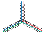
$A^{6}_{\rho}(k_{1})$ $A_{\mu}^{2}(k_{3})$

$\begin{array}[]{cccc}\propto&-g_{s}\ f^{246}\!\!&\!\![(k_{3}-k_{2})^{\rho}g^{\mu\nu}\\ &&+(k_{2}-k_{1})^{\mu}g^{\nu\rho}\\ &&+(k_{1}-k_{3})^{\nu}g^{\rho\mu}]\end{array}$

Figure 3: Illustration of a $ggg$ vertex in QCD, before summing/averaging over colours: interaction between gluons in the states $\lambda^{2}$, $\lambda^{4}$, and $\lambda^{6}$ is represented by the structure constant $f^{246}$.

A gluon self-interaction vertex is illustrated in figure 3, to be compared with the quark-gluon one in figure 2. We remind the reader that gauge boson self-interactions are a hallmark of non-Abelian theories and that their presence leads to some of the main differences between QED and QCD. One should also keep in mind that the colour factor for the vertex in figure 3, $C_{A}$, is roughly twice as large as that for a quark, $C_{F}$.

1.3 The Strong Coupling

To first approximation, QCD is scale invariant. That is, if one “zooms in” on a QCD jet, one will find a repeated self-similar pattern of jets within jets within jets, reminiscent of fractals such as the famous Mandelbrot set in mathematics, or the formation of frost crystals in physics. In the context of QCD, this property was originally called light-cone scaling, or Bjorken scaling after the famous physicist James D. Bjorken. It has since been rebranded by a new generation as conformal invariance, a mathematical property of several QCD-“like” theories which are now being studied. It is also closely related to the physics of so-called “unparticles”, though that is a relation that goes beyond the scope of these lectures.

Regardless of the labeling, if the strong coupling did not run (we shall return to the running of the coupling below), Bjorken scaling would be absolutely true. QCD would be a theory with a fixed coupling, the same at all scales. This simplified picture already captures some of the most important properties of QCD, as we shall discuss presently.

In the limit of exact Bjorken scaling — QCD at fixed coupling — properties of high-energy interactions are determined only by dimensionless kinematic quantities, such as scattering angles (pseudorapidities) and ratios of energy scales. For applications of QCD to high-energy collider physics, an important consequence of Bjorken scaling is thus that the rate of bremsstrahlung jets with a given transverse momentum scales in direct proportion to the hardness of the fundamental partonic scattering process they are produced in association with. For instance, in the limit of exact scaling, a measurement of the rate of 5-GeV jets produced in association with an ordinary $Z$ boson could be used as a direct prediction of the rate of 50-GeV jets that would be produced in association with a 900-GeV $Z^{\prime}$ boson, and so forth. Our intuition about how many bremsstrahlung jets a given type of process is likely to have should therefore be governed first and foremost by the ratios of scales that appear in that particular process, as has been highlighted in a number of studies focusing on the mass and $p_{\perp}$ scales appearing, e.g., in Beyond-the-Standard-Model (BSM) physics processes [6, 7, 8, 9, 10]. Bjorken scaling is also fundamental to the understanding of jet substructure in QCD, see, e.g., [11].

In real QCD, the coupling runs logarithmically with the energy,

$$Q^{2}\frac{\partial\alpha_{s}}{\partial Q^{2}}=\frac{\partial\alpha_{s}}{\partial\ln Q^{2}}=\beta(\alpha_{s})~{},$$ (16)

where the function driving the energy dependence, the beta function, is defined as

$$\beta(\alpha_{s})=-\alpha_{s}^{2}(b_{0}+b_{1}\alpha_{s}+b_{2}\alpha_{s}^{2}+\ldots)~{},$$ (17)

with LO (1-loop) and NLO (2-loop) coefficients

$$b_{0} = \frac{11C_{A}-4T_{R}n_{f}}{12\pi}~{},$$ (18)

$$b_{1} = \frac{17C_{A}^{2}-10T_{R}C_{A}n_{f}-6T_{R}C_{F}n_{f}}{24\pi^{2}}~{}=~{}\frac{153-19n_{f}}{24\pi^{2}}~{}.$$ (19)

Numerically, the value of the strong coupling is usually specified by giving its value at the specific reference scale $Q^{2}=M^{2}_{Z}$, from which we can obtain its value at any other scale by solving equation (16),

$$\alpha_{s}(Q^{2})=\alpha_{s}(M_{Z}^{2})\frac{1}{1+b_{0}\alpha_{s}(M_{Z}^{2})\ln\frac{Q^{2}}{M_{Z}^{2}}+{\cal O}(\alpha_{s}^{2})}~{},$$ (20)

with relations including the ${\cal O}(\alpha_{s}^{2})$ terms available, e.g., in [4]. Relations between scales not involving $M_{Z}^{2}$ can obviously be obtained by just replacing $M_{Z}^{2}$ by some other scale $Q^{\prime 2}$ everywhere in equation (20). As an application, let us prove that the logarithmic running of the coupling implies that an intrinsically multi-scale problem can be converted to a single-scale one, up to corrections suppressed by two powers of $\alpha_{s}$, by taking the geometric mean of the scales involved. This follows from expanding an arbitrary product of individual $\alpha_{s}$ factors around an arbitrary scale $\mu$, using equation (20),

$$\alpha_{s}(\mu_{1})\alpha_{s}(\mu_{2})\cdots\alpha_{s}(\mu_{n}) = \prod_{i=1}^{n}\alpha_{s}(\mu)\left(1+b_{0}\,\alpha_{s}\ln\left(\frac{\mu^{2}}{\mu_{i}^{2}}\right)+{\cal O}(\alpha_{s}^{2})\right)$$ (21)

$$= \alpha_{s}^{n}(\mu)\left(1+b_{0}\,\alpha_{s}\ln\left(\frac{\mu^{2n}}{\mu_{1}^{2}\mu_{2}^{2}\cdots\mu_{n}^{2}}\right)+{\cal O}(\alpha_{s}^{2})\right)~{},$$

whereby the specific single-scale choice $\mu^{n}=\mu_{1}\mu_{2}\cdots\mu_{n}$ (the geometric mean) can be seen to push the difference between the two sides of the equation one order higher than would be the case for any other combination of scales.

The appearance of the number of flavours, $n_{f}$, in $b_{0}$ implies that the slope of the running depends on the number of contributing flavours. Since full QCD is best approximated by $n_{f}=3$ below the charm threshold, by $n_{f}=4$ from there to the $b$ threshold, and by $n_{f}=5$ above that, it is therefore important to be aware that the running changes slope across quark flavour thresholds. Likewise, it would change across the threshold for top or for any coloured new-physics particles that might exist, with a magnitude depending on the particles’ colour and spin quantum numbers.

The negative overall sign of equation (17), combined with the fact that $b_{0}>0$, leads to the famous result that the QCD coupling effectively decreases with energy, called asymptotic freedom, for the discovery of which the Nobel prize in physics was awarded to D. Gross, H. Politzer, and F. Wilczek in 2004. An extract of the prize announcement runs as follows:

What this year’s Laureates discovered was something that, at first sight, seemed completely contradictory. The interpretation of their mathematical result was that the closer the quarks are to each other, the weaker is the “colour charge”. When the quarks are really close to each other, the force is so weak that they behave almost as free particles. This phenomenon is called “asymptotic freedom”. The converse is true when the quarks move apart: the force becomes stronger when the distance increases.

Among the consequences of asymptotic freedom is that perturbation theory becomes better behaved at higher absolute energies, due to the effectively decreasing coupling. Perturbative calculations for our 900-GeV $Z^{\prime}$ boson from before should therefore be slightly faster converging than equivalent calculations for the 90-GeV one. Furthermore, since the running of $\alpha_{s}$ explicitly breaks Bjorken scaling, we also expect to see small changes in jet shapes and in jet production ratios as we vary the energy. For instance, since high-$p_{\perp}$ jets start out with a smaller effective coupling, their intrinsic shape (irrespective of boost effects) is somewhat narrower than for low-$p_{\perp}$ jets, an issue which can be important for jet calibration. Our current understanding of the running of the QCD coupling is summarized by the plot in figure 4, taken from a recent comprehensive review by S. Bethke [12].

As a final remark on asymptotic freedom, note that the decreasing value of the strong coupling with energy must eventually cause it to become comparable to the electromagnetic and weak ones, at some energy scale. Beyond that point, which may lie at energies of order $10^{15}-10^{17}\,$GeV (though it may be lower if as yet undiscovered particles generate large corrections to the running), we do not know what the further evolution of the combined theory will actually look like, or whether it will continue to exhibit asymptotic freedom.

Now consider what happens when we run the coupling in the other direction, towards smaller energies.

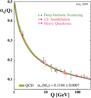
Figure 4: Illustration of the running of $\alpha_{s}$ in a theoretical calculation (yellow shaded band) and in physical processes at different characteristic scales, from [12].

Taken at face value, the numerical value of the coupling diverges rapidly at scales below 1 GeV, as illustrated by the curves disappearing off the left-hand edge of the plot in figure 4. To make this divergence explicit, one can rewrite equation (20) in the following form,

$$\alpha_{s}(Q^{2})=\frac{1}{b_{0}\ln\frac{Q^{2}}{\Lambda^{2}}}~{},$$ (22)

where

$$\Lambda\sim 200\,\mbox{GeV}$$ (23)

specifies the energy scale at which the perturbative coupling would nominally become infinite, called the Landau pole. (Note, however, that this only parametrizes the purely perturbative result, which is not reliable at strong coupling, so equation (22) should not be taken to imply that the physical behaviour of full QCD should exhibit a divergence for $Q\to\Lambda$.)

Finally, one should be aware that there is a multitude of different ways of defining both $\Lambda$ and $\alpha_{s}(M_{Z})$. At the very least, the numerical value one obtains depends both on the renormalization scheme used (with the dimensional-regularization-based “modified minimal subtraction” scheme, $\overline{\mbox{MS}}$, being the most common one) and on the perturbative order of the calculations used to extract them. As a rule of thumb, fits to experimental data typically yield smaller values for $\alpha_{s}(M_{Z})$ the higher the order of the calculation used to extract it (see, e.g., [12, 13]), with $\alpha_{s}(M_{Z})|_{\mathrm{LO}}\mathrel{\hbox to0.0pt{\lower 4.0pt\hbox{\hskip 1.0pt$\sim$}\hss}\raise 1.0pt\hbox{$>$}}\alpha_{s}(M_{Z})|_{\mathrm{NLO}}\mathrel{\hbox to0.0pt{\lower 4.0pt\hbox{\hskip 1.0pt$\sim$}\hss}\raise 1.0pt\hbox{$>$}}\alpha_{s}(M_{Z})|_{\mathrm{NNLO}}$. Further, since the number of flavours changes the slope of the running, the location of the Landau pole for fixed $\alpha_{s}(M_{Z})$ depends explicitly on the number of flavours used in the running. Thus each value of $n_{f}$ is associated with its own value of $\Lambda$, with the following matching relations across thresholds guaranteeing continuity of the coupling at one loop,

$$n_{f}=4\leftrightarrow 5~{}~{}~{}:~{}~{}~{}~{}~{}~{}\Lambda_{5}=\Lambda_{4}\left(\frac{\Lambda_{4}}{m_{b}}\right)^{\frac{2}{23}} \Lambda_{4}=\Lambda_{5}\left(\frac{m_{b}}{\Lambda_{5}}\right)^{\frac{2}{25}}~{},$$ (24)

$$n_{f}=3\leftrightarrow 4~{}~{}~{}:~{}~{}~{}~{}~{}~{}\Lambda_{4}=\Lambda_{3}\left(\frac{\Lambda_{3}}{m_{c}}\right)^{\frac{2}{25}} \Lambda_{3}=\Lambda_{4}\left(\frac{m_{c}}{\Lambda_{4}}\right)^{\frac{2}{27}}~{}.$$ (25)

It is sometimes stated that QCD only has a single free parameter, the strong coupling. Appealing as this may be, it is a bit of an overstatement. Even in the perturbative region, the beta function depends explicitly on the number of quark flavours, as we have seen, and thereby also on the quark masses. Furthermore, in the non-perturbative region around or below $\Lambda_{\mathrm{QCD}}$, the value of the perturbative coupling, as obtained, e.g., from equation (22), gives little or no insight into the behaviour of the full theory. Instead, universal functions (such as parton densities, form factors, fragmentation functions, etc), effective theories (such as the Operator Product Expansion, Chiral Perturbation Theory, or Heavy Quark Effective Theory), or phenomenological models (such as Regge Theory or the String and Cluster Hadronization Models) must be used, which in turn depend on additional non-perturbative parameters whose relation to, e.g., $\alpha_{s}(M_{Z})$, is not a priori known. For some of these questions, such as hadron masses, lattice QCD can furnish important additional insight, but for multi-scale and/or time-evolution problems, the applicability of lattice methods is still severely restricted.

2 Perturbative QCD

Our main tool for solving QCD for high-energy collider physics is perturbative quantum field theory, the starting point for which is Matrix Elements (MEs) which can be calculated systematically at fixed orders in the strong coupling $\alpha_{s}$. At least at lowest order (LO), the procedure is standard textbook material [5] and it has also by now been highly automated, by the advent of tools like CalcHep [14], CompHep [15], MadGraph [16], and others [17, 18, 19, 20, 21]. Here, we require only that the reader has a basic familiarity with the methods involved from graduate-level particle physics courses based, e.g., on [5, 22]. Our main concern are the uses to which these calculations are put, their limitations, and ways to improve on the results obtained with them.

For illustration, take one of the most commonly occurring processes in hadron collisions — Rutherford scattering of two quarks via a $t$-channel gluon exchange — which has the differential cross section

$$qq^{\prime}\to qq^{\prime}~{}~{}~{}:~{}~{}~{}\frac{\mathrm{d}\sigma\hskip 1.99997pt}{\mathrm{d}\hat{t}\hskip 1.99997pt}=\frac{\pi}{\hat{s}^{2}}\,\frac{4}{9}\,\alpha_{s}^{2}\,\frac{\hat{s}^{2}+\hat{u}^{2}}{\hat{t}^{2}}~{},$$ (26)

with the $2\to 2$ Mandelstam variables (“hatted” to emphasize that they refer to a partonic $2\to 2$ scattering rather than the full $pp\to\mbox{jets}$ process)

$$\hat{s} = (p_{1}+p_{2})^{2}~{},$$ (27)

$$\hat{t} = (p_{3}-p_{1})^{2}=-\hat{s}\frac{(1-\cos\hat{\theta})}{2}~{},$$ (28)

$$\hat{u} = (p_{4}-p_{1})^{2}=-\hat{s}\frac{(1+\cos\hat{\theta})}{2}~{}.$$ (29)

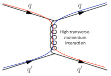
$p_{1}$ $p_{3}$ $p_{2}$ $p_{4}$

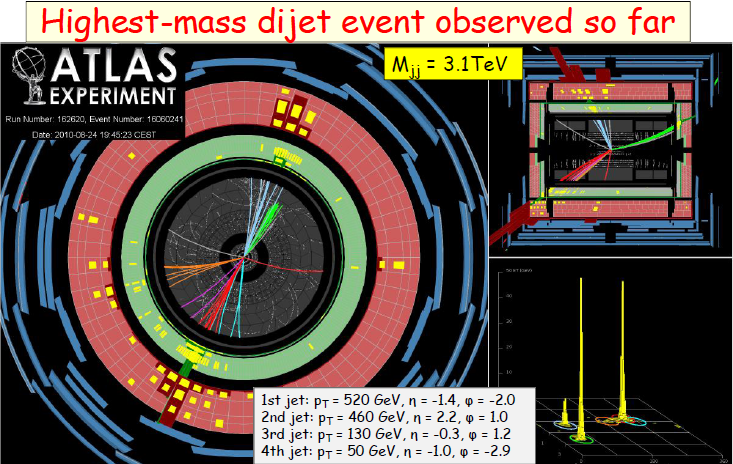
Figure 5: Left: Rutherford scattering of quarks in QCD, exemplifying the type of process that dominates the short-distance interaction cross section at hadron colliders. Right: an example of what such a reaction may look like in a detector, in this case the ATLAS experiment.

This process is illustrated in the left-hand pane of figure 5, including a rough (formally leading-$N_{C}$) representation of the “colour transfer” mediated by the gluon (as was discussed in Section 1.2).

Reality, however, is more complicated; the picture on the right-hand pane of figure 5 shows a real dijet event, as recorded by the ATLAS experiment. The complications to be addressed when going from left to right in figure 5 are: firstly, additional jets, a.k.a. real-emission corrections, which significantly change the topology of the final state, potentially shifting jets in or out of an experimentally defined acceptance region. Secondly, loop factors, a.k.a. virtual corrections, change the number of available quantum paths through phase space, and hence modify the normalization of the cross section (total and differential). And finally, additional corrections to the simple factorized perturbative picture are generated by components such as hadronization and the underlying event. These corrections must be taken into account to complete our understanding of QCD and connect the short-distance physics with macroscopic experiments. Apart from the perturbative expansion itself, the most powerful tool we have to organize this vast calculation, is factorization.

2.1 Factorization

When applicable, factorization allows us to subdivide the calculation of an observable into a perturbatively calculable short-distance part and an approximately universal long-distance part, the latter of which may be modeled and constrained by fits to data. Factorization can also be applied multiple times, to break up a complicated calculation into simpler pieces that can be treated as approximately independent, such as when dealing with successive emissions in a parton shower, or when factoring off decays of long-lived particles from a hard production process.

Using collinear factorization (see, e.g., [4, 23]), the differential cross section for an observable $\cal O$ in hadron-hadron collisions can be computed as:

$$\frac{\mathrm{d}\sigma\hskip 1.99997pt}{\mathrm{d}\mathcal{O}\hskip 1.99997pt}=\sum_{a,b}\int_{0}^{1}\mathrm{d}x_{a}\hskip 1.99997pt\mathrm{d}x_{b}\hskip 1.99997pt\sum_{F}\int\!\mathrm{d}\Phi_{F}\hskip 1.99997pt\,f_{a}^{h_{1}}(x_{a},\mu_{F})f_{b}^{h_{2}}(x_{b},\mu_{F})\,\frac{\mathrm{d}\hat{\sigma}_{ab\to F}\hskip 1.99997pt}{\mathrm{d}\hat{}\mathcal{O}\hskip 1.99997pt}D_{F}(\hat{\mathcal{O}}\to\mathcal{O},\mu_{F})$$ (30)

where the outer sum runs over all partonic constituents, $a$ and $b$ of the colliding hadrons, $h_{1,2}$, respectively, and the inner sum runs over all possible final states, $ab\to F$ (with the standard final-state phase-space differential denoted $\mathrm{d}\Phi_{F}\hskip 1.99997pt$).

Before we discuss the integrand — composed of the factors $f_{a,b}$, $\mathrm{d}\hat{\sigma}\hskip 1.99997pt$, and $D_{F}$ — let us first re-emphasize the crucial feature of equation (30); it separates the calculation of the cross section into two independent pieces, one of which is the perturbatively calculable short-distance cross section, $\mathrm{d}\hat{\sigma}\hskip 1.99997pt$, and the other of which is the product of parton distribution functions (PDFs), $f_{a}f_{b}$, with a fragmentation function (FF), $D_{F}$, with the latter components being universal functions whose forms are a priori unknown but which can be constrained in one process and then reused in another. The dividing line between the two is drawn at an arbitrary (“user-defined”) scale $\mu_{F}$, called the factorization scale.

Returning now to the integrand, the parton density functions, $f_{j}^{h_{i}}(x_{j},\mu_{F})$, parametrize the distribution of partons of type $j$ carrying momentum fraction $x_{j}$ inside a hadron of type $h_{i}$ when probing the latter at the factorization scale $\mu_{F}$. (Note: issues specific to PDFs in the context of Monte Carlo event generators will be covered in Section 3.1.) The partonic scattering cross section $\mathrm{d}\hat{\sigma}_{ab\to F}\hskip 1.99997pt$ is calculable in fixed-order perturbation theory as

$$\mathrm{d}\hat{\sigma}_{ab\to F}\hskip 1.99997pt=\frac{1}{2\hat{s}_{ab}}|{\cal M}_{ab\to F}|^{2}(\Phi_{F};\mu_{F},\mu_{R})\,,~{},$$ (31)

with $|{\cal M}|^{2}$ the matrix element squared for the process $ab\to F$, appropriately summed and averaged over helicities and/or colours, and evaluated at the factorization and renormalization scales $\mu_{F}$ and $\mu_{R}$, respectively. The fragmentation functions (FFs), $D_{F}(\hat{\mathcal{O}}\to\mathcal{O},\mu_{F})$ parametrize the transition from partonic final state to the hadronic observable (bremsstrahlung, hadronization, jet definition, etc).

There is some arbitrariness involved in this division of the calculation into a short-distance and a long-distance part. Firstly, one has to choose a value for the dividing scale, $\mu_{F}$. Some heuristic arguments to guide in the choice of factorization scale are the following. On the long-distance side, the PDFs include a (re)summation of multiple emissions (bremsstrahlung) all the way up to the scale $\mu_{F}$. It would therefore not make much sense to take $\mu_{F}$ significantly larger than the scales characterizing resolved particles on the short-distance side of the calculation (i.e., the particles appearing explicitly in $\Phi_{F}$); otherwise the PDFs would be including sums over radiations as hard as or harder than those included explicitly in the matrix element which would result in double-counting. On the other hand, it should not be taken much lower than the scales appearing in the matrix element either, since, as we shall see in subsequent chapters, fixed-order matrix elements are at most able to include part of such multiple-bremsstrahlung emissions, and hence a low choice of factorization scale would lead to problems with “undercounting” of such corrections.

For matrix elements characterized by a single well-defined scale, such as the $Q^{2}$ scale in deeply inelastic scattering (DIS) or the invariant-mass scale $\hat{s}$ in Drell-Yan production ($q\bar{q}\to Z/\gamma^{*}\to\ell^{+}\ell^{-}$), such arguments essentially fix the preferred scale choice, which may then be varied by a factor of 2 (or larger) around the nominal value in order to estimate uncertainties. For multi-scale problems, however, such as $pp\to Z/W+n\,$jets, there are several a priori equally good choices available, from the lowest to the highest QCD scales that can be constructed from the final-state momenta, usually with several dissenting groups of theorists arguing over which particular choice is best. Suggesting that one might simply measure the scale would not really be an improvement, as the factorization scale is fundamentally unphysical and therefore unobservable (similarly to gauge or convention choices). One plausible strategy is to look at higher-order (NLO or NNLO) calculations, in which correction terms appear that explicitly remove the over- or under-counting introduced by the initial scale choice up to the given order, thus reducing the overall dependence on it and stabilizing the final result. From such comparisons, a “most stable” initial scale choice can in principle be determined, which then furnishes a reasonable starting point, but we emphasize that the question is intrinsically ambiguous, and no “golden recipe” is likely to magically give all the right answers. The best we can do is to vary the value of $\mu_{F}$ not only by an overall factor, but also by exploring different possible forms for its functional dependence on the momenta appearing in $\Phi_{F}$. In this way, one could hope to provide a more complete uncertainty estimate for multi-scale problems.

Secondly, and more technically, at NLO and beyond one also has to settle on a factorization scheme in which to do the calculations. For all practical purposes, students focusing on LHC physics are only likely to encounter one such scheme, the modified minimal subtraction ($\overline{\mathrm{MS}}$) one already mentioned in the discussion of the definition of the strong coupling in Section 1.3. At the level of these lectures, we shall therefore not elaborate further on this choice here.

2.2 Infrared Safety

The second perturbative tool, infrared safety, provides us with a special class of observables which have minimal sensitivity to long-distance physics, and which can be consistently computed in perturbative QCD (pQCD). By “infrared”, we here mean any limit that involves a low scale (i.e., any non-UV limit), without regard to whether it is collinear or soft. An observable is infrared safe if:

1. (Safety against soft radiation): Adding any number of infinitely soft particles should not change the value of the observable.

2. (Safety against collinear radiation): Splitting an existing particle up into two comoving particles, with arbitrary fractions $z$ and $1-z$, respectively, of the original momentum, should not change the value of the observable.

If both of these conditions are satisfied, any long-distance non-perturbative corrections will be suppressed by the ratio of the long-distance scale to the short-distance one to some (observable-dependent) power, typically

$$\mbox{IR Safe Observables: IR corrections~{}~{}~{}$\propto$~{}~{}~{}}\frac{Q_{\mathrm{IR}}^{2}}{Q_{\mathrm{UV}}^{2}}$$ (32)

where $Q_{\mathrm{UV}}$ denotes a generic hard scale in the problem, and $Q_{\mathrm{IR}}\sim\Lambda_{\mathrm{QCD}}\sim\mathcal{O}(\mathrm{1\ GeV})$.

Due to this power suppression, IR safe observables are not so sensitive to our lack of ability to solve the strongly coupled IR physics, unless of course we go to processes for which the relevant hard scale, $Q_{\mathrm{UV}}$, is small (such as minimum-bias, soft jets, or small-scale jet substructure). Even when a high scale is present, however, as in resonance decays, jet fragmentation, or underlying-event-type studies, infrared safety only guarantees us that infrared corrections are small, not that they are zero. Thus, ultimately, we run into a precision barrier even for IR safe observables, which only a reliable understanding of the long-distance physics itself can address.

To constrain models of long-distance physics, one needs infrared sensitive observables. Instead of the suppressed corrections above, the perturbative prediction for such observables contains logarithms

$$\mbox{IR Sensitive Observables: IR Corrections~{}~{}~{}$\propto$~{}~{}~{}}\alpha_{s}^{n}\log^{m}\left(\frac{Q_{\mathrm{UV}}^{2}}{Q_{\mathrm{IR}}^{2}}\right)~{}~{}~{},~{}~{}~{}m\leq 2n~{}~{}~{},$$ (33)

which grow increasingly large as $Q_{\mathrm{IR}}/Q_{\mathrm{UV}}\to 0$. As an example, consider such a fundamental quantity as particle multiplicities; in the absence of nontrivial infrared effects, the number of partons that would be mapped to hadrons in a naïve local-parton-hadron-duality [24] picture would tend logarithmically to infinity as the IR cutoff is lowered. Similarly, the distinction between a charged and a neutral pion only occurs in the very last phase of hadronization, and hence observables that only include charged tracks, for instance, are always IR sensitive.

Two important categories of infrared safe observables that are widely used are event shapes and jet algorithms. Jet algorithms are perhaps nowhere as pedagogically described as in last year’s ESHEP lectures by Salam [25, Chapter 5]. Event shapes in the context of hadron colliders have not yet been as widely explored, but the basic phenomenology is introduced also by Salam and collaborators in [26], with a first measurement reported by CMS [27] and a proposal to use them also for the characterization of minimum-bias events put forth in [28].

Let us here merely emphasize that the real reason to prefer infrared safe jet algorithms over unsafe ones is not that they necessarily give very different or “better” answers in the experiment — experiments are infrared safe by definition, and the difference between infrared safe and unsafe algorithms may not even be visible when running the algorithm on experimental data — but that it is only possible to compute perturbative QCD predictions for the infrared safe ones. Any measurement performed with an infrared unsafe algorithm can only be compared to calculations that include a detailed hadronization model. This both limits the number of calculations that can be compared to and also adds an a priori unknown sensitivity to the details of the hadronization description, details which one would rather investigate and constrain separately, in the framework of more dedicated fragmentation studies.

2.3 Fixed-Order QCD: Matrix Elements

Schematically, we express the all-orders differential cross section for an observable $\mathcal{O}$, in the production of $F$ + anything ($\equiv$ inclusive $F$ production, with $F$ an arbitrary final state), in the following way:

$$\left.\frac{\mathrm{d}\sigma_{F}\hskip 1.99997pt}{\mathrm{d}\mathcal{O}\hskip 1.99997pt}\right|_{{\color[rgb]{0,0,1}\mathrm{ME}}}=\underbrace{\sum_{k=0}^{\infty}\int\mathrm{d}\Phi_{F+k}\hskip 1.99997pt}_{\Sigma~{}\mbox{legs}}\Big{|}\underbrace{\sum_{\ell=0}^{\infty}{\cal M}_{F+k}^{(\ell)}}_{\Sigma~{}\mbox{loops}}\Big{|}^{2}\,\delta\left(\mathcal{O}-\mathcal{O}(\Phi_{F+k})\right)~{},$$ (34)

where, for compactness, we have suppressed all PDF and luminosity normalization factors. The sum over $k$ represents a sum over additional “real-emission” corrections, called legs, and the sum over $\ell$ runs over additional virtual corrections, loops. Without the $\delta$ function, the formula would give the total integrated cross section, instead of the cross section differentially in $\mathcal{O}$. The purpose of the $\delta$ function is thus to project out hypersurfaces of constant $\mathcal{O}$ in the full $\mathrm{d}\Phi_{F+k}\hskip 1.99997pt$ phase space, with $\mathcal{O}(\Phi_{F+k})$ a function that defines $\mathcal{O}$ evaluated on each specific momentum configuration, $\Phi_{F+k}$.

We recover the various fixed-order truncations of pQCD by limiting the nested sums in equation (34) to include only specific values of $k+\ell$. Thus,

$k=0$, $\ell=0$	$\implies$	Leading Order (usually tree-level) for inclusive $F$ production
$k=n$, $\ell=0$	$\implies$	Leading Order for $F+n\,$jets
$k+\ell\leq n$,	$\implies$	NnLO for $F$ (includes Nn-1LO for $F+1\,$jet, Nn-2LO for $F+2\,$jets, and so on up to LO for $F+n\,$jets) .

Already at this stage, before entering into the details of the calculations, we can make several observations on how numerical values of cross sections and decay widths must be computed in fixed-order perturbation theory.

Firstly, the dimensionality of the phase space to be integrated increases by $d=3$ for each leg we add. In dimensions higher than 5, the fastest converging numerical integration algorithm is Monte Carlo integration [29], whose purely stochastic error $\propto{\cal O}(1/\sqrt{\cal N})$, with $\cal N$ the number of generated points, is independent of dimension, while all other algorithms scale with powers of the dimension. Therefore, virtually all numerical cross section calculations are based on Monte Carlo techniques in one form or another, the simplest being the Rambo algorithm [30] which can be expressed in about half a page of code and generates a flat scan over $n$-body phase space.

Secondly, due to the infrared singularities in perturbative QCD, the functions to be integrated, $|{\cal{M}}|^{2}$, are highly non-uniform for large $k$, which implies that we will have to be clever in the way we sample phase space if we want the integration to converge in any reasonable amount of time — simple algorithms like Rambo quickly become inefficient for $k$ greater than a few. To address this bottleneck, the simplest step up from Rambo is to introduce generic (i.e., automated) importance-sampling methods, such as offered by the Vegas algorithm [31, 32]. This is still the dominant basic technique, although most modern codes do employ several additional refinements, such as several different copies of Vegas running in parallel (multi-channel integration), to further optimize the sampling. Alternatively, a few algorithms incorporate the singularity structure of QCD explicitly in their phase-space sampling, either by directly generating momenta distributed according to the leading-order QCD singularities, in a sort of “QCD-preweighted” analog of Rambo, called Sarge [33], or by using all-orders Markovian parton showers to generate them (Vincia [34, 35]).

Thirdly, for $k\geq 1,\ell=0$, we are really not considering inclusive $F$ production anymore; instead, we are considering the LO contribution to the process $F+k\,$jets. However, if we simply integrate over all momenta, as implied by the integration over $\mathrm{d}\Phi_{F+k}\hskip 1.99997pt$ in equation (34), we would be including configurations in which one or more of the $k$ partons become collinear or soft, leading to singularities in the integration region. At the LO level, this problem can only be mitigated by restricting the integration region to only include “hard, well-separated” momenta. As discussed above, due to the approximate Bjorken scaling of QCD, it would be meaningless to express this requirement in dimensionful terms, as an absolute scale. Instead, it is the ratios of scales present in any given process that determine whether such enhancements are present or absent: a 50-GeV jet would be considered hard and well-separated if produced in association with an ordinary $Z$ boson, while it would be considered soft if produced in association with a 900-GeV $Z^{\prime}$ boson [6, 7, 8]. Thus, for example, it would be a complete disaster to use the same dimensionful phase-space cuts for $Z^{\prime}+$jets as one uses for $Z+$jets (unless of course the $Z^{\prime}$ happens to have a mass scale very close to the $Z$ one). A good rule of thumb is that if $\sigma_{k+1}\approx\sigma_{k}$ (at whatever order you are calculating), then you are integrating over a region in which the perturbative series is no longer converging, or is converging too slowly for a fixed-order truncation of it to be reliable. For fixed-order perturbation theory to be applicable, you must have $\sigma_{k+1}\ll\sigma_{k}$. In the discussion of parton showers and resummations in Section 2.4, we shall see how the region of applicability of perturbation theory can be extended.

And finally, the virtual amplitudes, for $\ell\geq 1$, are divergent for any point in phase space. However, as encapsulated by the famous KLN theorem [36, 37], unitarity (which essentially expresses probability conservation) puts a powerful constraint on the IR divergences, forcing them to cancel exactly against those coming from the unresolved emissions that we had to cut out above, order by order, making the complete answer for fixed $k+\ell=n$ finite. Nonetheless, since this cancellation happens between contributions that formally live in different phase spaces, a main aspect of loop-level higher-order calculations is how to arrange for this cancellation in practice, either analytically or numerically, with many different methods currently on the market.

A convenient way of illustrating the terms of the perturbative series that a given matrix-element-based calculation includes is given in figure 6.

F @ LO

$\ell$ (loops) 2   $\sigma^{(2)}_{0}$ $\sigma^{(2)}_{1}$ … 1   $\sigma^{(1)}_{0}$ $\sigma^{(1)}_{1}$ $\sigma^{(1)}_{2}$ … 0   $\sigma^{(0)}_{0}$ $\sigma^{(0)}_{1}$ $\sigma^{(0)}_{2}$ $\sigma^{(0)}_{3}$ … 0 1 2 3 … $k$ (legs)

Max Born, 1882-1970
Nobel 1954 F + 2 @ LO    $\ell$ (loops) 2   $\sigma^{(2)}_{0}$ $\sigma^{(2)}_{1}$ … LO for $F+2$
$\to\infty$ for $F+1$
$\to\infty$ for $F+0$
1   $\sigma^{(1)}_{0}$ $\sigma^{(1)}_{1}$ $\sigma^{(1)}_{2}$ … 0   $\sigma^{(0)}_{0}$ $\sigma^{(0)}_{1}$ $\sigma^{(0)}_{2}$ $\sigma^{(0)}_{3}$ … 0 1 2 3 … $k$ (legs)

Figure 6: Coefficients of the perturbative series covered by LO calculations. Left: $F$ production at lowest order. Right: $F+2\,$jets at LO, with the half-shaded box illustrating the restriction to the region of phase space with exactly 2 resolved jets. The total power of $\alpha_{s}$ for each coefficient is $n=k+\ell$.

In the left-hand pane, the shaded box corresponds to the lowest-order “Born-level” matrix element squared. This coefficient is non-singular and hence can be integrated over all of phase space, which we illustrate by letting the shaded area fill all of the relevant box. A different kind of leading-order calculation is illustrated in the right-hand pane of figure 6, where the shaded box corresponds to the lowest-order matrix element squared for $F+2\,$jets. This coefficient diverges in the part of phase space where one or both of the jets are unresolved (i.e., soft or collinear), and hence integrations can only cover the hard part of phase space, which we reflect by only shading the upper half of the relevant box.

Figure 7 illustrates the inclusion of NLO virtual corrections.

F @ NLO

$\ell$ (loops) 2   $\sigma^{(2)}_{0}$ $\sigma^{(2)}_{1}$ … NLO for $F+0$ $\to$ LO for $F+1$ 1   $\sigma^{(1)}_{0}$ $\sigma^{(1)}_{1}$ $\sigma^{(1)}_{2}$ … 0   $\sigma^{(0)}_{0}$ $\sigma^{(0)}_{1}$ $\sigma^{(0)}_{2}$ $\sigma^{(0)}_{3}$ … 0 1 2 3 … $k$ (legs)

F+1 @ NLO

$\ell$ (loops) 2   $\sigma^{(2)}_{0}$ $\sigma^{(2)}_{1}$ … NLO for $F+1$ $\to$ LO for $F+2$ $\to\infty$ for $F+0$ 1   $\sigma^{(1)}_{0}$ $\sigma^{(1)}_{1}$ $\sigma^{(1)}_{2}$ … 0   $\sigma^{(0)}_{0}$ $\sigma^{(0)}_{1}$ $\sigma^{(0)}_{2}$ $\sigma^{(0)}_{3}$ … 0 1 2 3 … $k$ (legs)

Figure 7: Coefficients of the perturbative series covered by NLO calculations. Left: $F$ production at NLO. Right: $F+1\,$jet at NLO, with half-shaded boxes illustrating the restriction to the region of phase space with exactly 1 resolved jet. The total power of $\alpha_{s}$ for each coefficient is $n=k+\ell$.

To prevent confusion, first a point on notation: by $\sigma_{0}^{(1)}$, we intend

$$\sigma_{0}^{(1)}=\int\mathrm{d}\Phi_{0}\hskip 1.99997pt\,2\mathrm{Re}[{\cal M}_{0}^{(1)}{\cal M}_{0}^{(0)*}]~{},$$ (35)

which is of order $\alpha_{s}$ relative to the Born level. Compare, e.g., with the expansion of equation (34) to order $k+\ell=1$. In particular, $\sigma_{0}^{(1)}$ should not be confused with the integral over the 1-loop matrix element squared (which would be of relative order $\alpha_{s}^{2}$ and hence forms part of the NNLO coefficient $\sigma_{0}^{(2)}$). Returning to figure 7, the unitary cancellations between real and virtual singularities imply that we can now extend the integration of the real correction in the left-hand pane over all of phase space, while retaining a finite total cross section,

$$\begin{array}[]{rclll}\displaystyle\sigma^{\mathrm{NLO}}_{0}&=&\displaystyle\int\mathrm{d}\Phi_{0}\hskip 1.99997pt|{\cal M}^{(0)}_{0}|^{2}&\displaystyle+\int\mathrm{d}\Phi_{0}\hskip 1.99997pt\,2\mathrm{Re}[{\cal M}_{0}^{(1)}{\cal M}_{0}^{(0)*}]&\displaystyle+\int\mathrm{d}\Phi_{1}\hskip 1.99997pt|{\cal M}^{(0)}_{1}|^{2}\\[17.07164pt] &=&\displaystyle\sigma^{(0)}_{0}&\displaystyle+\ \sigma^{(1)}_{0}&\displaystyle+\ \sigma^{(0)}_{1}~{},\end{array}$$ (36)

where the divergence caused by integrating the third term over all of phase space is canceled by that coming from the integration over loop momenta in the second term. However, if our starting point for the NLO calculation is a process which already has a non-zero number of hard jets, we must continue to impose that at least that number of jets must still be resolved in the final-state integrations,

$$\begin{array}[]{rclll}\displaystyle\sigma^{\mathrm{NLO}}_{1}(p_{\perp\mathrm{min}})&=&\displaystyle\int_{p_{\perp}>p_{\perp\mathrm{min}}}\mathrm{d}\Phi_{1}\hskip 1.99997pt\,|{\cal M}^{(0)}_{1}|^{2}&\displaystyle+\int_{p_{\perp}>p_{\perp\mathrm{min}}}\mathrm{d}\Phi_{1}\hskip 1.99997pt\,2\mathrm{Re}[{\cal M}_{1}^{(1)}{\cal M}_{1}^{(0)*}]&\displaystyle+\int_{p_{\perp 1}>p_{\perp\mathrm{min}}}\mathrm{d}\Phi_{2}\hskip 1.99997pt\,|{\cal M}^{(0)}_{2}|^{2}\\[17.07164pt] &=&\displaystyle\sigma^{(0)}_{1}(p_{\perp}>p_{\perp\mathrm{min}})&\displaystyle+\ \sigma^{(1)}_{1}(p_{\perp}>p_{\perp\mathrm{min}})&\displaystyle+\ \sigma^{(0)}_{2}(p_{\perp 1}>p_{\perp\mathrm{min}})~{},\end{array}$$ (37)

where the restriction to at least one jet having $p_{\perp}>p_{\perp\mathrm{min}}$ has been illustrated in the right-hand pane of figure 7 by shading only the upper part of the relevant boxes. In the last term in equation (37), the notation $p_{\perp 1}$ is used to denote that the integral runs over the phase space in which at least one “jet” (which may consist of one or two partons) must be resolved with respect to $p_{\perp\mathrm{min}}$. Here, therefore, an explicit dependence on the algorithm used to define “a jet” enters for the first time. This is discussed in more details in the ESHEP lectures by Salam [25].

To extend the integration to cover also the case of 2 unresolved jets, we must combine the left- and right-hand parts of figure 7 and add the new coefficient

$$\sigma_{0}^{(2)}=|{\cal M}_{0}^{(1)}|^{2}+2\mathrm{Re}[{\cal M}_{0}^{(2)}{\cal M}_{0}^{(0)*}]~{},$$ (38)

as illustrated by the diagram in figure 8.

F @ NNLO

$\ell$ (loops)	2   $\sigma^{(2)}_{0}$ $\sigma^{(2)}_{1}$ … NNLO for $F+0$ $\to$ NLO for $F+1$ $\to$ LO for $F+2$ 1   $\sigma^{(1)}_{0}$ $\sigma^{(1)}_{1}$ $\sigma^{(1)}_{2}$ … 0   $\sigma^{(0)}_{0}$ $\sigma^{(0)}_{1}$ $\sigma^{(0)}_{2}$ $\sigma^{(0)}_{3}$ … 0 1 2 3 …
	$k$ (legs)

Figure 8: Coefficients of the perturbative series covered by an NNLO calculation. The total power of $\alpha_{s}$ for each coefficient is $n=k+\ell$. Green shading represents the full perturbative coefficient at the respective $k$ and $\ell$.

2.4 Infinite-Order QCD: Parton Showers

In the preceding section, we noted two conditions that had to be valid for fixed-order truncations of the perturbative series to be valid: firstly, the strong coupling $\alpha_{s}$ must be small for perturbation theory to be valid at all. This restricts us to the region in which all scales $Q_{i}\gg\Lambda_{\mathrm{QCD}}$. We shall maintain this restriction in this section, i.e., we are still considering perturbative QCD. Secondly, however, in order to be allowed to truncate the perturbative series, we had to require $\sigma_{k+1}\ll\sigma_{k}$, i.e., the corrections at successive orders must become successively smaller, which — due to the enhancements from soft/collinear singular (conformal) dynamics — effectively restricted us to consider only the phase-space region in which all jets are “hard and well-separated”, equivalent to requiring all $Q_{i}/Q_{j}\approx 1$. In this section, we shall see how to lift this restriction, extending the applicability of perturbation theory into regions that include scale hierarchies, $Q_{i}\gg Q_{j}\gg\Lambda_{\mathrm{QCD}}$, such as occur for soft jets, jet substructure, etc.

In fact, the simultaneous restriction to all resolved scales being larger than $\Lambda_{\mathrm{QCD}}$ and no large hierarchies is extremely severe, if taken at face value. Since we collide and observe hadrons ($\to$ low scales) while simultaneously wishing to study short-distance physics processes ($\to$ high scales), it would appear trivial to conclude that fixed-order pQCD is not applicable to collider physics at all. So why do we still use it?

The answer lies in the fact that we actually never truly perform a fixed-order calculation in QCD. Let us repeat the factorized formula for the cross section, equation (30),

$$\frac{\mathrm{d}\sigma\hskip 1.99997pt}{\mathrm{d}\mathcal{O}\hskip 1.99997pt}=\sum_{a,b}\int_{0}^{1}\mathrm{d}x_{a}\hskip 1.99997pt\mathrm{d}x_{b}\hskip 1.99997pt\sum_{F}\int\!\mathrm{d}\Phi_{F}\hskip 1.99997pt\,f_{a}^{h_{1}}(x_{a},\mu_{F})f_{b}^{h_{2}}(x_{b},\mu_{F})\,\frac{\mathrm{d}\hat{\sigma}_{ab\to F}\hskip 1.99997pt}{\mathrm{d}\hat{}\mathcal{O}\hskip 1.99997pt}D_{F}(\hat{\mathcal{O}}\to\mathcal{O},\mu_{F})~{}.$$ (39)

Although $\mathrm{d}\sigma_{ab\to F}\hskip 1.99997pt$ does represent a fixed-order calculation, the parton densities, $f_{a}^{h_{1}}$ and $f_{b}^{h_{2}}$, include so-called resummations of perturbative corrections to all orders from the initial scale of order the mass of the proton, up to the factorization scale, $\mu_{F}$. Note that the oft-stated mantra that the PDFs are purely non-perturbative functions is therefore misleading. True, they are defined as essentially non-perturbative functions at some very low scale, but, if $\mu_{F}$ is taken large, they necessarily incorporate a significant amount of perturbative physics as well. On the “fixed-order side”, all we have left to ensure in $\mathrm{d}\sigma_{ab\to F}\hskip 1.99997pt$ is then that there are no large hierarchies remaining between $\mu_{F}$ and the QCD scales appearing in $\Phi_{F}$. Likewise, in the final state, the fragmentation functions, $D_{F}$, include infinite-order resummations of perturbative corrections all the way from $\mu_{F}$ down to some low scale, with similar caveats concerning mantras about their non-perturbative nature as for the PDFs.

2.4.1 Step One: Infinite Legs

The infinite-order resummations that are included in objects such as the PDFs and FFs in equation (39) (and in their parton-shower equivalents) rely on some very simple and powerful properties of gauge field theories. One way to arrive at them is the following; assume we have computed the Born-level cross section for some process, $F$, and that this process contains some number of coloured partons. For each pair of (massless) colour-anticolour charges $A$ and $B$ in $F$, it is then a universal property of QCD that the cross sections for $F+1\,$partons, $\mathrm{d}\sigma^{(0)}_{F+1}\hskip 1.99997pt$ will include a factor

$$\mathrm{d}\sigma^{(0)}_{F+1}\hskip 1.99997pt=g_{s}^{2}\left({\cal N}_{AB\to a1b}\,\frac{\mathrm{d}s_{a1}\hskip 1.99997pt}{s_{a1}}\frac{\mathrm{d}s_{1b}\hskip 1.99997pt}{s_{1b}}~{}+~{}\mbox{less singular terms}\right)\times{\mathrm{d}\sigma^{(0)}_{F}\hskip 1.99997pt},$$ (40)

where, for compactness, we have lumped some uninteresting normalization factors into ${\cal N}_{AB\to a1b}$, $g_{s}^{2}=4\pi\alpha_{s}$ is the strong coupling, $a$ and $b$ represent partons $A$ and $B$ after the branching (i.e., they include possible recoil effects) and $s_{i1}$ is the invariant between parton $i$ and the emitted “+1” parton. Intuitively, this structure follows from the simple observations illustrated by the left and middle panes of figure 9;

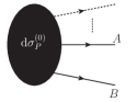
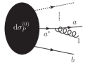
a) Original Configuration: $\mathrm{d}\sigma_{F}^{(0)}\hskip 1.79997pt$	b) A contribution to $\mathrm{d}\sigma_{F+1}^{(0)}\hskip 1.79997pt$	c) Recursion $\to$ $\mathrm{d}\sigma^{(0)}_{F+n}\hskip 1.79997pt$

Figure 9: a) and b) Illustration of the QCD singularities induced by on-shell propagators. c) The approximation obtained in the first step can be iterated to add additional legs.

the Feynman diagram in which parton “1” is emitted from the “$a$” (or “$b$”) leg has a pole for $s_{a1}\to 0$ ($s_{1b}\to 0$), corresponding to the intermediate propagator “$a^{*}$” (“$b^{*}$”) going on shell (middle pane). Summing the two and squaring them, i.e., including their mutual interference, one obtains the structure in equation (40), which is called the Eikonal factor.

The leading part of the singularity structure to which we have already referred many times is clearly visible here: if we integrate over the entire phase space including the region $s_{a1}\to 0$, $s_{1b}\to 0$, we end up with a double pole. If we instead regulate the divergence by cutting off the integration at some minimal perturbative cutoff scale $\mu_{\mathrm{IR}}^{2}$, we end up with a logarithm squared of that scale. This is a typical example of “large logs” being generated by the presence of scale hierarchies.

Before we continue, it is worth noting that equation (40) is often rewritten in other forms to emphasize specific aspects of it. One such rewriting is thus to reformulate the invariants $s_{i1}$ appearing in equation (40) in terms of energies and angles,

$$s_{ij}=2E_{i}E_{j}\left(1-\cos\theta_{ij}\right)~{}.$$ (41)

Rewritten in this way, the differentials in equation (40) become

$$\frac{\mathrm{d}s_{a1}\hskip 1.99997pt}{s_{a1}}\frac{\mathrm{d}s_{1b}\hskip 1.99997pt}{s_{1b}}\propto\frac{\mathrm{d}E_{1}\hskip 1.99997pt}{E_{1}}\frac{\mathrm{d}\theta_{a1}\hskip 1.99997pt}{\theta_{a1}}+\frac{\mathrm{d}E_{1}\hskip 1.99997pt}{E_{1}}\frac{\mathrm{d}\theta_{1b}\hskip 1.99997pt}{\theta_{1b}}~{}.$$ (42)

This kind of rewriting enables an intuitively appealing categorization of the singularities as related to vanishing energies and angles, called soft and collinear limits, respectively. Although such formulations have undeniably been helpful in obtaining many important results in QCD, one should still keep in mind that Lorentz non-invariant formulations come with similar caveats and warnings as do gauge non-invariant formulations of quantum field theory: while they can be practical to work with at intermediate stages of a calculation, one should be careful with any physical conclusions that rely explicitly on them. We shall therefore here restrict ourselves to a Lorentz invariant formalism based directly on equation (40). The collinear limit is then replaced by a more general single-pole limit in which a single parton-parton invariant vanishes (as, for instance, when a pair of partons become collinear), while the soft limit is replaced by one in which two (or more) invariants involving the same parton vanish simultaneously (as, for instance by that parton becoming soft in a frame defined by two or more hard partons). This avoids frame-dependent ambiguities from entering into the language, at the price of a slight reinterpretation of what is meant by collinear and soft.

Independently of rewritings and philosophy, the real power of equation (40) lies in the fact that it is universal. Thus, for any process $F$, we can apply equation (40) in order to get an approximation for $\mathrm{d}\sigma_{F+1}\hskip 1.99997pt$. We may then, for instance, take our newly obtained expression for $F+1$ as our arbitrary process and crank equation (40) again, to obtain an approximation for $\mathrm{d}\sigma_{F+2}\hskip 1.99997pt$, and so forth. What we have here is therefore a very simple recursion relation that can be used to generate approximations to leading-order cross sections with arbitrary numbers of additional legs. The quality of this approximation is governed by how many terms besides the leading one shown in equation (40) are included in the game. Including all possible terms, the most general form for the cross section at $F+n\,$ jets, restricted to the phase-space region above some infrared cutoff scale $\mu_{\mathrm{IR}}$, has the following algebraic structure,

$$\sigma_{F+n}^{(0)}=\alpha_{s}^{n}\left(\ln^{2n}+\ln^{2n-1}+\ln^{2n-2}+\ldots+\ln{}+{\cal R}\right)$$ (43)

where we use the notation $\ln^{\lambda}$ without an argument to denote generic functions of transcendentality $\lambda$ (the logarithmic function to the power $\lambda$ being a “typical” example of a function with transcendentality $\lambda$ appearing in cross section expressions, but also dilogarithms and higher logarithmic functions of transcendentality $>1$ should be implicitly understood to belong to our notation $\ln^{\lambda}$). The last term, $\cal R$, represents a rational function of transcendentality 0. We shall also use the nomenclature singular and finite for the $\ln^{\lambda}$ and ${\cal R}$ terms, respectively, a terminology which reflects their respective behaviour in the limit $\mu_{\mathrm{IR}}\to 0$.

The simplest approximation one can build on equation (43), dropping all but the leading $\ln^{2n}$ term in the parenthesis, is thus the leading-transcendentality approximation. This approximation is better known as the DLA (double logarithmic approximation), since it generates the correct coefficient for terms which have two powers of logarithms for each power of $\alpha_{s}$, while terms of lower transcendentalities are not guaranteed to have the correct coefficients. In so-called LL (leading-logarithmic) parton shower algorithms, one generally expects to reproduce the correct coefficients for the $\ln^{2n}$ and $\ln^{2n-1}$ terms. In addition, several formally subleading improvements are normally also introduced in such algorithms (such as explicit momentum conservation, gluon polarization and other spin-correlation effects [38], higher-order coherence effects, renormalization scale choices [39], finite-width effects [40], etc), as a means to improve the agreement with some of the more subleading coefficients as well, if not in every phase-space point then at least on average. Though LL showers do not magically acquire NLL (next-to-leading-log) precision from such procedures, one therefore still expects a significantly better average performance from them than from corresponding “strict” LL analytical resummations. A side effect of this is that it is often possible to “tune” shower algorithms to give better-than-nominal agreement with experimental distributions, by adjusting the parameters controlling the treatment of subleading effects. One should remember, however, that there is a limit to how much can be accomplished in this way — at some point, agreement with one process will only come at the price of disagreement with another, and at this point further tuning would be meaningless.

F @ LO$\times$LL(non-unitary)

$\ell$ (loops) 2   $\sigma^{(2)}_{0}$ $\sigma^{(2)}_{1}$ … 1   $\sigma^{(1)}_{0}$ $\sigma^{(1)}_{1}$ $\sigma^{(1)}_{2}$ … 0   $\sigma^{(0)}_{0}$ $\sigma^{(0)}_{1}$ $\sigma^{(0)}_{2}$ $\sigma^{(0)}_{3}$ … 0 1 2 3 … $k$ (legs)

F @ LO$\times$LL(unitary)

$\ell$ (loops) 2   $\sigma^{(2)}_{0}$ $\sigma^{(2)}_{1}$ … 1   $\sigma^{(1)}_{0}$ $\sigma^{(1)}_{1}$ $\sigma^{(1)}_{2}$ … 0   $\sigma^{(0)}_{0}$ $\sigma^{(0)}_{1}$ $\sigma^{(0)}_{2}$ $\sigma^{(0)}_{3}$ … 0 1 2 3 … $k$ (legs)

Figure 10: Coefficients of the perturbative series covered by LO + LL calculations, Left: without imposing unitarity, and Right: imposing unitarity order by order for each $n=k+\ell$. Green (darker) shading represents the full perturbative coefficient at the respective $k$ and $\ell$. Yellow (lighter) shading represents an LL approximation to it. Half-shaded boxes indicate phase spaces in which we are prohibited from integrating over the IR singular region, as discussed in sections 2.3 and 4.2.

Applying such an iterative process on a Born-level cross section, one obtains the description of the full perturbative series illustrated in the left-hand pane of figure 10. The yellow (lighter) shades used here for $k\geq 1$ indicate that the coefficient obtained is not the exact one, but rather an approximation to it that only gets its leading singularities right. However, since this is still only an approximation to infinite-order tree-level cross sections (we have not yet included any virtual corrections), we cannot yet integrate this approximation over all of phase space, as illustrated by the yellow boxes being only half filled on the left-hand side of figure 10; the summed total cross section would still be infinite. This particular approximation would therefore still appear to be very useless indeed — on one hand, it is only guaranteed to get the singular terms right, but on the other, it does not actually allow us to integrate over the singular region. In order to obtain a truly all-orders calculation, the constraint of unitarity must also be explicitly imposed, which furnishes an approximation to all-orders loop corrections as well. Let us therefore emphasize that figure 10 is included for pedagogical purposes only; all resummation calculations, whether analytical or parton-shower based, include virtual corrections as well and consequently yield finite total cross sections, as will now be described.

2.4.2 Step Two: Infinite Loops

Order-by-order unitarity, such as used in the KLN theorem, implies that the singularities caused by integration over unresolved radiation in the tree-level matrix elements must be canceled, order by order, by equal but opposite-sign singularities in the virtual corrections at the same order. That is, from equation (40), we immediately know that the 1-loop correction to $\mathrm{d}\sigma_{F}\hskip 1.99997pt$ must contain a term,

$$\mathrm{d}\sigma^{(1)}_{F}\hskip 1.99997pt=-g_{s}^{2}\,{\cal N}_{AB\to a1b}\,\mathrm{d}\sigma^{(0)}_{F}\hskip 1.99997pt\int\frac{\mathrm{d}s_{a1}\hskip 1.99997pt}{s_{a1}}\frac{\mathrm{d}s_{1b}\hskip 1.99997pt}{s_{1b}}~{}+~{}\mbox{less singular terms},$$ (44)

that cancels the divergence coming from equation (40) itself. Further, since this is universally true, we may apply equation (44) again to get an approximation to the corrections generated by equation (40) at the next order and so on. By adding such terms explicitly, order by order, we may now bootstrap our way around the entire perturbative series, using equation (40) to move horizontally and equation (44) to move along diagonals of constant $n=k+\ell$. Since real-virtual cancellations are now explicitly restored, we may finally extend the integrations over all of phase space, resulting in the picture shown on the right-hand pane of figure 10.

The right-hand pane, not the left-hand one, corresponds to what is actually done in resummation calculations, both of the analytic and parton-shower types. Physically, there is a significant and intuitive meaning to the imposition of unitarity, as follows.

Take a jet algorithm, with some measure of jet resolution, $Q$, and apply it to an arbitrary sample of events, say dijets. At a very crude resolution scale, corresponding to a high value for $Q$, you find that everything is clustered back to a dijet configuration, and the 2-jet cross section is equal to the total inclusive cross section,

$$\sigma_{\mathrm{tot}}=\sigma_{F;\mathrm{incl}}~{}.$$ (45)

At finer resolutions, decreasing $Q$, you see that some events that were previously classified as 2-jet events contain additional, lower-scale jets, that you can now resolve, and hence those events now migrate to the 3-jet bin, while the total inclusive cross section of course remains unchanged,

$$\sigma_{\mathrm{tot}}=\sigma_{F;\mathrm{incl}}=\sigma_{F;\mathrm{excl}}(Q)+\sigma_{F+1;\mathrm{incl}}(Q)~{},$$ (46)

where “incl” and “excl” stands for inclusive and exclusive cross sections, respectively, and the $Q$-dependence in the two terms on the right-hand side must cancel so that the total inclusive cross section is independent of $Q$. Later, some 3-jet events now migrate further, to 4 and higher jets, while still more 2-jet events migrate into the 3-jet bin, etc. For arbitrary $n$ and $Q$, we have

$$\sigma_{F+n;\mathrm{incl}}(Q)=\sigma_{F;\mathrm{incl}}-\sum_{m=0}^{n-1}\sigma_{F+m;\mathrm{excl}}(Q)~{}.$$ (47)

This equation expresses the trivial fact that the cross section for $n$ or more jets can be computed as the total inclusive cross section for $F$ minus a sum over the cross sections for $F$ + exactly $m$ jets including all $m<n$. On the theoretical side, it is these negative terms which must be included in the calculation, for each order $n=k+\ell$, to restore unitarity. Physically, they express that, at a given scale $Q$, a given event will be classified as having either 0, 1, 2, or whatever jets. Or, equivalently, for each event we gain in the 3-jet bin as $Q$ is lowered, we must loose one event in the 2-jet one; the negative contribution to the 2-jet bin is exactly minus the integral of the positive contribution to the 3-jet one, and so on. We may perceive of this detailed balance as an evolution of the event structure with $Q$, for each event, which is effectively what is done in parton-shower algorithms, to which we shall return in Section 4.1.

3 Soft QCD

In a complete high-energy collision, many different physics (sub-)processes contribute to the total observed activity. We here give a very brief overview of the main aspects of soft QCD that are relevant for hadron-hadron collisions, such as parton distribution functions, minimum-bias and soft-inclusive physics, and the so-called “underlying event”. This will be kept at a strictly pedestrian level and is largely based on the review in [41]. A discussion of the modeling of these components, as well as a discussion of the process of hadronization, is deferred to the relevant parts of Section 4 on Monte Carlo event generators.

3.1 Parton Densities

Physically, parton densities express the fact that hadrons are composite, with a time-dependent structure, illustrated in figure 11.

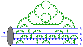
Figure 11: Illustration (from [42]) of partonic fluctuations inside a proton beam.

More formally, they are defined by the factorization theorem discussed in Section 2.1. Occasionally, the words structure functions and parton densities are used interchangeably. However, there is a very important distinction between the two, which we find often in (quantum) physics: one is a physical observable, the other is a “fundamental” quantity extracted from it.

Structure functions, such as $F_{2}$, are completely unambiguous physical observables, which can be measured, for instance, in DIS processes. (For a definition, see, e.g., [43].) From these, and other observables, a set of more fundamental and theoretically useful objects, parton density functions (PDFs), can be extracted, but there is a price; since the parton densities are not, themselves, physically observable, they can only be defined within a specific factorization scheme, order by order in perturbation theory. The only exception is at leading order, at which they have a very simple physical interpretation, as the probability of finding a quark of a given flavor and carrying a given momentum fraction, $x$, inside a hadron of a given type, probed at a specific scale, $Q^{2}$. They are then related to the structure function $F_{2}$ by their charge-weighted momentum sum,

$$\underbrace{F_{2}(x,Q^{2})}_{\mbox{\small Physical Observable}}=\sum_{i}e_{i}^{2}x\underbrace{f_{i}(x,Q^{2})}_{\mbox{\small Extracted Quantity}}~{},$$ (48)

where $f_{i}$ denotes the parton density for a parton of flavor/type $i$. When going to higher orders, we tend to keep the simple intuitive picture from leading order in mind, but one should be aware that the fundamental relationship is now more complicated, and that the parton densities no longer have a clear probabilistic interpretation.

The reader should also be aware that there is currently a significant amount of debate concerning many aspects of PDF definitions and usage:

• The “initial condition” for the PDFs, i.e., their shape in $x$ at some low value of $Q_{F}^{2}$, and other constraints imposed on their evolution, such as positivity, flavour symmetries, treatment of mass effects, and extrapolation beyond the fit region. Each PDF group has its own particular ideology when it comes to these issues, and while the differences caused by these choices in well-constrained regions may appear small, the user should be warned that large differences can occur when extrapolating, e.g., to small $x$, or for observables that are particularly sensitive, e.g., to flavour symmetries, etc.

• Using PDFs extracted using higher-order matrix elements in lower-order calculations, as, e.g., when using NLO PDFs as input to an LO calculation. In principle, the higher-order PDFs are better constrained and the difference between, e.g., an NLO and an LO set should formally be beyond LO precision, so that one might be tempted to simply use the highest-order available PDFs for any calculation. However, as described in section 2.4, it is often possible to partly absorb higher-order terms into lower-order coefficients. In the context of PDFs, the fit parameters of lower-order PDFs will effectively attempt to “compensate” for missing higher-order contributions in the matrix elements. To the extent those higher-order contributions are universal, this is both desirable and self-consistent. However, this will only give an improvement when used with matrix elements at the same order as those used to extract the PDFs. It is therefore quite possible that NLO PDFs used in conjunction with LO matrix elements give a worse agreement with data than LO PDFs do.

• PDF uncertainties. Uncertainty estimates for PDF determinations is a highly delicate procedure, owing in part to the diversity of the data sets that enter into the fitting procedures (especially since some data sets appear to have “tensions”, i.e., mutual incompatibilities, between them), but also the differences in philosophy mentioned above (e.g., on parametrizations and evolution constraints) can cause apparent incompatibilities between different sets which are hard to give precise uncertainty estimates for. Currently, a consensus on meaningful uncertainty estimates is slowly building, though future years are likely to see continued active discussions on how best to address this topic.

• How to use PDFs in conjunction with parton-shower Monte Carlo codes. The initial-state showers in a Monte Carlo model are essentially supposed to mimic the evolution in the PDFs, and vice versa. However, since PDF fits are not done with MC codes, but instead use analytical resummation models that are not identical to their MC counterparts, the PDF fits are essentially “tuned” to a slightly different resummation than that incorporated in a given MC model. Since both types of calculations are supposed to be accurate at least to LL, any difference between them should in principle be subleading. In practice, not much is known about the size and impact of this ambiguity, so we mention it mostly to make sure the reader is aware that it exists. Known differences include: the size of phase space (purely collinear massless PDF evolution vs. the finite-transverse-momentum massive MC phase space), the treatment of momentum conservation and recoil effects, additional higher-order effects explicitly or implicitly included in the MC evolution, choice of renormalization scheme and scale, and, for those MC algorithms that do not rely on collinear (DGLAP, see [22]) splitting kernels (e.g., the various kinds of dipole evolution algorithms, see [44]), differences in the effective factorization scheme.

3.2 Elastic and Inelastic Components of $\sigma_{\mathrm{tot}}$

Elastic scattering consists of all reactions of the type

$$A(p_{A})B(p_{B})\to A(p_{A}^{\prime})B(p_{B}^{\prime})~{},$$ (49)

where $A$ and $B$ are particles carrying momenta $p_{A}$ and $p_{B}$, respectively. Specifically, the only exchanged quantity is momentum; all quantum numbers and masses remain unaltered, and no new particles are produced. Inelastic scattering covers everything else, i.e.,

$$AB\to X\neq AB~{},$$ (50)

where $X\neq AB$ signifies that one or more quantum numbers are changed, and/or more particles are produced. The total hadron-hadron cross section can thus be written as a sum of these two physically distinguishable components,

$$\sigma_{\mathrm{tot}}(s)=\sigma_{\mathrm{el}}(s)+\sigma_{\mathrm{inel}}(s)~{},$$ (51)

where $s=(p_{A}+p_{B})^{2}$ is the beam-beam centre-of-mass energy squared.

If $A$ and/or $B$ are not elementary, the inelastic final states may be further divided into “diffractive” and “non-diffractive” topologies. This is a qualitative classification, usually based on whether the final state looks like the decay of an excitation of the beam particles (diffractive), or not (non-diffractive), or upon the presence of a large rapidity gap somewhere in the final state which would separate such excitations.

Given that an event has been labeled as diffractive, either within the context of a theoretical model, or by a final-state observable, we may distinguish between three different classes of diffractive topologies, which it is possible to distinguish between physically, at least in principle. In double-diffractive (DD) events, both of the beam particles are diffractively excited and hence none of them survive the collision intact. In single-diffractive (SD) events, only one of the beam particles gets excited and the other survives intact. The last diffractive topology is central diffraction (CD), in which both of the beam particles survive intact, leaving an excited system in the central region between them. (This latter topology includes “central exclusive production” where a single particle is produced in the central region.) That is,

$$\sigma_{\mathrm{inel}}(s)=\sigma_{\mathrm{SD}}(s)+\sigma_{\mathrm{DD}}(s)+\sigma_{\mathrm{CD}}(s)+\sigma_{\mathrm{ND}}(s)~{},$$ (52)

where “ND” (non-diffractive, here understood not to include elastic scattering) contains no gaps in the event consistent with the chosen definition of diffraction. Further, each of the diffractively excited systems in the events labeled SD, DD, and CD, respectively, may in principle consist of several subsystems with gaps between them. Eq. (52) may thus be defined to be exact, within a specific definition of diffraction, even in the presence of multi-gap events. Note, however, that different theoretical models almost always use different (model-dependent) definitions of diffraction, and therefore the individual components in one model are in general not directly comparable to those of another. It is therefore important that data be presented at the level of physical observables if unambiguous conclusions are to be drawn from them.

3.3 Minimum-bias and soft inclusive physics

The term “minimum-bias” (MB) is an experimental term, used to define a certain class of events that are selected with the minimum possible trigger bias, to ensure they are as inclusive as possible. In theoretical contexts, the term “minimum-bias” is often used with a slightly different meaning; to denote specific (classes of) inclusive soft-QCD subprocesses in a given model. Since these two usages are not exactly identical, in these lectures we have chosen to reserve the term “minimum bias” to pertain strictly to definitions of experimental measurements, and instead use the term “soft inclusive” physics as a generic descriptor for the class of processes which generally dominate the various experimental “minimum-bias” measurements in theoretical models. This parallels the terminology used in the review [41], from which most of the discussion here has been adapted. See equation (52) above for a compact overview of the types of physical processes that contribute to minimum-bias data samples. For a more detailed description of Monte Carlo models of this physics, in particular ones based on Multiple Parton Interactions (MPI), see Section 4.4.

3.4 Underlying event and jet pedestals

In events containing a hard parton-parton interaction, the underlying event (UE) can be roughly conceived of as the difference between QCD with and without including the remnants of the original beam hadrons. Without such “beam remnants”, only the hard interaction itself, and its associated parton showers and hadronization, would contribute to the observed particle production. In reality, after the partons that participate in the hard interaction have been taken out, the remnants still contain whatever is left of the incoming beam hadrons, including also a partonic substructure, which leads to the possibility of “multiple parton interactions” (MPI), as will be discussed in section 4.4. Due to the simple fact that the remnants are not empty, an “underlying event” will always be there — but how much additional energy does it deposit in a given measurement region? A quantifation of this can be obtained, for instance, by comparing measurements of the UE to the average activity in minimum-bias events at the same $\sqrt{s}$. Interestingly, it turns out that the underlying event is much more active, with larger fluctuations, than the average MB event. This is called the jet pedestal effect (hard jets sit on top of a higher-than-average “pedestal” of underlying activity), and is interpreted as follows. When two hadrons collide at non-zero impact parameter, high-$p_{\perp}$ interactions can only take place inside the overlapping region. Imposing a hard trigger therefore statistically biases the event sample toward more central collisions, which will also have more underlying activity. See Section 4.4 for a more detailed description of Monte Carlo models of this physics, based on MPI.

4 Monte Carlo Event Generators

In this section, we discuss the physics of Monte Carlo generators and their mathematical foundations, at an introductory level. We shall attempt to convey the main ideas as clearly as possible without burying them in an avalanche of technical details. References to more detailed discussions are included where applicable. We assume the reader is already familiar with the contents of the preceding sections of this report, in particular section 2.3 on matrix elements and section 2.4 on parton showers. Several of the discussions rely on material from the recent more comprehensive review in [41], which also contains brief descriptions of the physics implementations of each of the main general-purpose event generators on the market, together with a guide on how to use (and not use) generators in various connections, and a collection of comparisons to important experimental distributions. We highly recommend readers to obtain a copy of that review, as it is the most comprehensive and up-to-date review of event generators currently available. Another useful and pedagogical review on event generators is contained in the 2006 ESHEP lectures by Sjöstrand [42], with a more recent update in [45].

4.1 Perturbation Theory with Markov Chains

Consider again the Born-level cross section for an arbitrary hard process, $F$, differentially in an arbitrary infrared-safe observable $\cal O$, as obtained from equation (34):

$$\left.\frac{\mathrm{d}\sigma^{(0)}_{F}\hskip 1.99997pt}{\mathrm{d}\cal O\hskip 1.99997pt}\right|_{\mbox{{\color[rgb]{0,0,0}Born}}}=\int\mathrm{d}\Phi_{F}\hskip 1.99997pt\ |{\cal M}_{F}^{(0)}|^{2}\ \delta({\cal O}-{\cal O}(\Phi_{F}))~{},$$ (53)

where the integration runs over the full final-state on-shell phase space of $F$ (this expression and those below would also apply to hadron collisions were we to include integrations over the parton distribution functions in the initial state), and the $\delta$ function projects out a 1-dimensional slice defined by $\cal O$ evaluated on the set of final-state momenta which we denote $\Phi_{F}$.

To make the connection to parton showers, we insert an operator, ${\cal S}$, that acts on the Born-level final state before the observable is evaluated, i.e.,

$$\left.\frac{\mathrm{d}\sigma_{F}\hskip 1.99997pt}{\mathrm{d}\cal O\hskip 1.99997pt}\right|_{\mbox{{\color[rgb]{0,0,0}${\cal S}$}}}=\int\mathrm{d}\Phi_{F}\hskip 1.99997pt\ |{\cal M}_{F}^{(0)}|^{2}\ {\cal S}(\Phi_{F},{\cal O})~{}.$$ (54)

Formally, this operator — the evolution operator — will be responsible for generating all (real and virtual) higher-order corrections to the Born-level expression. The measurement $\delta$ function appearing explicitly in equation (53) is now implicit in ${\cal S}$.

Algorithmically, parton showers cast $\cal S$ as an iterative Markov (i.e., history-independent) chain, with an evolution parameter, $Q_{E}$, that formally represents the factorization scale of the event, below which all structure is summed over inclusively. Depending on the particular choice of shower algorithm, $Q_{E}$ may be defined as a parton virtuality (virtuality-order showers), as a transverse-momentum scale ($p_{\perp}$-ordered showers), or as a combination of energies times angles (angular ordering). Regardless of the specific form of $Q_{E}$, the evolution parameter will go towards zero as the Markov chain develops, and the event structure will become more and more exclusively resolved. A transition from a perturbative evolution to a non-perturbative one can also be inserted, when the evolution reaches an appropriate scale, typically around $1$ GeV. This scale thus represents the lowest perturbative scale that can appear in the calculations, with all perturbative corrections below it summed over inclusively.

Working out the precise form that $\cal S$ must have in order to give the correct expansions discussed in section 2.4 takes a bit of algebra, and is beyond the scope we aim to cover in these lectures. Heuristically, the procedure is as follows. We noted that the singularity structure of QCD is universal and that at least its first few terms are known to us. We also saw that we could iterate that singularity structure, using universality and unitarity, thereby bootstrapping our way around the entire perturbative series. This was illustrated by the right-hand pane of figure 10 in section 2.4.

Skipping intermediate steps, the form of the all-orders pure-shower Markov chain, for the evolution of an event between two scales $Q_{E1}>Q_{E2}$, is,

$$\begin{array}[]{rcl}\displaystyle{\cal S}(\Phi_{F},Q_{E1},Q_{E2},\mathcal{O})&=&\displaystyle\underbrace{\Delta(\Phi_{F},Q_{E1},Q_{E2})\ \delta\left(\mathcal{O}-\mathcal{O}(\Phi_{F})\right)}_{\mbox{$F+0$ exclusive above $Q_{E2}$}}\\[25.60747pt] &&+\displaystyle\underbrace{\sum_{r}\int_{Q_{E2}}^{Q_{E1}}\frac{\mathrm{d}\Phi_{F+1}^{r}\hskip 1.99997pt}{\mathrm{d}\Phi_{F}\hskip 1.99997pt}\ S_{r}(\Phi_{F+1})\ \Delta(\Phi_{F},Q_{E1},Q_{F+1})\ {\cal S}(\Phi_{F+1},Q_{F+1},Q_{E2},\mathcal{O})}_{\mbox{$F+1$ inclusive above $Q_{E2}$}}~{},\end{array}$$ (55)

with the so-called Sudakov factor,

$$\Delta(\Phi_{F},Q_{E1},Q_{E2})=\exp\left[-\sum_{r}\int_{Q_{E2}}^{Q_{E1}}\frac{\mathrm{d}\Phi_{F+1}^{r}\hskip 1.99997pt}{\mathrm{d}\Phi_{F}\hskip 1.99997pt}S_{r}(\Phi_{F+1})\right]~{},$$ (56)

defining the probability that there is no evolution (i.e., no emissions) between the scales $Q_{E1}$ and $Q_{E2}$, according to the radiation functions $S_{r}$ to which we shall return below. The term on the first line of equation (55) thus represents all events that did not evolve as the resolution scale was lowered from $Q_{E1}$ to $Q_{E2}$, while the second line contains a sum and phase-space integral over those events that did evolve — including the insertion of ${\cal S}(\Phi_{F+1})$ representing the possible further evolution of the event and completing the iterative definition of the Markov chain.

The factor $\mathrm{d}\Phi_{F+1}^{r}\hskip 1.99997pt/\mathrm{d}\Phi_{F}\hskip 1.99997pt$ defines the chosen phase space factorization. Our favourite is the so-called dipole-antenna factorization, whose principal virtue is that it is the simplest Lorentz invariant factorization which is simultaneously exact over all of phase space while only involving on-shell momenta. For completeness, its form is

$$\frac{\mathrm{d}\Phi_{F+1}^{r}\hskip 1.99997pt}{\mathrm{d}\Phi_{F}\hskip 1.99997pt}=\frac{\mathrm{d}\Phi_{3}^{r}\hskip 1.99997pt}{\mathrm{d}\Phi_{2}\hskip 1.99997pt}=\mathrm{d}s_{a1}\hskip 1.99997pt\mathrm{d}s_{1b}\hskip 1.99997pt\frac{\mathrm{d}\phi\hskip 1.99997pt}{2\pi}\frac{1}{16\pi^{2}s_{r}}~{},$$ (57)

which involves just one colour-anticolour pair for each $r$, with invariant mass squared $s_{r}=(p_{a}+p_{1}+p_{b})^{2}$. Other choices, such as purely collinear ones (only exact in the collinear limit or involving explicitly off-shell momenta), more global ones involving all partons in the event (more complicated, in our opinion), or less global ones with a single parton playing the dominant role as emitter, are also possible, again depending on the specific algorithm considered.

The radiation functions $S_{r}$ obviously play a crucial role in these equations, driving the emission probabilities. For example, if $S_{r}\to 0$, then $\Delta\to\exp(0)=1$ and all events stay in the top line of equation (55). Thus, in regions of phase space where $S_{r}$ is small, there is little or no evolution. Conversely, for $S_{r}\to\infty$, we have $\Delta\to 0$, implying that all events evolve. One possible choice for the radiation functions $S_{r}$ was implicit in equation (40), in which we took them to include only the leading (double) singularities, with $r$ representing colour-anticolour pairs. In general, the shower may exponentiate the entire set of universal singular terms, or only a subset of them (for example, the terms leading in the number of colours $N_{C}$), which is why we here let the explicit form of $S_{r}$ be unspecified. Suffice it to say that in traditional parton showers, $S_{r}$ would simply be the DGLAP splitting kernels (see, e.g., [22]), while they would be so-called dipole or antenna radiation functions in the various dipole-based approaches to QCD (see, e.g., [46, 47, 48, 49, 34, 35]).

The procedure for how to technically “construct” a shower algorithm of this kind, using random numbers to generate scales distributed according to equation (55), is described more fully in [34], using a notation that closely parallels the one used here. The procedure is also described at a more technical level in the review [41], though using a slightly different notation. Finally, a pedagogical introduction to Monte Carlo methods in general can be found in [29].

4.2 Matching

The essential problem that leads to matrix-element/parton-shower matching can be illustrated in a very simple way.

F @ LO$\times$LL

$\ell$ (loops) 2   $\sigma^{(2)}_{0}$ $\sigma^{(2)}_{1}$ … 1   $\sigma^{(1)}_{0}$ $\sigma^{(1)}_{1}$ $\sigma^{(1)}_{2}$ … 0   $\sigma^{(0)}_{0}$ $\sigma^{(0)}_{1}$ $\sigma^{(0)}_{2}$ $\sigma^{(0)}_{3}$ … 0 1 2 3 … $k$ (legs)

+ F+1 @ LO$\times$LL    $\ell$ (loops) 2   $\sigma^{(2)}_{0}$ $\sigma^{(2)}_{1}$ … 1   $\sigma^{(1)}_{0}$ $\sigma^{(1)}_{1}$ $\sigma^{(1)}_{2}$ … 0   $\sigma^{(0)}_{0}$ $\sigma^{(0)}_{1}$ $\sigma^{(0)}_{2}$ $\sigma^{(0)}_{3}$ … 0 1 2 3 … $k$ (legs) = F & F+1 @ LO$\times$LL    $\ell$ (loops) 2   $\sigma^{(2)}_{0}$ $\sigma^{(2)}_{1}$ … 1   $\sigma^{(1)}_{0}$ $\sigma^{(1)}_{1}$ $\sigma^{(1)}_{2}$ … 0   $\sigma^{(0)}_{0}$ $\sigma^{(0)}_{1}$ $\sigma^{(0)}_{2}$ $\sigma^{(0)}_{3}$ … 0 1 2 3 … $k$ (legs)

Figure 12: Illustration of the double-counting problem caused by naively adding cross sections involving matrix elements with different numbers of legs.

Assume we have computed the LO cross section for some process, $F$, and that we have added an LL shower to it, as in the left-hand pane of figure 12. We know that this only gives us an LL description of $F+1$. We now wish to improve this from LL to LO by adding the actual LO matrix element for $F+1$. Since we also want to be able to hadronize these events, etc, we again add an LL shower off them. However, since the matrix element for $F+1$ is divergent, we must restrict it to cover only the phase-space region with at least one hard resolved jet, illustrated by the half-shaded boxes in the middle pane of figure 12. Adding these two samples, however, we end up counting the LL terms of the inclusive cross section for $F+1$ twice, since we are now getting them once from the shower off $F$ and once from the matrix element for $F+1$, illustrated by the dark shaded (red) areas of the right-hand pane of figure 12. This double-counting problem would grow worse if we attempted to add more matrix elements, with more legs. The cause is very simple. Each such calculation corresponds to an inclusive cross section, and hence naive addition would give

$$\sigma_{\mathrm{tot}}=\sigma_{0;\mathrm{incl}}+\sigma_{1;\mathrm{incl}}=\sigma_{0;\mathrm{excl}}+2\,\sigma_{1;\mathrm{incl}}~{}.$$ (58)

Instead, we must match the coefficients calculated by the two parts of the full calculation — showers and matrix elements — more systematically, for each order in perturbation theory, so that the nesting of inclusive and exclusive cross sections is respected without overcounting.

Given a parton shower and a matrix-element generator, there are fundamentally three different ways in which we can consider matching the two [34]:

1. Slicing: The most commonly encountered matching type is currently based on separating (slicing) phase space into two regions, one of which is supposed to be mainly described by hard matrix elements and the other of which is supposed to be described by the shower. This type of approach was first used in Herwig [50], to include matrix-element corrections for one emission beyond the basic hard process [51, 52]. This is illustrated in figure 13.

F @ LO$\times$LL-Soft (Herwig Shower)

$\ell$ (loops) 2   $\sigma^{(2)}_{0}$ $\sigma^{(2)}_{1}$ … 1   $\sigma^{(1)}_{0}$ $\sigma^{(1)}_{1}$ $\sigma^{(1)}_{2}$ … 0   $\sigma^{(0)}_{0}$ $\sigma^{(0)}_{1}$ $\sigma^{(0)}_{2}$ $\sigma^{(0)}_{3}$ … 0 1 2 3 … $k$ (legs)

+ F+1 @ LO$\times$LL (Herwig Corrections)    $\ell$ (loops) 2   $\sigma^{(2)}_{0}$ $\sigma^{(2)}_{1}$ … 1   $\sigma^{(1)}_{0}$ $\sigma^{(1)}_{1}$ $\sigma^{(1)}_{2}$ … 0   $\sigma^{(0)}_{0}$ $\sigma^{(0)}_{1}$ $\sigma^{(0)}_{2}$ $\sigma^{(0)}_{3}$ … 0 1 2 3 … $k$ (legs) = F @ LO${}_{1}\times$LL (Herwig Matched)    $\ell$ (loops) 2   $\sigma^{(2)}_{0}$ $\sigma^{(2)}_{1}$ … 1   $\sigma^{(1)}_{0}$ $\sigma^{(1)}_{1}$ $\sigma^{(1)}_{2}$ … 0   $\sigma^{(0)}_{0}$ $\sigma^{(0)}_{1}$ $\sigma^{(0)}_{2}$ $\sigma^{(0)}_{3}$ … 0 1 2 3 … $k$ (legs)

Figure 13: Illustration of the original matching scheme implemented in Herwig [51, 52], in which the dead zone of the Herwig shower was used as an effective “matching scale” for one emission beyond a basic hard process.

The method has since been generalized by several independent groups to include arbitrary numbers of additional legs [53, 54, 55, 56, 57]. Effectively, the shower approximation is set to zero above some scale (either due to the presence of explicit dead zones in the shower, as in Herwig, or by vetoing any emissions above a certain matching scale, as in the (L)-CKKW [53, 54, 56] and MLM [57, 55] approaches), causing the matched result to be identical to the matrix element (ME) in that region, modulo higher-order corrections. We may sketch this as

$$\mbox{Matched (above matching scale)}=\color[rgb]{0.5,0.5,0.5}\overbrace{\color[rgb]{0,0,0}\mbox{Exact}}^{\small\mbox{ME}}~{}\ {\color[rgb]{0,0,0}\times}\ \overbrace{\color[rgb]{0,0,0}(1+\mathcal{O}(\alpha_{s}))}^{\small\mbox{corrections}}~{},$$ (59)

where the “shower-corrections” include approximate Sudakov factors and $\alpha_{s}$ reweighting factors applied to the matrix elements in order to obtain a smooth transition to the shower-dominated region. Below the matching scale, the small difference between the matrix elements and the shower approximation can be dropped (since their leading singularities are identical and this region by definition includes no hard jets), yielding the pure shower answer in that region,

Matched (below matching scale) $$= \color[rgb]{0.5,0.5,0.5}\overbrace{\color[rgb]{0,0,0}\mbox{Approximate}}^{\mbox{shower}}\ {\color[rgb]{0,0,0}+}\ \overbrace{\color[rgb]{0,0,0}(\mbox{Exact}-\mbox{Approximate})}^{\mbox{correction}}$$ (60)

$$= \mbox{Approximate}\ +\ \mbox{non-singular}$$

$$\to \mbox{Approximate}~{}.$$

This type of strategy is illustrated in figure 14.

F @ LO$\times$LL-Soft (excl)

$\ell$ (loops) 2   $\sigma^{(2)}_{0}$ … 1   $\sigma^{(1)}_{0}$ $\sigma^{(1)}_{1}$ … 0   $\sigma^{(0)}_{0}$ $\sigma^{(0)}_{1}$ $\sigma^{(0)}_{2}$ 0 1 2 $k$ (legs)

+ F+1 @ LO$\times$LL-Soft (excl)    $\ell$ (loops) 2   $\sigma^{(2)}_{0}$ … 1   $\sigma^{(1)}_{0}$ $\sigma^{(1)}_{1}$ … 0   $\sigma^{(0)}_{0}$ $\sigma^{(0)}_{1}$ $\sigma^{(0)}_{2}$ 0 1 2 $k$ (legs) + F+2 @ LO$\times$LL (incl)    $\ell$ (loops) 2   $\sigma^{(2)}_{0}$ … 1   $\sigma^{(1)}_{0}$ $\sigma^{(1)}_{1}$ … 0   $\sigma^{(0)}_{0}$ $\sigma^{(0)}_{1}$ $\sigma^{(0)}_{2}$ 0 1 2 $k$ (legs) = F @ LO${}_{2}\times$LL (MLM & (L)-CKKW)    $\ell$ (loops) 2   $\sigma^{(2)}_{0}$ … 1   $\sigma^{(1)}_{0}$ $\sigma^{(1)}_{1}$ … 0   $\sigma^{(0)}_{0}$ $\sigma^{(0)}_{1}$ $\sigma^{(0)}_{2}$ 0 1 2 $k$ (legs)

Figure 14: Illustration of slicing approaches to matching, with up to two additional emissions beyond the basic process. The showers off $F$ and $F+1$ are set to zero above a specific “matching scale”. (The number of coefficients shown was reduced a bit in these plots to make them fit in one row.)

Since this strategy is discontinuous across phase space, a main point here is to ensure that the behaviour across the matching scale be as smooth as possible. CKKW showed [53] that it is possible to remove any dependence on the matching scale through NLL precision by careful choices of all ingredients in the matching; technical details of the implementation (affecting the $\mathcal{O}(\alpha_{s})$ terms in eq. (59)) are important, and the dependence on the unphysical matching scale may be larger than NLL unless the implementation matches the theoretical algorithm precisely [54, 56, 58]. One should also be aware that all strategies of this type are quite computing intensive. This is basically due to the fact that a separate phase-space generator is required for each of the $n$-parton correction terms, with each such sample a priori consisting of weighted events such that a separate unweighting step (often with quite low efficiency) is needed before an unweighted sample can be produced.

2. Subtraction: Another way of matching two calculations is by subtracting one from the other and correcting by the difference, schematically

$$\mbox{Matched}=\color[rgb]{0.5,0.5,0.5}\overbrace{\color[rgb]{0,0,0}\mbox{Approximate}}^{\mbox{shower}}\color[rgb]{0,0,0}\ +\ \color[rgb]{0.5,0.5,0.5}\overbrace{\color[rgb]{0,0,0}(\mbox{Exact}-\mbox{Approximate})}^{\mbox{correction}}~{}.$$ (61)

This looks very much like the structure of an NLO fixed-order calculation, in which the shower approximation plays the role of subtraction terms, and indeed this is what is used in strategies like Mc@nlo [59, 60, 61], illustrated in figure 15.

F @ LO$\times$LL

$\ell$ (loops) 2   $\sigma^{(2)}_{0}$ $\sigma^{(2)}_{1}$ … 1   $\sigma^{(1)}_{0}$ $\sigma^{(1)}_{1}$ $\sigma^{(1)}_{2}$ … 0   $\sigma^{(0)}_{0}$ $\sigma^{(0)}_{1}$ $\sigma^{(0)}_{2}$ $\sigma^{(0)}_{3}$ … 0 1 2 3 … $k$ (legs)

+ (F @ NLO$\times$LL) - (F @ LO$\times$LL)    $\ell$ (loops) 2   $\sigma^{(2)}_{0}$ $\sigma^{(2)}_{1}$ … 1   $\sigma^{(1)}_{0}$ $\sigma^{(1)}_{1}$ $\sigma^{(1)}_{2}$ … 0   $\sigma^{(0)}_{0}$ $\sigma^{(0)}_{1}$ $\sigma^{(0)}_{2}$ $\sigma^{(0)}_{3}$ … 0 1 2 3 … $k$ (legs) = F @ NLO$\times$LL (Mc@nlo)    $\ell$ (loops) 2   $\sigma^{(2)}_{0}$ $\sigma^{(2)}_{1}$ … 1   $\sigma^{(1)}_{0}$ $\sigma^{(1)}_{1}$ $\sigma^{(1)}_{2}$ … 0   $\sigma^{(0)}_{0}$ $\sigma^{(0)}_{1}$ $\sigma^{(0)}_{2}$ $\sigma^{(0)}_{3}$ … 0 1 2 3 … $k$ (legs)

Figure 15: Illustration of the Mc@nlo approach to matching. In the middle pane, cyan boxes denote non-singular correction terms, while the egg-coloured ones denote showers off such corrections, which cannot lead to double-counting at the LL level.

In this type of approach, however, negative-weight events will generally occur, for instance in phase-space points where the approximation is larger than the exact answer. This motivated the development of the so-called Powheg approach [62], illustrated in figure 16,

F @ LO${}_{1}\times$LL

$\ell$ (loops) 2   $\sigma^{(2)}_{0}$ $\sigma^{(2)}_{1}$ … 1   $\sigma^{(1)}_{0}$ $\sigma^{(1)}_{1}$ $\sigma^{(1)}_{2}$ … 0   $\sigma^{(0)}_{0}$ $\sigma^{(0)}_{1}$ $\sigma^{(0)}_{2}$ $\sigma^{(0)}_{3}$ … 0 1 2 3 … $k$ (legs)

+ (F @ NLO$\times$LL) - (F @ LO${}_{1}\times$LL)    $\ell$ (loops) 2   $\sigma^{(2)}_{0}$ $\sigma^{(2)}_{1}$ … 1   $\sigma^{(1)}_{0}$ $\sigma^{(1)}_{1}$ $\sigma^{(1)}_{2}$ … 0   $\sigma^{(0)}_{0}$ $\sigma^{(0)}_{1}$ $\sigma^{(0)}_{2}$ $\sigma^{(0)}_{3}$ … 0 1 2 3 … $k$ (legs) = F @ NLO$\times$LL (Powheg)    $\ell$ (loops) 2   $\sigma^{(2)}_{0}$ $\sigma^{(2)}_{1}$ … 1   $\sigma^{(1)}_{0}$ $\sigma^{(1)}_{1}$ $\sigma^{(1)}_{2}$ … 0   $\sigma^{(0)}_{0}$ $\sigma^{(0)}_{1}$ $\sigma^{(0)}_{2}$ $\sigma^{(0)}_{3}$ … 0 1 2 3 … $k$ (legs)

Figure 16: Illustration of the Powheg approach to matching. In the middle pane, cyan boxes denote non-singular correction terms, while the egg-coloured ones denote showers off such corrections, which cannot lead to double-counting at the LL level.

which is constructed specifically to prevent negative-weight events from occurring and simultaneously to be more independent of which parton-shower algorithm it is used with. The advantage of these methods is obviously that NLO corrections to the Born level can be systematically incorporated. However, a systematic way of extending this strategy beyond the first additional emission is not available, save for combining them with a slicing-based strategy for the additional legs, as in Menlops [63], illustrated in figure 17.

F @ NLO$\times$LL-Soft ($\sim$ Powheg)

$\ell$ (loops) 2   $\sigma^{(2)}_{0}$ $\sigma^{(2)}_{1}$ … 1   $\sigma^{(1)}_{0}$ $\sigma^{(1)}_{1}$ $\sigma^{(1)}_{2}$ … 0   $\sigma^{(0)}_{0}$ $\sigma^{(0)}_{1}$ $\sigma^{(0)}_{2}$ $\sigma^{(0)}_{3}$ … 0 1 2 3 … $k$ (legs)

+ F +2 @ LO${}_{n}\times$LL ($\sim$ CKKW for F+2)    $\ell$ (loops) 2   $\sigma^{(2)}_{0}$ $\sigma^{(2)}_{1}$ … 1   $\sigma^{(1)}_{0}$ $\sigma^{(1)}_{1}$ $\sigma^{(1)}_{2}$ … 0   $\sigma^{(0)}_{0}$ $\sigma^{(0)}_{1}$ $\sigma^{(0)}_{2}$ $\sigma^{(0)}_{3}$ … 0 1 2 3 … $k$ (legs) = F @ NLO$\times$LL (Menlops)    $\ell$ (loops) 2   $\sigma^{(2)}_{0}$ $\sigma^{(2)}_{1}$ … 1   $\sigma^{(1)}_{0}$ $\sigma^{(1)}_{1}$ $\sigma^{(1)}_{2}$ … 0   $\sigma^{(0)}_{0}$ $\sigma^{(0)}_{1}$ $\sigma^{(0)}_{2}$ $\sigma^{(0)}_{3}$ … 0 1 2 3 … $k$ (legs)

Figure 17: Illustration of the Menlops approach to matching. Note that each of the Powheg and CKKW samples are composed of separate sub-samples, as illustrated in figures 14 and 16.

These issues are, however, no more severe than in ordinary fixed-order NLO approaches, and hence they are not viewed as disadvantages if the point of reference is an NLO computation.

3. Unitarity: The oldest, and in our view most attractive, approach [64, 65] consists of working out the shower approximation to a given fixed order, and correcting the shower splitting functions at that order by a multiplicative factor given by the ratio of the matrix element to the shower approximation, phase-space point by phase-space point. We may sketch this as

$$\mbox{Matched}=\color[rgb]{0.5,0.5,0.5}\overbrace{\color[rgb]{0,0,0}\mbox{Approximate}}^{\mbox{shower}}\ {\color[rgb]{0,0,0}\times}\ \overbrace{\color[rgb]{0,0,0}\frac{\mbox{Exact}}{\mbox{Approximate}}}^{\mbox{correction}}~{}.$$ (62)

When these correction factors are inserted back into the shower evolution, they guarantee that the shower evolution off $n-1$ partons correctly reproduces the $n$-parton matrix elements, without the need to generate a separate $n$-parton sample. That is, the shower approximation is essentially used as a pre-weighted (stratified) all-orders phase-space generator, on which a more exact answer can subsequently be imprinted order by order in perturbation theory. In the original approach [64, 65], used by Pythia [66, 67], this was only worked out for one additional emission beyond the basic hard process. In Powheg [62], it was extended to include also virtual corrections to the Born-level matrix element. Finally, in Vincia [34], it has been extended to include arbitrary numbers of emissions at tree level, though that method has so far only been applied to final-state showers.

F @ LO1+LL (Pythia)

$\ell$ (loops) 2   $\sigma^{(2)}_{0}$ $\sigma^{(2)}_{1}$ … 1   $\sigma^{(1)}_{0}$ $\sigma^{(1)}_{1}$ $\sigma^{(1)}_{2}$ … 0   $\sigma^{(0)}_{0}$ $\sigma^{(0)}_{1}$ $\sigma^{(0)}_{2}$ $\sigma^{(0)}_{3}$ … 0 1 2 3 … $k$ (legs)

F @ NLO+LOn+LL (Vincia)

$\ell$ (loops) 2   $\sigma^{(2)}_{0}$ $\sigma^{(2)}_{1}$ … 1   $\sigma^{(1)}_{0}$ $\sigma^{(1)}_{1}$ $\sigma^{(1)}_{2}$ … 0   $\sigma^{(0)}_{0}$ $\sigma^{(0)}_{1}$ $\sigma^{(0)}_{2}$ $\sigma^{(0)}_{3}$ … 0 1 2 3 … $k$ (legs)

Figure 18: Illustration of the two purely unitarity-based approaches to matching discussed in the text. Only one event sample is produced by each of these methods, and hence no sub-components are shown.

An illustration of the perturbative coefficients that can be included in each of these approaches is illustrated in figure 18, as usual with green (darker shaded) boxes representing exact coefficients and yellow (light shaded) boxes representing logarithmic approximations. Finally, two more properties unique to this method deserve mention. Firstly, since the corrections modify the actual shower evolution kernels, the corrections are automatically resummed in the Sudakov exponential, which should improve the logarithmic precision once $k\geq 2$ is included, and secondly, since the shower is unitary, an initially unweighted sample of $(n-1)$-parton configurations remains unweighted, with no need for a separate event-unweighting or event-rejection step.

4.3 The String Model of Hadronization

In the context of event generators, hadronization denotes the process by which a set of post-shower partons is transformed into a set of primary hadrons, which may then subsequently decay further. This non-perturbative transition takes place at the hadronization scale, which by construction is identical to the infrared cutoff of the parton shower. In the absence of a first-principles solution to the relevant dynamics, event generators use QCD-inspired phenomenological models to describe this transition.

Although non-perturbative QCD is not solved, we do have some knowledge of the properties that such a solution must have. For instance, Poincaré invariance, unitarity, and causality are all concepts that apply beyond perturbation theory. In addition, lattice QCD provides us a means of making explicit quantitative studies in a genuinely non-perturbative setting, albeit only of certain questions.

An important result in “quenched” lattice QCD is that the potential of the colour dipole field between a charge and an anticharge appears to grow linearly with the separation of the charges, when the separation is greater than about a femtometer.This is known as “linear confinement”, and it forms the starting point for the string model of hadronization.

Starting from early concepts developed by Artru and Mennessier [68], several hadronization models based on strings were proposed in the late 1970’ies and early 80’ies. Of these, the most sophisticated and widely used today is the so-called Lund model, implemented in the Pythia code. We shall therefore concentrate on that particular model here, though many of the overall concepts would be shared by any string-inspired method. (A more extended discussion can be found in the very complete and pedagogical review of the Lund model by Andersson [69].)

Consider the production of a $q\bar{q}$ pair from vacuum, for instance in the process $e^{+}e^{-}\to\gamma^{*}/Z\to q\bar{q}\to\mbox{hadrons}$. As the quarks move apart, linear confinement implies that a potential

$$V(r)=\kappa\,r$$ (63)

is asymptotically reached for large distances, $r$. (At short distances, there is a Coulomb term proportional to $1/r$ as well, but this is neglected in the Lund model.) This potential describes a string with tension (energy per unit length) $\kappa$. The physical picture is that of a colour flux tube being stretched between the $q$ and the $\bar{q}$, figure 19.

$1\,$fm

Figure 19: Illustration of the transition between a Coulomb potential at short distances to the string-like one of equation (63) at large $q\bar{q}$ separations.

From hadron mass spectroscopy the string tension $\kappa$, is known to be

$$\kappa~{}\sim~{}1\,\mbox{GeV/fm}~{}\sim~{}0.2\,\mbox{GeV}^{2}.$$ (64)

A straightforward Lorentz-invariant description of this object is provided by the massless relativistic string in 1+1 dimensions, with no transverse degrees of freedom. The mathematical, one-dimensional string can be thought of as parameterizing the position of the axis of a cylindrically symmetric flux tube. (Note that the expression “massless” is somewhat of a misnomer, since $\kappa$ effectively corresponds to a “mass density” along the string.)

As the $q$ and $\bar{q}$ move apart, their kinetic energy is gradually converted to potential energy, stored in the growing string spanned between them. In the “quenched” approximation, in which $g\to q\bar{q}$ splittings are not allowed, this process would continue until the endpoint quarks have lost all their momentum, at which point they would reverse direction and be accelerated by the now shrinking string. In the real world, quark-antiquark fluctuations inside the string field can make the transition to become real particles by absorbing energy from the string, thereby screening the original endpoint charges from each other and breaking the string into two separate colour-singlet pieces, $(q\bar{q})\to(q\bar{q}^{\prime})+(q^{\prime}\bar{q})$, illustrated in figure 20 ​a.

	time space
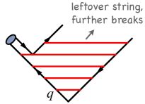
a)		b)

Figure 20: a) Illustration of string breaking by quark pair creation in the string field. b) Illustration of the algorithmic choice to process the fragmentation from the outside-in, splitting off a single on-shell hadron in each step.

This process then continues until only ordinary hadrons remain. (We will give more details on the individual string breaks below.) More complicated multi-parton topologies including gluons are treated by representing gluons as transverse “kinks”. Thus soft gluons effectively “build up” a transverse structure in the originally one-dimensional object, with infinitely soft ones absorbed into the string without leading to modifications. For strings with finite-energy kinks, the space-time evolution is then slightly more involved [69], and modifications to the fragmentation model to handle stepping across gluon corners have to be included, but the main point is that there are no separate free parameters for gluon jets. Differences with respect to quark fragmentation arise simply because quarks are only connected to a single string piece, while gluons have one on either side, increasing the energy loss per unit (invariant) time from a gluon to the string by a factor of 2 relative to quarks, which can be compared to the ratio of colour Casimirs $C_{A}/C_{F}=2.25$.

Since the string breaks are causally disconnected (as can easily be realized from space-time diagrams [69]), they do not have to be considered in any specific time-ordered sequence. In the Lund model, the string breaks are instead generated starting with the leading hadrons, containing the endpoint quarks, and iterating inwards towards the centre of the string, alternating randomly between fragmentation off the left- and right-hand sides, respectively, figure 20 ​b. This has the advantage that a single on-shell hadron can be split off in each step, making it straightforward to ensure that only states consistent with the known spectrum of hadron resonances are produced, as will be discussed below.

The details of the individual string breaks are not known from first principles. The Lund model invokes the idea of quantum mechanical tunneling, which leads to a Gaussian suppression of the energies and masses imparted to the produced quarks,

$$\mathrm{Prob}(m_{q}^{2},p_{\perp q}^{2})~{}\propto~{}\exp\left(\frac{-\pi m_{q}^{2}}{\kappa}\right)\exp\left(\frac{-\pi p_{\perp q}^{2}}{\kappa}\right)~{},$$ (65)

where $m_{q}$ is the mass of the produced quark and $p_{\perp}$ is the transverse momentum imparted to it by the breakup process (the antiquark obviously has the same mass and opposite $p_{\perp}$).

Due to the factorization of the $p_{\perp}$and $m$ dependence implied by equation (65), the $p_{\perp}$spectrum of produced quarks in this model is independent of the quark flavour, with a universal average value of

$$\left<p_{\perp q}^{2}\right>=\sigma^{2}=\kappa/\pi\sim(250\,\mbox{MeV})^{2}~{}.$$ (66)

Bear in mind that “transverse” is here defined with respect to the string axis. Thus, the $p_{\perp}$in a frame where the string is moving is modified by a Lorentz boost factor. Also bear in mind that $\sigma^{2}$ is here a purely non-perturbative parameter. In a Monte Carlo model with a fixed shower cutoff, the effective amount of “non-perturbative” $p_{\perp}$may be larger than this, due to effects of additional unresolved soft-gluon radiation below the shower cutoff scale. In principle, the magnitude of this additional component should scale with the cutoff, but in practice it is up to the user to enforce this by retuning the effective $\sigma$ parameter when changing the hadronization scale. Since hadrons receive $p_{\perp}$ contributions from two breakups, one on either side, their average transverse momentum squared will be twice as large,

$$\left<p_{\perp h}^{2}\right>=2\sigma^{2}~{}.$$ (67)

The mass suppression implied by equation (65) is less straightforward to interpret. Since quark masses are notoriously difficult to define for light quarks, the value of the strangeness suppression must effectively be extracted from experimental measurements, e.g., of the $K/\pi$ ratio, with a resulting suppression of roughly $s/u\sim s/d\sim$ 0.2 – 0.3. Inserting even comparatively low values for the charm quark mass in equation (65), however, one obtains a relative suppression of charm of the order of $10^{-11}$. Heavy quarks can therefore safely be considered to be produced only in the perturbative stages and not by the soft fragmentation.

Baryon production can be incorporated in the same basic picture [70], by allowing string breaks to occur also by the production of pairs of so-called diquarks, loosely bound states of two quarks in an overall $\bar{3}$ representation (e.g., red + blue = antigreen). Again, the relative rate of diquark-to-quark production is not known a priori and must be extracted from experimental measurements, e.g., of the $p/\pi$ ratio. More advanced scenarios for baryon production have also been proposed, in particular the so-called popcorn model [71, 72], which is normally used in addition to the diquark picture and then acts to decrease the correlations among neighbouring baryon-antibaryon pairs by allowing mesons to be formed inbetween them. Within the Pythia framework, a fragmentation model including explicit string junctions [73] has so far only been applied to baryon-number-violating new-physics processes and to the description of beam remnants (and then acts to increase baryon stopping [74]).

This brings us to the next step of the algorithm, assignment of the produced quarks within hadron multiplets. The fragmenting quark (antiquark) may combine with the antiquark (quark) from a newly created breakup to produce either a vector or a pseudoscalar meson, or, if diquarks are involved, either a spin-1/2 or spin-3/2 baryon. Unfortunately, the string model is entirely unpredictive in this respect, and this is therefore the sector that contains the largest amount of free parameters. From spin counting alone, one would expect the ratio $V/S$ of vectors to pseudoscalars to be 3, but in practice this is only approximately true for $B^{*}/B$. For lighter flavours, the difference in phase space caused by the $V$–$S$ mass splittings implies a suppression of vector production. Thus, for $D^{*}/D$, the effective ratio is already reduced to about $\sim$ 1.0 – 2.0, while for $K^{*}/K$ and $\rho/\pi$, extracted values range from 0.3 – 1.0. Recall, as always, that these are production ratios of primary hadrons, hence feed-down complicates the extraction of these parameters from experimental data, in particular for the lighter hadron species. The production of higher meson resonances is assumed to be low in a string framework. For diquarks, separate parameters control the relative rates of spin-1 diquarks vs. spin-0 ones and, likewise, have to extracted from data, with resulting values of order $(qq)_{1}/(qq)_{0}\sim$ 0.075 – 0.15.

With $p_{\perp}^{2}$ and $m^{2}$ now fixed, the final step is to select the fraction, $z$, of the fragmenting endpoint quark’s longitudinal momentum that is carried by the created hadron. In this respect, the string picture is substantially more predictive than for the flavour selection. Firstly, the requirement that the fragmentation be independent of the sequence in which breakups are considered (causality) imposes a “left-right symmetry” on the possible form of the fragmentation function, $f(z)$, with the solution

$$f(z)\propto\frac{1}{z}(1-z)^{a}\exp\left(-\frac{b\,(m_{h}^{2}+p_{\perp h}^{2})}{z}\right)~{},$$ (68)

which is known as the Lund symmetric fragmentation function (normalized to unit integral). As a by-product, the probability distribution in invariant time $\tau$ of $q^{\prime}\bar{q}′$ breakup vertices, or equivalently $\Gamma=(\kappa\tau)^{2}$, is also obtained, with $\mathrm{d}P/\mathrm{d}\Gamma\propto\Gamma^{a}\exp(-b\Gamma)$ implying an area law for the colour flux, and the average breakup time lying along a hyperbola of constant invariant time $\tau_{0}\sim 10^{-23}\mathrm{s}$ [69]. The $a$ and $b$ parameters are the only free parameters of the fragmentation function, though $a$ may in principle be flavour-dependent. Note that the explicit mass dependence in $f(z)$ implies a harder fragmentation function for heavier hadrons (in the rest frame of the string).

The iterative selection of flavours, $p_{\perp}$, and $z$ values is illustrated in figure 21.

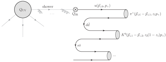
Figure 21: Illustration of the iterative selection of flavours and momenta in the Lund string fragmentation model.

A parton produced in a hard process at some high scale $Q_{\mathrm{UV}}$ emerges from the parton shower, at the hadronization scale $Q_{\mathrm{IR}}$, with 3-momentum $\vec{p}=(\vec{p}_{\perp 0},p_{+})$, where the “+” on the third component denotes “light-cone” momentum, $p_{\pm}=E\pm p_{z}$. Next, an adjacent $d\bar{d}$ pair from the vacuum is created, with relative transverse momenta $\pm p_{\perp 1}$. The fragmenting quark combines with the $\bar{d}$ from the breakup to form a $\pi^{+}$, which carries off a fraction $z_{1}$ of the total lightcone momentum $p_{+}$. The next hadron carries off a fraction $z_{2}$ of the remaining momentum, etc.

For massive endpoints (e.g., $c$ and $b$ quarks, or hypothetical hadronizing new-physics particles, generally called $R$-hadrons), which do not move along straight lightcone sections, the exponential suppression with string area leads to modifications of the form [75], $f(z)\to f(z)/z^{b\,m_{Q}^{2}}$, with $m_{Q}$ the mass of the heavy quark. Strictly speaking, this is the only fragmentation function that is consistent with causality in the string model, though a few alternative forms are typically provided as well.

Note, however, that the term fragmentation function in the context of non-perturbative hadronization models is used to denote only the corrections originating from scales below the infrared cutoff scale of the parton shower. That is, the fragmentation functions introduced here are defined at an intrinsically low scale of order $Q\sim 1\,$GeV. It would therefore be highly inconsistent and misleading to compare them directly to those that are used in fixed-order and/or analytical-resummation contexts, which are typically defined at a factorization scale of order the scale of the hard process.

4.4 Multiple Parton Interactions

In Monte Carlo modeling contexts, multiple parton interactions (MPI) denote the possibility of having multiple partonic $2\to 2$ interactions occurring within a single hadron-hadron collision. The most striking and easily identifiable consequence of MPI is thus arguably the possibility of observing several distinct (i.e., hard) parton-parton interactions in some fraction of hadron-hadron events. Additional jet pairs produced in this way are sometimes referred to as “minijets”, but in the interest of maintaining a compact terminology, we shall here just call them MPI jets. The main distinguishing feature of such jets is that they tend to form back-to-back pairs, with little total $p_{\perp}$. For comparison, jets from bremsstrahlung tend to be aligned with the direction of their “parent” partons. The fraction of multiple interactions that give rise to additional reconstructible jets is, however, quite small (how small depends on the exact jet definition used). Additional soft interactions, below the jet cutoff, are much more plentiful, and can give significant corrections to the colour flow and total scattered energy of the event. This affects the final-state activity in a more global way, increasing multiplicity and summed $E_{T}$ distributions, and contributing to the break-up of the beam remnant in the forward direction.

The first detailed Monte Carlo model for perturbative MPI was proposed by Sjöstrand and van Zijl in [76], and with some variation this still forms the basis for most modern implementations. Here, we therefore focus on that model and on its more recent “interleaved” version [77]. Some discussion of alternative models as well as additional references to the history and development of the subject of multiple interactions can be found in [41].

An intuitive way of arriving at the idea of multiple interactions is to view hadrons simply as ‘bunches’ of incoming partons. No physical law then prevents several distinct pairs of partons from undergoing scattering processes within one and the same hadron-hadron collision. The other key idea to bear in mind is that the exchanged QCD particles are coloured, and hence such multiple interactions — even when soft — can cause non-trivial changes to the colour topology of the colliding system as a whole, with potentially major consequences for the particle multiplicity in the final state.

To begin to construct a model for this, we first observe that, at low $p_{\perp}$, $t$-channel propagators almost go on shell (reminiscent of the case of bremsstrahlung, described in detail in section 2.4), which causes the differential QCD parton-parton scattering cross sections (such as the Rutherford one illustrated in section 2) to become very large, behaving roughly as:

$$\mathrm{d}\hat{\sigma}_{2\to 2}\propto\ \frac{\mathrm{d}\hat{t}}{\hat{t}^{2}}\ \sim\ \frac{\mathrm{d}{{\hat{p}_{\perp}}^{2}}}{{\hat{p}_{\perp}}^{4}}~{},$$ (69)

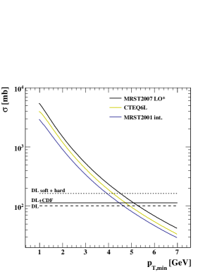
Figure 22: The inclusive jet cross section calculated at LO for three different proton PDFs, compared to various extrapolations of the non-perturbative fits to the total pp cross section at 14 TeV centre-of-mass energy. From [78].

An integration of this cross section from a lower cutoff $p_{\perp\mathrm{min}}$ to $\sqrt{s}$,  using the full (leading-order) QCD $2\to 2$ matrix elements folded with some recent parton-density sets, is shown in figure 22, for $pp$ collisions at 14 TeV [78]. The solid curves, representing the calculated cross sections as functions of $p_{\perp\mathrm{min}}$, are compared to a few different predictions for $\sigma_{\mathrm{tot}}$ (the total $pp$ cross section [79]), shown as horizontal lines with different dashing styles on the same plot. Physically, the jet cross section can of course not exceed the total $pp$ one, yet this is what appears to be happening at scales of order 4–5 GeV in figure 22. How to interpret this behaviour?

Recall that the interaction cross section is an inclusive number. Thus, if a single hadron-hadron event contains two parton-parton interactions, it will count twice in $\sigma_{2\to 2}$ but only once in $\sigma_{\mathrm{tot}}$, and so on for higher parton-parton interaction numbers. In the limit that all the individual parton-parton interactions are independent and equivalent (to be improved on below), we have

$$\sigma_{2\to 2}(p_{\perp\mathrm{min}})=\langle n\rangle(p_{\perp\mathrm{min}})\ \sigma_{\mathrm{tot}}~{},$$ (70)

with $\langle n\rangle(p_{\perp\mathrm{min}})$ giving the average of a Poisson distribution in the number of parton-parton interactions above $p_{\perp\mathrm{min}}$ per hadron-hadron collision,

$$\mathcal{P}_{n}(p_{\perp\mathrm{min}})=\left[\langle n\rangle(p_{\perp\mathrm{min}})\right]^{n}\frac{\exp\left[-\langle n\rangle(p_{\perp\mathrm{min}})\right]}{n!}~{},$$ (71)

and that number may well be above unity. This simple argument in fact expresses unitarity; instead of the total interaction cross section diverging as $p_{\perp\mathrm{min}}\to 0$ (which would violate unitarity), we have restated the problem so that it is now the number of interactions per collision that diverges.

Two important ingredients remain to be introduced in order to fully regulate the remaining divergence. Firstly, the interactions cannot use up more momentum than is available in the parent hadron. This will suppress the large-$n$ tail of the naïve estimate above. Obviously, exact momentum conservation is included in all Monte Carlo models currently on the market, although the details vary somewhat from model to model. In the Pythia-based models [76, 77, 80], the multiple interactions are ordered in $p_{\perp}{}$, and the parton distributions for each successive interaction are explicitly constructed so that the sum of $x$ fractions can never be greater than unity. In the Herwig models [81, 82], instead the uncorrelated estimate of $\langle n\rangle$ above is used directly as an initial guess, but the actual generation of interactions stop once the energy-momentum conservation limit is exceeded (with the last “offending” interaction also removed from consideration).

The second ingredient suppressing the number of interactions, at low $p_{\perp}$ and $x$, is colour screening; if the wavelength $\sim$ $1/p_{\perp}{}$ of an exchanged coloured parton becomes larger than a typical colour-anticolour separation distance, it will only see an average colour charge that vanishes in the limit $p_{\perp}\to 0$, hence leading to suppressed interactions. This screening effectively provides an infrared cutoff for MPI similar to that provided by the hadronization scale for parton showers. A first estimate of an effective lower cutoff due to colour screening would be the proton size

$$p_{\perp\mathrm{min}}\simeq\frac{\hbar}{r_{p}}\approx\frac{0.2~{}\mathrm{GeV}\cdot\mathrm{fm}}{0.7~{}\mathrm{fm}}\approx 0.3~{}\mathrm{GeV}\simeq\Lambda_{\mathrm{QCD}}~{},$$ (72)

but empirically this appears to be too low. In current models, one replaces the proton radius $r_{p}$ in the above formula by a “typical colour screening distance” $d$, i.e. an average size of a region within which the net compensation of a given colour charge occurs. This number is not known from first principles, so effectively this is simply a cutoff parameter, which can then just as well be put in transverse momentum space. The simplest choice is to introduce a step function $\Theta(p_{\perp}{}-p_{\perp\mathrm{min}})$, such that the perturbative cross section completely vanishes below the $p_{\perp\mathrm{min}}$ scale. Alternatively, one may note that the jet cross section is divergent like $\alpha_{s}^{2}(p_{\perp}^{2})/p_{\perp}^{4}$, cf. eq. (69), and that therefore a factor

$$\frac{\alpha_{s}^{2}(p_{\perp 0}^{2}+p_{\perp}^{2})}{\alpha_{s}^{2}(p_{\perp}^{2})}\,\frac{p_{\perp}^{4}}{(p_{\perp 0}^{2}+p_{\perp}^{2})^{2}}$$ (73)

would smoothly regularize the divergences, now with $p_{\perp 0}$ as the free parameter to be tuned to data. Regardless of whether it is imposed as a smooth (Pythia and Sherpa) or steep (Herwig ++) function, this is one of the main “tuning” parameters in such models. Note also that this parameter does not have to be energy-independent. Higher energies imply that parton densities can be probed at smaller $x$ values, where the number of partons rapidly increases. Partons then become closer packed and the colour screening distance $d$ decreases. The uncertainty on the energy and/or $x$ scaling of the cutoff is a major concern when extrapolating between different collider energies.

We now turn to the origin of the so-called “pedestal effect”, the observational fact that hard jets appear to sit on top of a higher “pedestal” of underlying activity than events with no hard jets. This is interpreted as a consequence of impact-parameter-dependence, as follows. In peripheral collisions, only a small fraction of events contain any high-$p_{\perp}$ activity, whereas central collisions are more likely to contain at least one hard scattering; a high-$p_{\perp}$ triggered sample will therefore be biased towards small impact parameters. The ability of a model to describe the shape of the pedestal (e.g., to describe both “minimum-bias” data and underlying-event distributions simultaneously) therefore depends upon its modeling of the impact-parameter dependence, and correspondingly the impact-parameter shape constitutes another main tuning parameter for models that include this dependence.

For each impact parameter, $b$, the number of interactions $\tilde{n}$ can then still be assumed to be distributed according to a Poissonian, eq. (71), again modulo momentum conservation, but now with the mean value of the Poisson distribution depending on impact parameter, $\langle\tilde{n}(b)\rangle$. If the matter distribution has a tail to infinity (as, e.g., Gaussians do), one may nominally obtain events with arbitrarily large $b$ values. In order to obtain finite total cross sections, it is therefore necessary to give a separate interpretation to the “zero bin” of the Poisson distribution, which corresponds to no-interaction events. In models that attempt to describe the entire inelastic non-diffractive cross section, this bin is simply ignored, since the events in it can only represent elastic or diffractive scatterings, which are modeled separately. Alternatively, in models that pertain only to hard inelastic events, it can be reinterpreted as containing that fraction of the total inelastic cross section which do not contain any hard interactions.

Finally, we should mention that there are two perturbative modeling aspects which go beyond the introduction of MPI themselves. In particular, this concerns

1. Parton showers off the MPI.

2. Perturbative parton-rescattering effects.

Without showers, MPI models would generate very sharp peaks for back-to-back MPI jets, caused by unshowered partons passed directly to the hadronization model. However, with the exception of the oldest Pythia 6 model [76], all of the general-purpose event-generator models do include such showers, and hence should exhibit more realistic (i.e., broader and more decorrelated) MPI jets. On the initial state side of the MPI shower issue, the main questions are whether and how correlated multi-parton densities are taken into account, and, as discussed previously, how the showers are regulated at low $p_{\perp}$ and/or low $x$. Although none of the MC models currently impose a rigorous correlated multi-parton evolution, all of them include some elementary aspects. The most significant for parton-level results is arguably momentum conservation, which is enforced explicitly in all the models. The so-called “interleaved” models [74, 77] attempt to go a step further, generating an explicitly correlated multi-parton evolution in which flavour sum rules can be imposed to conserve, e.g., the total numbers of valence and sea quarks across interaction chains.

Perturbative rescattering in the final state occurs if partons are allowed to undergo several distinct interactions, with showering activity possibly taking place inbetween. This has so far not been studied extensively, but a first fairly complete model and exploratory study has been presented in the context of Pythia 8 [80]. In the initial state, parton rescattering effects have so far not been included in any of the general-purpose Monte Carlo models.

4.5 Colour (Re)-Connections and Beam Remnants

Consider now a hadron-hadron collision, i.e., including MPI, at the parton level, equivalent to a resolution scale of about one GeV. The system of coloured partons emerging from the short-distance phase (primary parton-parton interaction plus parton-level underlying event plus beam-remnant partons) must now undergo the transition to colourless hadrons. Infrared sensitive observables, such as individual hadron multiplicities and spectra are crucially dependent on the parton-parton correlations in colour space, and on the properties and parameters of the hadronization model used. Here, we concentrate on the specific issues connected with the structure of the event in colour space.

Keeping the short-distance parts unchanged, the colour structure inside each of the MPI systems is normally still described using just the ordinary leading-colour matrix-element and parton-shower machinery described in sections 2.3 and 2.4. The crucial question, in the context of MPI, is then how colour is neutralized between different MPI systems, including also the remnants. Since these systems can lie at very different rapidities (the extreme case being the two opposite beam remnants), the strings spanned between them can have very large invariant masses (though normally low $p_{\perp}$), and give rise to large amounts of (soft) particle production. Indeed, in the context of soft-inclusive physics, it is precisely these “inter-system” strings which furnish the dominant particle production mechanism, and hence their modeling is an essential part of the infrared physics description.

As discussed more fully in [41], there is a large amount of ambiguity concerning how to address this, and a substantial amount of variation between current models. Experimental investigations of colour reconnections at LEP [83, 84, 85, 86] were only able to exclude some fairly extreme models, with comparatively moderate ones still allowed. Furthermore, in hadron collisions the initial state contains soft colour fields with wavelengths of order the confinement scale. The presence of such fields, unconstrained by LEP measurements, could impact in a non-trivial way the process of colour neutralization [87, 88]. And finally, the MPI produce an additional amount of displaced colour charges, translating to a larger density of hadronizing systems. It is not known to what extent the collective hadronization of such a system differs from a simple sum of independent systems.

A new generation of colour-reconnection toy models have therefore been developed specifically with soft-inclusive and underlying-event physics in mind [89, 90, 91], and also the cluster-based [92] and Generalized-Area-Law [93] models have been revisited in that context. Although still quite crude, these models do appear to be able to describe significant features of the Tevatron and LHC data, such as the $\langle p_{\perp}\rangle(N_{\mathrm{ch}})$ distribution in minimum-bias data, which appears to be quite sensitive to this effect. It is nonetheless clear that the details of the full fragmentation process in hadron-hadron collisions are still far from completely understood.

4.6 Tuning

The main virtue of general-purpose Monte Carlo event generators is their ability to provide a complete and fully differential picture of collider final states, down to the level of individual particles. This allows them to be used as detailed — albeit approximate — theoretical references for measurements performed at accelerators like the LHC, against which models of both known and ‘new’ physics can be tested. As has been emphasized in these lectures, the achievable accuracy depends both on the inclusiveness of the chosen observable and on the sophistication of the simulation itself. An important driver for the latter is obviously the development of improved theoretical models, e.g., by including matching to higher-order matrix elements, more accurate resummations, or better non-perturbative models, as discussed in the previous sections; but it also depends crucially on the available constraints on the remaining free parameters of the model. Using existing data to constrain these is referred to as generator tuning.

Although Monte Carlo models may appear to have a bewildering array of independently adjustable parameters, it is worth keeping at the front of one’s mind that most of these parameters only control relatively small (exclusive) details of the event generation. The majority of the (inclusive) physics is determined by only a few, very important ones, such as, e.g., the value of the strong coupling, in the perturbative domain, and the form of the fragmentation function for massless partons, in the non-perturbative one.

Armed with a good understanding of the underlying model, an expert would therefore normally take a highly factorized approach to constraining the parameters, first constraining the perturbative ones and thereafter the non-perturbative ones, each ordered in a measure of their relative significance to the overall modeling. This factorization, and carefully chosen experimental distributions corresponding to each step, allows one to concentrate on just a few parameters and distributions at a time, reducing the full parameter space to manageable-sized chunks. Still, each step will often involve more than one single parameter, and non-factorizable corrections still imply that changes made in subsequent steps can change the agreement obtained in previous ones by a non-negligible amount, requiring additional iterations from the beginning to properly tune the entire generator framework.

Recent years have seen the emergence of automated tools that attempt to reduce the amount of both computer and manpower required for this task, for instance by making full generator runs only for a limited set of parameter points, and then interpolating between these to obtain approximations to what the true generator result would have been for any intermediate parameter point, as, e.g., in the Professor tool [94, 95]. Automating the human expert input is of course more difficult. In the tools currently on the market, this question is addressed by a combination of input solicited from the generator authors (e.g., which parameters and ranges to consider, which observables constitute a complete set, etc) and the elaborate construction of non-trivial weighting functions that determine how much weight is assigned to each individual bin and to each distribution. The field is still burgeoning, however, and future sophistications are to be expected. Nevertheless, at this point the overall quality of the tunes obtained with automated methods appear to at least be competitive with the manual ones.

A sketch of a reasonably complete tuning procedure, without going into details about the parameters that control each of these sectors in individual Monte Carlo models, would be the following:

1) Keep in mind that inabilities of models to describe data is a vital part of the feedback cycle between theory and experiment. Also keep in mind that perturbation theory at LO$\times$LL is doing very well if it gets within 10% of a given IR safe measurement. An agreement of 5% should be considered the absolute sanity limit, beyond which it does not make any sense whatsoever to tune further. The advent of NLO Monte Carlos may reduce these numbers slightly, but only for quantities for which one expects NLO precision to hold. However, the sanity limit should be taken to be at least twice as large for quantities governed by non-perturbative physics. For some quantities, e.g., ones for which the underlying modeling is known to be poor, an order-of-magnitude agreement or worse may have to be accepted. Attempting to force Monte Carlo models to describe data far outside their domains of validity must be expected to produce similar side effects as attempting to turn a Fiat into a Ferrari merely by cranking up the engine revolutions.

2) Final-State Radiation and Hadronization: mainly using LEP and other $e^{+}e^{-}$ collider data. On the IR safe side, there are event shapes and jet observables, the latter including rates, resolutions, masses, shapes, and jet-jet correlations. On the IR sensitive side, special attention should be paid to the high-$z$ tail of the fragmentation spectra, where a single hadron carries a large fraction of an entire jet’s momentum, since this is the tail that is most likely to give “fake jets”. Depending on the focus of the tuning, attention should also be paid to identified-particle rates and ratios, and to fragmentation in events containing heavy quarks and/or gluon jets. Usually, more weight is given to those particles that are most copiously produced, though this again depends on the focus. Finally, particle-particle correlations and baryon production are typically some of the least well constrained components of the overall modeling. The scaling properties of IR safe vs. IR sensitive contributions can be tested by comparing data at several different $e^{+}e^{-}$ collider energies.

3) Initial-State Radiation, and so-called “Primordial $k_{T}$”: here, one would in principle like to use data from DIS reactions, which are less complicated to interpret than full hadron-hadron collisions. However, due to difficulties in translating between the $ep$ and $pp$ environments, this is normally not what is done in practice. Instead, the main constraining distribution is the dilepton $p_{\perp}$distribution in Drell-Yan events in hadron-hadron collisions. For any observables containing explicit jets, be aware that the underlying event can produce small horizontal shifts in jet $p_{\perp}$ distributions, which may in turn result in seemingly larger-than-expected vertical changes if the distributions are falling sharply. Also note that the ISR evolution is sensitive to the choice of PDFs, with caveats as discussed in section 3.1.

4) Initial-Final Connections: e.g., radiation from colour lines connected to the initial state and jet broadening in hadron collider environments. This is one of the most poorly controlled parts of most MC models. Keep in mind that it is not directly constrained by pure final-state observables, such as LEP fragmentation, nor by pure initial-state observables, such as the Drell-Yan $p_{\perp}$ spectrum, which is why we list it as a separate item here. In principle, DIS would again be a prime territory for placing constraints on this aspect at least for quark jets, but in practice more often inclusive-jet and other multi-jet processes (such as $W/Z+\,$jets) in hadron colliders are used.

5) Underlying Event: Good constraints on the overall level of the underlying event can be obtained by counting the summed transverse energy (more IR safe) and/or particle multiplicities and average transverse momenta (more IR sensitive) in regions transverse to a hard trigger jet (more IR safe) or particle (more IR sensitive). Constraints on the fluctuations of the underlying event are also important, and can be obtained, e.g., by comparing to measurements of the RMS of such distributions. Again, note that the UE is sensitive to the choice of PDFs.

6) Colour (Re-)Connections and other Final-State Interactions: By Final-State Interactions, we intend a broad spectrum of possible collective effects that may be included to a greater or lesser extent in various models. These effects include: Bose-Einstein correlations, colour reconnections, hydrodynamics, string interactions, Cronin effect, etc. As a rule, these effects are non-perturbative and hence should not modify IR safe observables appreciably. They can, however, have drastic effects on IR sensitive ones, such as particle multiplicities, and particle momentum distributions, wherefore useful constraints are typically furnished by particle-particle correlations, by measurements of particle momentum spectra as functions of quantities believed to serve as indicators of the strength of these phenomena (such as event multiplicity), and/or by collective-flow-type measurements. Finally, if the model includes a universal description of underlying event and soft-inclusive QCD, as many MPI-based models do, then minimum-bias data can also be used as a control sample, though one must then be careful either to address diffractive contributions properly or to include only data samples that minimize their impact.

7) Beam Remnants: Constraints on beam remnant fragmentation are most easily obtained in the forward region, but, e.g., the amount of baryon transport from the remnant to a given rapidity region can also be used to probe how much the colour structure of the remnant was effectively disturbed, with more baryon transport indicating a larger amount of “beam baryon blowup”.

We round off by emphasizing that comparisons of specific models and tunes to data can be useful both as immediate tests of commonly used models, and to illustrate the current amount of theoretical uncertainty surrounding a particular distribution. Independently of how well the models fit the data, such comparisons also provide a set of well-defined theoretical reference curves that serve as useful guidelines for future studies. However, the conclusions that can be drawn from comparisons of individual tunes of specific models on single distributions are necessarily limited. In order to obtain more general conclusions, a strategy for a more coherent and over-arching look at both the data and the models was recently proposed in [96]. Specifically, rather than performing one global tune to all the data, as is usually done, a more systematic check on the validity of the underlying physics model can be obtained by instead performing several independent optimizations of the model parameters for a range of different phase space windows and/or collider environments. In regions in which consistent parameter sets are obtained, with predictions that are acceptably close to the data, the underlying model can then be considered as interpolating well, i.e., it is universal. If not, a breakdown in the ability of the model ability to span different physical regimes has been identified, and can be addressed, with the nature of the deviations giving clues as to the nature of the breakdown. With the advent of automated tools making it easier to run several optimizations without much additional computing overhead, such systematic studies are now becoming feasible, with a first example given in [96].

References

- [1] K. A. Brueckner, Phys.Rev. 86, 106 (1952).
- [2] O. Greenberg, Phys.Rev.Lett. 13, 598 (1964).
- [3] M. Han and Y. Nambu, Phys.Rev. 139, B1006 (1965).
- [4] R. Ellis, W. Stirling, and B. Webber, QCD and collider physics (Camb. Monogr. Part. Phys. Nucl. Phys. Cosmol., 1996).
- [5] M. E. Peskin and D. V. Schroeder, (1995).
- [6] T. Plehn, D. Rainwater, and P. Z. Skands, Phys.Lett. B645, 217 (2007), hep-ph/0510144.
- [7] P. Z. Skands, T. Plehn, and D. Rainwater, (2005), hep-ph/0511306.
- [8] J. Alwall, S. de Visscher, and F. Maltoni, JHEP 0902, 017 (2009), 0810.5350.
- [9] A. Papaefstathiou and B. Webber, JHEP 06, 069 (2009), 0903.2013.
- [10] D. Krohn, L. Randall, and L.-T. Wang, (2011), 1101.0810.
- [11] C. K. Vermilion, (2011), 1101.1335.
- [12] S. Bethke, Eur.Phys.J. C64, 689 (2009), 0908.1135.
- [13] G. Dissertori et al., JHEP 0908, 036 (2009), 0906.3436.
- [14] A. Pukhov, (2004), hep-ph/0412191.
- [15] CompHEP Collaboration, E. Boos et al., Nucl.Instrum.Meth. A534, 250 (2004), hep-ph/0403113.
- [16] J. Alwall et al., JHEP 0709, 028 (2007), 0706.2334.
- [17] A. Kanaki and C. G. Papadopoulos, Comput.Phys.Commun. 132, 306 (2000), hep-ph/0002082.
- [18] F. Krauss, R. Kuhn, and G. Soff, JHEP 0202, 044 (2002), hep-ph/0109036.
- [19] M. Moretti, T. Ohl, and J. Reuter, (2001), hep-ph/0102195.
- [20] M. Bähr et al., Eur.Phys.J. C58, 639 (2008), 0803.0883.
- [21] T. Gleisberg and S. Hoeche, JHEP 0812, 039 (2008), 0808.3674.
- [22] G. Dissertori, I. Knowles, and M. Schmelling, (2003).
- [23] CTEQ Collaboration, R. Brock et al., Rev.Mod.Phys. 67, 157 (1995).
- [24] Y. I. Azimov, Y. L. Dokshitzer, V. A. Khoze, and S. I. Troyan, Z. Phys. C27, 65 (1985).
- [25] G. P. Salam, (2010), 1011.5131.
- [26] A. Banfi, G. P. Salam, and G. Zanderighi, JHEP 1006, 038 (2010), 1001.4082.
- [27] CMS Collaboration, V. Khachatryan et al., (2011), 1102.0068.
- [28] K. Wraight and P. Skands, (2011), 1101.5215.
- [29] F. James, Rept. Prog. Phys. 43, 1145 (1980).
- [30] R. Kleiss, W. Stirling, and S. Ellis, Comput.Phys.Commun. 40, 359 (1986).
- [31] G. Lepage, J.Comput.Phys. 27, 192 (1978), Revised version.
- [32] G. P. Lepage, (1980), CLNS-80/447.
- [33] P. D. Draggiotis, A. van Hameren, and R. Kleiss, Phys.Lett. B483, 124 (2000), hep-ph/0004047.
- [34] W. Giele, D. Kosower, and P. Skands, (2011), 1102.2126.
- [35] J. Lopez-Villarejo and P. Skands, JHEP 1111, 150 (2011), 1109.3608.
- [36] T. Kinoshita, J. Math. Phys. 3, 650 (1962).
- [37] T. D. Lee and M. Nauenberg, Phys. Rev. 133, B1549 (1964).
- [38] P. Richardson, JHEP 11, 029 (2001), hep-ph/0110108.
- [39] S. Catani, B. R. Webber, and G. Marchesini, Nucl. Phys. B349, 635 (1991).
- [40] M. A. Gigg and P. Richardson, (2008), 0805.3037.
- [41] A. Buckley et al., (2011), 1101.2599, Accepted for publication in Physics Reports.
- [42] T. Sjöstrand, (2006), hep-ph/0611247.
- [43] Particle Data Group, K. Nakamura, J. Phys. G37, 075021 (2010).
- [44] NLO Multileg Working Group, Z. Bern et al., p. 83 (2008), 0803.0494.
- [45] T. Sjöstrand, (2009), 0911.5286.
- [46] G. Gustafson and U. Pettersson, Nucl. Phys. B306, 746 (1988).
- [47] S. Catani and M. H. Seymour, Nucl. Phys. B485, 291 (1997), hep-ph/9605323.
- [48] A. Gehrmann-De Ridder, T. Gehrmann, and E. W. N. Glover, JHEP 09, 056 (2005), hep-ph/0505111.
- [49] S. Schumann and F. Krauss, JHEP 03, 038 (2008), 0709.1027.
- [50] G. Corcella et al., JHEP 01, 010 (2001), hep-ph/0011363.
- [51] M. H. Seymour, Nucl. Phys. B436, 443 (1995), hep-ph/9410244.
- [52] M. H. Seymour, Comp. Phys. Commun. 90, 95 (1995), hep-ph/9410414.
- [53] S. Catani, F. Krauss, R. Kuhn, and B. R. Webber, JHEP 11, 063 (2001), hep-ph/0109231.
- [54] L. Lönnblad, JHEP 05, 046 (2002), hep-ph/0112284.
- [55] S. Mrenna and P. Richardson, JHEP 05, 040 (2004), hep-ph/0312274.
- [56] N. Lavesson and L. Lönnblad, JHEP 07, 054 (2005), hep-ph/0503293.
- [57] M. L. Mangano, M. Moretti, F. Piccinini, and M. Treccani, JHEP 01, 013 (2007), hep-ph/0611129.
- [58] N. Lavesson and L. Lönnblad, JHEP 12, 070 (2008), 0811.2912.
- [59] S. Frixione and B. R. Webber, JHEP 06, 029 (2002), hep-ph/0204244.
- [60] S. Frixione, P. Nason, and B. R. Webber, JHEP 08, 007 (2003), hep-ph/0305252.
- [61] S. Frixione and B. R. Webber, (2008), 0812.0770.
- [62] S. Frixione, P. Nason, and C. Oleari, JHEP 11, 070 (2007), 0709.2092.
- [63] K. Hamilton and P. Nason, JHEP 06, 039 (2010), 1004.1764.
- [64] M. Bengtsson and T. Sjöstrand, Nucl. Phys. B289, 810 (1987).
- [65] M. Bengtsson and T. Sjöstrand, Phys. Lett. B185, 435 (1987).
- [66] T. Sjöstrand, S. Mrenna, and P. Skands, JHEP 05, 026 (2006), hep-ph/0603175.
- [67] T. Sjöstrand, S. Mrenna, and P. Skands, Comput. Phys. Commun. 178, 852 (2008), 0710.3820.
- [68] X. Artru and G. Mennessier, Nucl. Phys. B70, 93 (1974).
- [69] B. Andersson, The Lund model (Camb. Monogr. Part. Phys. Nucl. Phys. Cosmol., 1997).
- [70] B. Andersson, G. Gustafson, and T. Sjöstrand, Nucl. Phys. B197, 45 (1982).
- [71] B. Andersson, G. Gustafson, and T. Sjostrand, Phys.Scripta 32, 574 (1985).
- [72] P. Eden and G. Gustafson, Z.Phys. C75, 41 (1997), hep-ph/9606454.
- [73] T. Sjöstrand and P. Z. Skands, Nucl. Phys. B659, 243 (2003), hep-ph/0212264.
- [74] T. Sjöstrand and P. Z. Skands, JHEP 03, 053 (2004), hep-ph/0402078.
- [75] M. G. Bowler, Z. Phys. C11, 169 (1981).
- [76] T. Sjöstrand and M. van Zijl, Phys. Rev. D36, 2019 (1987).
- [77] T. Sjöstrand and P. Z. Skands, Eur. Phys. J. C39, 129 (2005), hep-ph/0408302.
- [78] M. Bähr, J. M. Butterworth, and M. H. Seymour, JHEP 01, 065 (2009), 0806.2949.
- [79] A. Donnachie and P. V. Landshoff, Phys. Lett. B296, 227 (1992), hep-ph/9209205.
- [80] R. Corke and T. Sjöstrand, JHEP 01, 035 (2009), 0911.1909.
- [81] J. M. Butterworth, J. R. Forshaw, and M. H. Seymour, Z. Phys. C72, 637 (1996), hep-ph/9601371.
- [82] M. Bähr, J. M. Butterworth, S. Gieseke, and M. H. Seymour, (2009), 0905.4671.
- [83] OPAL, G. Abbiendi et al., Phys. Lett. B453, 153 (1999), hep-ex/9901019.
- [84] OPAL, G. Abbiendi et al., Eur. Phys. J. C45, 291 (2006), hep-ex/0508062.
- [85] ALEPH, S. Schael et al., Eur. Phys. J. C48, 685 (2006), hep-ex/0604042.
- [86] DELPHI, J. Abdallah et al., Phys. Lett. B643, 147 (2006), hep-ex/0610031.
- [87] W. Buchmuller and A. Hebecker, Phys. Lett. B355, 573 (1995), hep-ph/9504374.
- [88] A. Edin, G. Ingelman, and J. Rathsman, Phys. Lett. B366, 371 (1996), hep-ph/9508386.
- [89] M. Sandhoff and P. Z. Skands, FERMILAB-CONF-05-518-T, in hep-ph/0604120.
- [90] P. Z. Skands and D. Wicke, Eur.Phys.J. C52, 133 (2007), hep-ph/0703081.
- [91] P. Z. Skands, Phys.Rev. D82, 074018 (2010), 1005.3457.
- [92] B. R. Webber, J. Phys. G24, 287 (1998), hep-ph/9708463.
- [93] J. Rathsman, Phys. Lett. B452, 364 (1999), hep-ph/9812423.
- [94] A. Buckley, H. Hoeth, H. Lacker, H. Schulz, and E. von Seggern, p. 267 (2009), 0906.0075.
- [95] A. Buckley, H. Hoeth, H. Lacker, H. Schulz, and J. E. von Seggern, Eur. Phys. J. C65, 331 (2010), 0907.2973.
- [96] H. Schulz and P. Skands, (2011), 1103.3649.
- [97] N. Ellis et al., (2009), CERN-2009-002.
- [98] C. Grojean et al., (2010), 1012.4643.
- [99] N. Ellis et al., (2008), CERN-2008-007.