Using Channel Output Feedback to Increase Throughput in Hybrid-ARQ

Abstract

Hybrid-ARQ protocols have become common in many packet transmission systems due to their incorporation in various standards. Hybrid-ARQ combines the normal automatic repeat request (ARQ) method with error correction codes to increase reliability and throughput. In this paper, we look at improving upon this performance using feedback information from the destination, in particular, using a powerful forward error correction (FEC) code in conjunction with a proposed linear feedback code for the Rayleigh block fading channels. The new hybrid-ARQ scheme is initially developed for full received packet feedback in a point-to-point link. It is then extended to various different multiple-antenna scenarios (MISO/MIMO) with varying amounts of packet feedback information. Simulations illustrate gains in throughput.

I Introduction

The tremendous growth in demand for throughput in wireless networks warrants new design principles for coding information at the lower layers. In recent years, packet-based hybrid automatic repeat request (ARQ), which integrates forward error correction (FEC) coding with the traditional automatic repeat request protocol, has sparked much interest. Any hybrid-ARQ scheme includes the transmission of an acknowledgement (ACK) or a negative-acknowledgement (NACK) from the destination to the source. Although not normally viewed this way, the feedback of ACK/NACK can be seen as a form of channel output information (COI) indicating to the source the ‘quality’ of the channel output. Exploiting the full potential of COI at the source for hybrid-ARQ schemes, however, has not been explored in the literature. In fact most of the discussion about feedback in wireless systems has been limited to the use of channel state information (CSI) at the source [1, 2, 3].

Research since the 1960s [4, 5, 6] has long established the utility of using COI at the source to increase reliability in additive white Gaussian noise (AWGN) channels. The gain in reliability scales very fast in blocklength and relies on simple, linear coding schemes. These schemes achieve a doubly exponential decay in the probability of error as a function of the number of packet retransmissions; this is in stark contrast to open loop systems (without COI) that can achieve only singly exponential decay in the probability of error. Most of the the literature for COI assumes an information-theoretic perspective for analysis. In this work, however, we take a more signal processing approach to COI. In particular, we explore the efficacy of including COI to increase the throughput of a practical hybrid-ARQ scheme.

As is commonly done in hybrid-ARQ literature, we assume that the transmissions will take place over a block fading channel where the fading characteristics of the channel are assumed to be constant over the transmission of a packet (e.g., [7, 8, 9, 10]). In the context of this channel, there will be two main types of side-information that we consider to be available at the source: CSI and COI. CSI is commonly known as a complex-valued quantity that represents the spatial alignment of the channel. This can be either outdated, where the source has access to outdated values of CSI (i.e., the channel states for previous blocks), or current, where the source has access to the present value of CSI (i.e., the channel state for the current block). Outdated CSI is commonly obtained through feedback techniques from the destination. Current CSI can be obtained through numerous methods such as exploiting channel reciprocity through time division duplexing. In fact, most recent standards [11] and technologies like multi-user MIMO, network MIMO, and OFDM incur major penalties in performance without the availability of current CSI [12, 13, 14]. The most common form of COI is simply the past received packet at the destination; we will be using this definition as the destination incurs no processing before feeding back the received packet. The main focus of the paper will be the integration of COI in to a hybrid-ARQ framework.

Hybrid-ARQ improves the reliability of the transmission link by jointly encoding or decoding the information symbols across multiple received packets. Specifically, there are three ways [15] in which hybrid-ARQ schemes are implemented:

• Type I: Packets are encoded using a fixed-rate FEC code, and both information and parity symbols are sent to the destination. In the event that the destination is not able to decode the packet, it rejects (NACK) the current transmission and requests the retransmission of the same packet from the source. Subsequent retransmissions from the source are merely a repetition of the first transmission.

• Type II: In this case, the destination has a buffer to store previous unsuccessfully transmitted packets. The first packet sent consists of the FEC code and each subsequent retransmission consists of only the parity bits (incremental redundancy) to help the receiver at the destination jointly decode across many retransmissions of the same packet.

• Type III: This method is similar to Type II with one major difference. In Type III, every retransmission is self decodable, e.g., Chase combining[16]. Therefore the destination has the flexibility to either combine the current retransmission with all the previously received retransmissions or use only the current packet for decoding.

The first mention of hybrid-ARQ techniques can be traced back to papers from the 1960s (e.g., [17]). However, most attention to this protocol has been given during the late 1990s and early 2000s. Throughput and delay analyses were done for the Gaussian collision channel in [7, 18, 8, 9]. These topics were also investigated for wireless multicast in [10] and for block fading channels with modulation constraints in [19]. The hybrid-ARQ technique has been looked at when using many different types of FEC codes including turbo codes [20, 21, 22], convolutional codes [8, 23], LDPC codes [9, 24], and Raptor codes [25, 26]. The performance analysis of a hybrid-ARQ scheme with CSI[2, 3, 27, 28, 29] and without CSI at the source[30] has also been studied in the literature. In addition, different ways to utilize the feedback channel have been investigated in [31, 32].

In this work, however, we explore the advantages of combining conventional CSI feedback with COI feedback. As we noted earlier, the potential of COI feedback in hybrid-ARQ has not been properly explored. The method we introduce is a variation of Type III hybrid-ARQ scheme that incorporates the use of COI feedback. In the event that no COI feedback is available, our proposed scheme simply reduces to the regular Chase combining in which packets are repeated for retransmission and the destination combines the received packets using maximum ratio combining (MRC). However when COI feedback is available, we look at implementing a linear feedback code that is a generalization of Chase combining to increase the performance of the packet transmission system. A linear feedback code is simply a transmission scheme in which the transmit value is a strictly linear function of the message to be sent and the feedback side-information [33]. We show that such codes provide advantages over merely repeating the last packet, while offering simpler analysis and implementation than conventional Type II incremental redundancy codes.

A relevant concern for the implementation of COI feedback techniques is practicality as it requires (possibly) sending large amounts of data from the destination back to the source. However, we hope to address these concerns by first studying the ideal scenarios (i.e., perfect COI feedback by feeding back the full received packet) to illustrate what is theoretically possible and then extend these results to limited-resource cases (i.e., noisy COI feedback and feeding back only parts of the received packet). This allows us to establish a trade-off in performance to allow for practical limitations on the system. Furthermore, COI feedback techniques can be especially beneficial when there is link asymmetry between the source and the destination. In other words, the situations in which the reverse link can support much higher rates than the forward link.

To accommodate the use of multiple-input single-output (MISO) and multiple-input multiple-output (MIMO) systems, we first construct the proposed scheme for the simplest case of single-input single-output (SISO) transmission and then extend the scheme to the case with multiple transmit antennas. Specifically, the scheme is adapted for use with MISO and MIMO when current CSI is available at the source and either perfect or noisy COI feedback is available. It is also adapted for MIMO when perfect COI and only outdated CSI is available at the source.

The paper is structured as follows. In Section II, a brief high-level description of hybrid-ARQ is given to motivate the investigation into using more feedback in a packet retransmission scheme. In Section III, the feedback scheme to be integrated into a hybrid-ARQ protocol is introduced for SISO systems. We begin the section by describing the encoding process. It is followed by a discussion of decoding; this involves two different cases - systems with noiseless COI feedback and systems with noisy COI feedback. In Section IV, the SISO scheme is extended to various multiple antenna scenarios. In Section V, the overall hybrid-ARQ system is discussed in detail where now the COI feedback schemes created are integrated as a generalization of Chase combining. Schemes that vary the amount of COI feedback being sent to the source are also discussed. In Section VI, throughput simulations are given to illustrate the performance of the proposed hybrid-ARQ scheme versus other commonly used hybrid-ARQ schemes such as [34] and traditional Chase combining. Note that our comparison is with the incremental redundancy ARQ scheme in [34] (not the standardized system in general). It is not our intention to assume the same conditions present in the transport channels as the ones discussed in [34].

Notation:

The vectors (matrices) are represented by lower (upper) boldface letters while scalars are represented by lower italicized letters. The operators $(\cdot)^{T},(\cdot)^{*},\textrm{tr}(\cdot)$, and $\lVert\cdot\rVert$ denote the transpose, conjugate transpose, trace, and Euclidean norm of a matrix/vector respectively. The expectation of a random variable or matrix/vector is denoted by $E[\cdot]$. The boldface letter ${\mathbf{I}}$ represents the identity matrix.

II System Model

Consider using the SISO hybrid-ARQ transmission system in Fig. 1 where there is one antenna available at the source and the destination. The goal of the transmission scheme is to successfully send the binary information packet, ${\mathbf{m}}\in GF(2)^{L_{\rm{info}}}$, to the destination over a maximum of $N$ packet retransmissions. $GF(2)$ denotes the Galois field with just two elements $\{0,1\}$, and $L_{\rm{info}}$ denotes the total number of information bits. Transmission is accomplished by first encoding the information packet using a rate $L_{\rm{info}}/L_{\rm{coded}}~{}(\textrm{where }L_{\rm{info}}\leq L_{\rm{coded}})$ FEC code, producing a binary codeword of length $L_{\rm{coded}}$ referred to as ${\mathbf{c}}\in GF(2)^{L_{\rm{coded}}}$. The codeword is then modulated using a source constellation $\Theta[N]$ (e.g., QAM, QPSK, etc.) to create a length $L$ packet of modulation symbols called ${\boldsymbol{\theta}}\in\mathbb{C}^{1\times L}$. Note that the source constellation $\Theta[N]$ is a function of the maximum number of transmissions $N$. If $N$ is large for a fixed $L$ (i.e., $L/N$ is small), we may decide to choose a denser constellation to achieve higher throughput. This is then processed by a packet encoder that encapsulates most of the hybrid-ARQ process. At this stage, the modulated symbols are further encoded to generate the transmitted signal ${\mathbf{x}}[k]\in\mathbb{C}^{1\times L}$. It is worthwhile to contrast that ${\boldsymbol{\theta}}$ is the packet of desired information symbols and the entries of ${\mathbf{x}}[k]$ are the actual signals sent at each channel use to convey that information to the destination. Note that some quantities have a retransmission index, $k$, which refers to time on the packet level (i.e., for each $k$ a length $L$ signal, ${\mathbf{x}}[k]$, is transmitted). Furthermore, the transmit vector is constrained by the power constraint at the source given by

$$E\left[|{\mathbf{x}}[k]|^{2}\right]\leq L\rho,\quad k=1,\ldots,N,$$ (1)

where, as mentioned, $N$ is the maximum number of retransmissions allowed and $\rho>0$ is the average power per channel use.

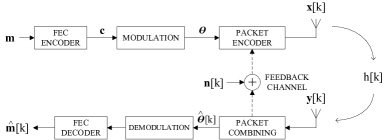
Figure 1: The hybrid-ARQ transmission system

At the destination, the $k^{th}$ retransmission received signal, ${\mathbf{y}}[k]\in\mathbb{C}^{1\times L}$, is obtained. Using this setup, ${\mathbf{y}}[k]$ can be written as

$${\mathbf{y}}[k]=h[k]{\mathbf{x}}[k]+{\mathbf{z}}[k],\quad 1\leq k\leq N,$$ (2)

where ${\mathbf{z}}[k]\in\mathbb{C}^{1\times L}$ is additive noise whose entries are i.i.d. complex Gaussian such that ${\mathbf{z}}[k]\sim{\mathcal{C}}{\mathcal{N}}(0,{\mathbf{I}})$, and $h[k]\in\mathbb{C}$ is a zero-mean complex Gaussian random variable with unit variance. Therefore, we assume that the retransmission takes place across a Rayleigh block fading channel with blocklength $L$. Note that ${\mathbf{x}},{\mathbf{y}},$ and ${\mathbf{z}}$ have been defined as row vectors; this is to aid the later extension of the scheme to a MISO/MIMO setting. After retransmission $k$, the received packet is combined using all previously received packets to create an estimate of the original modulated information packet, $\widehat{{\boldsymbol{\theta}}}[k]$. The combining stage, in Chase combining for example, combines all the received realizations for a given symbol using MRC. Improving upon the encoding and combining steps using COI forms the main thrust of this paper; this will be discussed in detail in the next section. It is worth pointing out that the incorporation of COI feedback into the hybrid-ARQ scheme is being implemented at the physical layer. After combining at the destination, the packet is then demodulated using either soft or hard decoding methods and then passed to the FEC decoder which then outputs a final estimate of the original information packet, $\widehat{{\mathbf{m}}}[k]$.

It is important to note that a feedback channel is present between the destination and the source. In fact, for any ARQ protocol, a feedback channel is necessary so the destination can send back an ACK/NACK signal. In our setup, we assume that:

• The destination does not only send back ACK/NACK information but also feeds back CSI which could be outdated, current, or quantized.

• The destination can feed back the COI for the packet to the source where COI feedback is simply the destination feeding back exactly (or a subset of) what it has received. This is discussed further in Section V.

Explicitly, the causal COI at the source is equivalent to the source having access to the past values of ${\mathbf{y}}[k]$. However, since noisy COI feedback is also investigated, we introduce a feedback noise process ${\mathbf{n}}[k]$ (see Fig. 1) so that the source now only has access to past values of ${\mathbf{y}}[k]+{\mathbf{n}}[k]$. Note that the source might have access to all or only some of the entries in ${\mathbf{y}}[k]+{\mathbf{n}}[k]$ based on how much COI is being fed back. Furthermore, the source can subtract out what it sent due to the availability of $h[k]$. Therefore, this is analogous to having access to past values of ${\mathbf{z}}[k]+{\mathbf{n}}[k]$. The feedback noise, ${\mathbf{n}}[k]$, is assumed to be complex AWGN such that ${\mathbf{n}}[k]\sim{\mathcal{C}}{\mathcal{N}}(0,\sigma^{2}{\mathbf{I}})$ and also independent of the forward noise process, ${\mathbf{z}}[k]$. Note that setting $\sigma^{2}=0$ yields perfect COI feedback as a special case.

III Linear Feedback Combining

We now narrow our focus to the packet encoding/combining steps of the hybrid-ARQ system; the full system including the FEC will be considered in Section V. Specifically, we consider employing COI feedback to better refine the destination’s packet estimate $\widehat{{\boldsymbol{\theta}}}[k]$ after each retransmission. Improving the quality of the estimate will lead to fewer decoding errors and higher throughput. To begin, we look at the most straightforward setup of SISO, where the source and destination each have one antenna and outdated CSI along with causal COI, whether it be noisy or perfect. The scheme will be extended for use with multiple antenna scenarios and the effects of varying the CSI feedback will be discussed in Section IV.

III-A Overview

To construct the new transmission strategy, we aim to develop a linear coding scheme with the objective of maximizing the post-processed signal-to-noise ratio (SNR) after $N$ retransmissions. Initially, we focus on sending only one symbol or, in other words, assume that $L=1$ where the information packet ${\boldsymbol{\theta}}$ is now a scalar, $\theta\in\mathbb{C}$. Note that this assumption is only done to reduce the amount of notation—the proposed scheme can be readily extended to arbitrary packet lengths as it is assumed that it will be utilized, in general, for $L\gg 1$. In the case that $L=1$, however, the transmit and received vectors ${\mathbf{x}}[k]$ and ${\mathbf{y}}[k]$ also reduce to scalars $x[k]$ and $y[k]$.

It is helpful at this stage to introduce a mathematical framework for linear feedback coding. It can be seen that if $L=1$, then, gathering all packet transmissions together, (2) can be rewritten as

$${\mathbf{y}}={\mathbf{D}}{\mathbf{x}}+{\mathbf{z}},$$ (3)

where ${\mathbf{y}}=\left[y[1],y[2],\ldots,y[N]\right]^{T}$ is a column vector (likewise for ${\mathbf{x}}$ and ${\mathbf{z}}$) and ${\mathbf{D}}=\mathrm{diag}(h[1],h[2],\ldots,h[N])$ is a matrix formed with the channel coefficients down the diagonal. Note that the notation ${\mathbf{D}}$ is chosen to give distinction between it and the commonly-used ${\mathbf{H}}$ for a MIMO channel matrix which is used later in the paper. With this setup, we can write the transmit vector ${\mathbf{x}}$ as

$${\mathbf{x}}={\mathbf{g}}\theta+{\mathbf{F}}({\mathbf{z}}+{\mathbf{n}}),$$ (4)

where ${\mathbf{g}}\in\mathbb{C}^{N\times 1}$ is the vector used to encode the symbol to be sent, $\theta$, and ${\mathbf{F}}\in\mathbb{C}^{N\times N}$ is a strictly lower triangular matrix used to encode the side-information $\{{\mathbf{z}}+{\mathbf{n}}\}$. The form of ${\mathbf{F}}$ is constrained to be strictly lower triangular to enforce causality. Note that (4) is the transmit structure of linear feedback coding—the transmitted value is a linear function of the side-information and of the information message. Furthermore, the encoding process is encapsulated by the matrix ${\mathbf{F}}$ and the vector ${\mathbf{g}}$.

Now, we shift focus to the destination. After receiving a packet, the destination forms an estimate of the packet by

$$\widehat{\theta}[k]={\mathbf{q}}_{k}^{*}{\mathbf{y}}_{(k)},$$ (5)

where $\widehat{\theta}[k]$ is the destination’s estimate of the symbol $\theta$ after $k$ retransmissions, ${\mathbf{q}}_{k}\in\mathbb{C}^{N\times 1}$ is the combining vector used for the $k^{th}$ retransmission, and the notation ${\mathbf{y}}_{(k)}$ refers to the first $k$ entries of ${\mathbf{y}}$. It can be seen that the packet estimation process can be completely described by the vectors ${\mathbf{q}}_{k}$. Thus, the entire linear feedback code can be represented by the tuple $({\mathbf{g}},{\mathbf{F}},{\mathbf{q}}_{k})$ [33]. Thus, with this framework, the post-processed SNR for the system after $N$ retransmissions can be defined as

$$SNR=\frac{|{\mathbf{q}}^{*}{\mathbf{D}}{\mathbf{g}}|^{2}\rho}{\|{\mathbf{q}}^{*}({\mathbf{I}}+{\mathbf{D}}{\mathbf{F}})\|^{2}+\sigma^{2}\|{\mathbf{q}}^{*}{\mathbf{D}}{\mathbf{F}}\|^{2}}.$$ (6)

where ${\mathbf{q}}={\mathbf{q}}_{N}$; the subscript is dropped for convenience. We can now mathematically define the overall objective of this section: to construct a linear feedback code that maximizes the post-processed SNR given the channel coefficients $h[k]$; this is equivalent to finding

$$({\mathbf{g}},{\mathbf{F}},{\mathbf{q}})_{opt}=\mathop{\mathrm{argmax}}_{({\mathbf{g}},{\mathbf{F}},{\mathbf{q}})}\frac{|{\mathbf{q}}^{*}{\mathbf{D}}{\mathbf{g}}|^{2}\rho}{\|{\mathbf{q}}^{*}({\mathbf{I}}+{\mathbf{D}}{\mathbf{F}})\|^{2}+\sigma^{2}\|{\mathbf{q}}^{*}{\mathbf{D}}{\mathbf{F}}\|^{2}},$$ (7)

while satisfying the average power constraint (1) and causality of side-information.

In the special case of a SISO system with perfect COI ($\sigma^{2}=0$) and causal CSI, it can be shown that the solution to (7) has the structure of the scheme given in [35] (the specific derivation is omitted due to space concerns). Interestingly, the scheme in that work was derived using a control-theoretic approach instead of using post-processed SNR as an objective function [36]. Most importantly, the optimality of the scheme in the SNR sense motivates our construction. In particular, we develop a generalization of the feedback scheme presented in [35] as this scheme was not only shown to achieve capacity but also achieve a doubly exponential decay in probability of error. In the proposed generalized scheme, we extend the original scheme for use with:

• single and multiple antennas (i.e., MISO and MIMO wireless systems),

• perfect and noisy COI feedback,

• outdated and current CSI at the source.

The details of the proposed scheme are given in the following sections.

III-B Encoding

The fundamental idea of the transmission scheme is to transmit the scaled estimation error from the previous transmission for each successive retransmission so that the destination can attempt to correct its current estimate [37, 38]. The scaling operation is performed so the transmitted signal meets the average power constraint (1). To further illustrate this concept and help motivate our construction, we now briefly present a heuristic overview of the scheme in [35]. In this case, the transmitted signal, $x[k]$, is given as

$$x[k+1]=\delta[k]e[k],$$ (8)

where $e[k]=\theta-\widehat{\theta}[k]$ is the error in the destination’s estimate of the message after the $k^{th}$ packet reception and $\delta[k]$ is the scaling factor chosen to appease the power constraint. After receiving $y[k]$, the destination then forms an estimate of the error, $\widehat{e}[k]$. This is then subtracted from the current estimate. As will be shown, our proposed scheme is motivated by this error-scaling technique.

We now define how the source encodes the message. As the encoding process for a perfect COI feedback and the encoding process for a noisy COI feedback are very similar, we now introduce the encoding process for both perfect and noisy COI feedback in a single framework. The encoding operation of the proposed scheme can be written compactly in the definitions of ${\mathbf{F}}$ and ${\mathbf{g}}$; they are constructed as:

• The $(i,j)^{th}$ entry of ${\mathbf{F}}$, $f_{i,j}$, is

  $$f_{i,j}=\left\{\begin{array}[]{l r}-\sqrt{\gamma}\rho\phi[i-1]h^{*}[j],&i>j,\\ 0,&i\leq j,\end{array}\right.$$

• The $i^{th}$ entry of ${\mathbf{g}}$, $g_{i}$, is

  $$g_{i}=\phi[i-1],$$

where

$$\phi[k]=\left\{\begin{array}[]{l r}\displaystyle\prod_{i=1}^{k}\beta_{(\gamma,\sigma^{2})}[i],&k>0\\ 1,&k=0,\\ \end{array}\right.$$

$$\beta_{(\gamma,\sigma^{2})}[k]=\left(1+(1+\sigma^{2})\gamma\rho|h[k]|^{2}\right)^{-1/2},$$ (9)

and $\gamma\in[0,1]$ is a constant. Note that the scaling factor $\delta[k]$ in (8) is now given its analog by the term $\phi[k]$ which ensures the proposed scheme meets the power constraint (1).

The scheme presented here in the form of ${\mathbf{g}}$ and ${\mathbf{F}}$ is a direct generalization of the error-scaling scheme in (8) as the original scheme for perfect COI feedback can be obtained as a special case of these definitions by letting $\gamma=1$ and $\sigma^{2}=0$. The main mechanism introduced into the proposed scheme is a power allocation variable, $\gamma$, to help combat the effect of the feedback noise, $n[k]$ [33]. Specifically, $\gamma$ is a degree of freedom introduced to allocate power between the encoding of feedback side-information and the information to be sent. It is only of use when the feedback channel is noisy; if feedback noise is not present, it should be set to $\gamma=1$ and disregarded. In brief, as $\gamma\rightarrow 0$, this scheme simply repeats the packet on every retransmission (i.e., the scheme becomes equivalent to Chase combining). As $\gamma$ grows, the scheme uses most of the feedback power to mitigate the noise in the destination estimate. This quantity is discussed in detail later in the paper.

Now, with ${\mathbf{g}}$ and ${\mathbf{F}}$ defined, the encoding process is completely described, and we can now move on to verifying that it meets the average transmit power constraint (1). As will be shown, it is much easier to derive the average transmit power of the proposed scheme if it is rewritten in a recursive manner; thus, its recursive form is now presented. Assuming that the symbol is scaled such that $E[|\theta|^{2}]=\rho$, the first packet transmission is set to the symbol itself with $x[1]=\theta$. The subsequent transmissions can be written as

$$x[k+1]=\beta_{(\gamma,\sigma^{2})}[k]\left(x[k]-\sqrt{\gamma}\rho h^{*}[k](z[k]+n[k])\right),~{}1<k\leq N.$$ (10)

With the recursive formulation given, we can now present the following lemma.

Lemma 1.

The proposed scheme in (10) meets the average transmit power constraint given in (1) for both noisy and perfect COI feedback.

Proof.

The proof is based on a simple inductive argument. Since the symbol has been scaled to have a second moment of $\rho$, the average power of the first transmission is $E[|x[1]|^{2}]=\rho$. Assume that $E[|x[k]|^{2}]=\rho$ for some $k$. Using (10), we can write the average transmit power for the $(k+1)^{th}$ retransmission of packet $\theta$ conditioned on channel realization $h[k]$ as

$$E\left[|x[k+1]|^{2}\Big{|}h[k]\right] = E\left[\left|\beta_{(\gamma,\sigma^{2})}[k]\left(x[k]-\sqrt{\gamma}\rho h^{*}[k](z[k]+n[k])\right)\right|^{2}\Big{|}h[k]\right]$$

$$= \frac{1}{1+(1+\sigma^{2})\gamma\rho|h[k]|^{2}}E\left[\left|x[k]-\sqrt{\gamma}\rho h^{*}[k](z[k]+n[k])\right|^{2}\Big{|}h[k]\right]$$

$$= \frac{1}{1+(1+\sigma^{2})\gamma\rho|h[k]|^{2}}\left(E\left[|x[k]|^{2}\Big{|}h[k]\right]+(1+\sigma^{2})\gamma\rho^{2}|h[k]|^{2}\right)$$

$$\stackrel{{\scriptstyle(a)}}{{=}} \frac{1}{1+(1+\sigma^{2})\gamma\rho|h[k]|^{2}}\left(\rho+(1+\sigma^{2})\gamma\rho^{2}|h[k]|^{2}\right)$$

$$= \rho,$$

where the equality in $(a)$ follows from $E\left[|x[k]|^{2}\Big{|}h[k]\right]=E\left[|x[k]|^{2}\right]=\rho$. Therefore by the principle of mathematical induction, the equality holds for any arbitrary $k$. ∎

Now that the encoding operation has been described and verified to meet the average transmit power constraint, it is possible to move on to the decoding stage.

III-C Decoding

In this section, we discuss the decoding process in the proposed scheme. It is worthwhile to point out that we only perform soft signal-level decoding—the output of the destination is an estimate that is not necessarily mapped to an output alphabet. Unlike the encoding operation, decoding at the destination significantly differs depending on whether perfect or noisy COI is available at the source.

III-C1 Perfect COI Decoding ($\sigma^{2}=0$)

First, we look into defining ${\mathbf{q}}$ for perfect COI. In the special case when the feedback channel is perfect, this scheme assumes the structure of the feedback scheme in [35]; we reproduce it in this section for completeness. In this case, the combining vector ${\mathbf{q}}$ has a concise closed form. In particular using the definition in (9), the $i^{th}$ component of ${\mathbf{q}}$, $q_{i}$ can be given as

$$q_{i}=\phi[i-1]\beta_{(1,0)}^{2}[i]\rho h^{*}[i].$$ (11)

Because of this definition, ${\mathbf{q}}_{k}$ for perfect COI can be defined as ${\mathbf{q}}_{k}=[q_{1},\ldots,q_{k}]^{T}$. Note that since the COI at the source is assumed to be perfect, $\sigma^{2}=0$ and $\gamma=1$. Now that ${\mathbf{q}}$ has been defined, the entire scheme for perfect COI feedback has been described, and the structure of ${\mathbf{q}}$ can be used to formulate the decoding process in a recursive fashion. Thus, at this point, we introduce the following lemma:

Lemma 2.

The coding scheme for perfect COI feedback can be alternatively represented as

$$x[k+1] = \beta_{(1,0)}[k]\left(x[k]-\rho h^{*}[k]z[k]\right)$$ (12)

$$\widehat{{\theta}}[k] = \left(1-|\phi[k]|^{2}\right)\theta+\rho|\phi[k]|^{2}\sum_{m=1}^{k}\phi^{-1}[m-1]h^{*}[m]z[m].$$ (13)

The proof has been relegated to the Appendix. Note that Lemma 2 suggests that the estimator of the proposed scheme is a biased one. However, we can easily make the final estimated output unbiased by performing the appropriate scaling. We can define the unbiased estimator of packet $\theta$ as

$$\widehat{{\theta}}^{u}[k] = \left(1-|\phi[k]|^{2}\right)^{-1}\widehat{{\theta}}[k]$$ (14)

$$= \theta+\rho\left(1-|\phi[k]|^{2}\right)^{-1}|\phi[k]|^{2}\sum_{m=1}^{k}\phi^{-1}[m-1]h^{*}[m]z[m].$$

III-C2 Noisy COI Decoding ($\sigma^{2}>0$)

The source is now assumed to have corrupted COI from the destination. Note that the two main differences between perfect COI decoding and noisy COI decoding are:

• The power allocation variable, $\gamma$, is now a degree of freedom. This allows the source to allocate more or less power to the message signal to adapt to conditions of the feedback channel.

• The destination can no longer be derived in a simple form as in the noiseless feedback case. It is derived from the form of the optimal linear estimator of the symbol, $\theta$.

It can be shown that, if $\sigma^{2}>0$, the optimal ${\mathbf{q}}$ that maximizes post-processed SNR with the setup in (3) and (4) is given by

$${\mathbf{q}}=\frac{{\mathbf{C}}^{-1}{{\mathbf{D}}}{\mathbf{g}}}{{\mathbf{g}}^{*}{{\mathbf{D}}}^{*}{\mathbf{C}}^{-1}{{\mathbf{D}}}{\mathbf{g}}},$$ (15)

where ${\mathbf{C}}=({{\mathbf{D}}}{\mathbf{F}}+{\mathbf{I}})({{\mathbf{D}}}{\mathbf{F}}+{\mathbf{I}})^{*}+\sigma^{2}{{\mathbf{D}}}{\mathbf{F}}{\mathbf{F}}^{*}{{\mathbf{D}}}^{*}$ is the effective noise covariance matrix seen at the destination. Note that this definition of ${\mathbf{q}}$ assumes that all $N$ retransmissions are used as ${\mathbf{q}}$ will be a length $N$ vector. To obtain ${\mathbf{q}}_{k}$ where $1<k<N$, one can simply truncate the vectors (and matrices) in (15) to simply the first $k$ entries (rows and columns).

With this setup, the post-processed SNR, given the channel coefficients $h[k]$, can be written as

$$SNR=\rho\left({\mathbf{g}}^{*}{{\mathbf{D}}}^{*}{\mathbf{C}}^{-1}{{\mathbf{D}}}{\mathbf{g}}\right).$$ (16)

It is difficult to derive a simple expression for (16); we instead formulate bounds on the post-processed SNR. This is done in the following lemma for the case of $N=2$ in the low and high $\rho$ regimes.

Lemma 3.

Given the linear feedback code described above with blocklength $N=2$, at small $\rho$ (i.e., $\rho\ll 1$), the average post-processed $SNR$ can be bounded by

$$E[SNR_{N=2}]<2\rho\left(1+\sqrt{\gamma}\rho+\gamma\rho^{2}\right),$$ (17)

and

$$E[SNR_{N=2}]\underset{\rho\rightarrow 0}{>}2\rho\left(1+\sqrt{\gamma}\rho-\frac{1+\sigma^{2}}{2}\gamma\rho\right).$$ (18)

Furthermore, at large $\rho$ (i.e., $\rho\gg 1$), the average post-processed $SNR$ expression behaves as:

$$E[SNR_{N=2}]\underset{\rho\rightarrow\infty}{\longrightarrow}\rho\left(1+\frac{1}{\sigma^{2}}\right).$$ (19)

Proof.

In the case of $N=2$, the post-processed SNR using (16) can be calculated to be

$$SNR_{N=2}=\rho\left(|h[1]|^{2}+\frac{\beta_{(\gamma,\sigma^{2})}^{2}[1]|h[2]|^{2}(1+\sqrt{\gamma}\rho|h[1]|^{2})^{2}}{1+\sigma^{2}\gamma\rho^{2}\beta_{(\gamma,\sigma^{2})}^{2}[1]|h[1]|^{2}|h[2]|^{2}}\right).$$ (20)

Using (9) which states that $\beta_{(\gamma,\sigma^{2})}[k]<1$ for any $k$, it is clear that,

$$SNR_{N=2}<\rho\left(|h[1]|^{2}+|h[2]|^{2}(1+\sqrt{\gamma}\rho|h[1]|^{2})^{2}\right).$$

Now taking expectation on both sides and using the independence of fading blocks in time and $E[|h[1]|^{2}]=E[|h[2]|^{2}]=1,E[|h[1]|^{4}]=2$, we immediately get

$$E[SNR_{N=2}]<2\rho\left(1+\sqrt{\gamma}\rho+\gamma\rho^{2}\right).$$ (21)

Using the inequality $(1+\xi)^{-1}>(1-\xi)$ valid for any real $\xi$ in (20),

$$SNR_{N=2}>\rho\left(|h[1]|^{2}+\beta_{(\gamma,\sigma^{2})}^{2}[1]|h[2]|^{2}(1+\sqrt{\gamma}\rho|h[1]|^{2})^{2}\left(1-\sigma^{2}\gamma\rho^{2}\beta_{(\gamma,\sigma^{2})}^{2}[1]|h[1]|^{2}|h[2]|^{2}\right)\right).$$ (22)

Taking the conditional expectation with respect to $h[2]$ in (22), we get

$$E\left[SNR_{N=2}\Big{|}h[2]\right] > \rho\left(|h[1]|^{2}+\beta_{(\gamma,\sigma^{2})}^{2}[1]\left(1+\sqrt{\gamma}\rho|h[1]|^{2}\right)^{2}(1-2\sigma^{2}\gamma\rho^{2}\beta_{(\gamma,\sigma^{2})}^{2}[1]|h[1]|^{2})\right)$$

$$= \rho\left(|h[1]|^{2}+\beta_{(\gamma,\sigma^{2})}^{2}[1]\left(1+\sqrt{\gamma}\rho|h[1]|^{2}\right)^{2}+O(\rho^{2})\right).$$

By the definition of $\beta_{(\gamma,\sigma^{2})}^{2}[1]$ in (9) and the inequality $(1+\xi)^{-1}>(1-\xi)$, we have

$$E\left[SNR_{N=2}\Big{|}h[2]\right] > \rho\left(|h[1]|^{2}+\left(1-(1+\sigma^{2})\gamma\rho|h[1]|^{2}\right)\left(1+\sqrt{\gamma}\rho|h[1]|^{2}\right)^{2}+O(\rho^{2})\right)$$

$$= \rho\left(|h[1]|^{2}+1+2\sqrt{\gamma}\rho|h[1]|^{2}-(1+\sigma^{2})\gamma\rho|h[1]|^{2}+O(\rho^{2})\right).$$

Now taking expectation with respect to the channel realization $h[1]$, we immediately get

$$E[SNR_{N=2}]>2\rho\left(1+\sqrt{\gamma}\rho\left(1-\frac{1+\sigma^{2}}{2}\sqrt{\gamma}\right)+O(\rho^{2})\right).$$

Therefore in the small $\rho$ regime we have,

$$E[SNR_{N=2}]\underset{\rho\rightarrow 0}{>}2\rho\left(1+\sqrt{\gamma}\rho\left(1-\frac{1+\sigma^{2}}{2}\sqrt{\gamma}\right)\right).$$

Hence for the proposed linear scheme to have better performance than MRC, we require that $\gamma<\sqrt{\frac{2}{1+\sigma^{2}}}$.

In the case of large $\rho$, the expression in (20) by approximating the second term can be written as

$$SNR_{N=2} \underset{\rho\rightarrow\infty}{\longrightarrow} \rho\left(|h[1]|^{2}+\frac{\beta_{(\gamma,\sigma^{2})}^{2}[1]|h[2]|^{2}(1+\sqrt{\gamma}\rho|h[1]|^{2})^{2}}{\sigma^{2}\gamma\rho^{2}\beta_{(\gamma,\sigma^{2})}^{2}[1]|h[1]|^{2}|h[2]|^{2}}\right)$$

$$= \rho\left(|h[1]|^{2}+\frac{(1+\sqrt{\gamma}\rho|h[1]|^{2})^{2}}{\sigma^{2}\gamma\rho^{2}|h[1]|^{2}}\right)$$

$$\underset{\rho\rightarrow\infty}{\longrightarrow} \rho\left(|h[1]|^{2}+\frac{\gamma\rho^{2}|h[1]|^{4}}{\sigma^{2}\gamma\rho^{2}|h[1]|^{2}}\right)$$

$$= \rho\left(|h[1]|^{2}+\frac{1}{\sigma^{2}}|h[1]|^{2}\right).$$

Now, taking expectation we get,

$$E[SNR_{N=2}]\underset{\rho\rightarrow\infty}{\longrightarrow}\rho\left(1+\frac{1}{\sigma^{2}}\right).$$

Note that when $\sigma^{2}\approx 0$, the above scheme yields significant benefits. ∎

III-D Power Allocation

In this subsection, we investigate the power allocation parameter $\gamma$ seen in the scheme for noisy COI feedback. As stated before, it can be roughly thought of as a measure of the amount of feedback side-information being used in the retransmission. Optimally choosing the value of $\gamma$ to maximize the post-processed SNR in (16) is clearly a non-causal problem. Therefore instead we define $\gamma_{0}^{(\rm fading)}$ to be the one that maximizes the post-processed SNR over the ensemble average of all channel realizations, i.e.,

$$\gamma_{0}^{(\rm fading)}=\max_{\gamma\in[0,1]}E\left[\rho({\mathbf{g}}^{*}{{\mathbf{D}}}^{*}{\mathbf{C}}^{-1}{{\mathbf{D}}}{\mathbf{g}})\right].$$ (23)

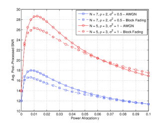
Figure 2: Average post-processed SNR versus choice of power allocation, $\gamma$, for AWGN and block fading.

The difficulty of analytically calculating the above quantity stems from the post-processed SNR having non-linear dependencies on the fading coefficients $h{[1]},\ldots,h{[N]}$. However, it turns out that the optimal $\gamma$ in the i.i.d. Rayleigh block fading case ($\gamma_{0}^{(\rm{fading})}$) is very close to the optimal $\gamma$ in the AWGN case ($\gamma_{0}^{(\rm{AWGN})}$) as derived in [33]. This is displayed in Fig. 2. In Fig. 2, we see that the peaks of both performance curves for block fading (averaged over 15,000 trials) and AWGN noise are quite close together. This is quite beneficial as it is very easy to numerically find the value of $\gamma$ that maximizes the post-processed SNR in the AWGN case, whereas it proves to be much more difficult in the presence of block fading. Because of the proximity of $\gamma_{0}^{(\rm{AWGN})}$ and $\gamma_{0}^{(\rm{fading})}$, we assume that the value of $\gamma$ that maximizes the average post-processed SNR, $\gamma_{0}=\gamma_{0}^{(\rm{AWGN})}\approx\gamma_{0}^{(\rm{fading})}$. The value of $\gamma_{0}$ does, however, change with the blocklength $N$. Furthermore, as the number of transmissions is not necessarily known ahead of time, it is intuitive to not choose $\gamma$ as a function of blocklength. Alternatively, we can fix $\gamma$ based on a reasonable number of packet retransmissions—this is discussed in the following example.

Example 1

To illustrate the performance of the linear feedback scheme, we now provide some simulations. In this first plot (Fig. 3a), the post-processed SNR of the scheme is plotted in contrast to MRC. MRC is analogous to using our scheme but setting $\gamma=0$. In other words, the source simply repeats the packet at each retransmission. Then, retransmissions are combined using a linear receiver similar to the one in (15). The simulations were run with an average transmit power of $\rho=3$ and for both noiseless COI feedback and varying levels of noisy COI feedback. As can be seen, the linear feedback outperforms MRC with a gap that increases with decreasing feedback noise.

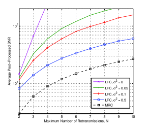
(a) Average Post-processed SNR

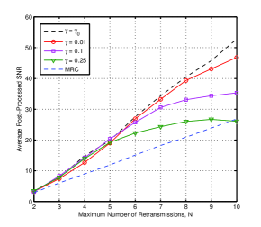
(b) Power Allocation

Figure 3: (a) Average post-processed SNR performance of linear feedback combining (LFC) versus maximal ratio combining. (b) Average post-processed SNR performance of linear feedback combining using different values of $\gamma$.

As mentioned above, $\gamma_{0}$ changes with blocklength, $N$, and therefore should be chosen appropriately. However, in hybrid-ARQ, the required number of retransmissions is often not known ahead of time. Despite this fact, not having this knowledge a priori provides very little penalty to performance. If the number of retransmissions is not assumed to be predetermined, $\gamma$ can be approximately chosen using the feedback noise variance $\sigma^{2}$ and the average transmit power $\rho$. The next figure, Fig. 3b, illustrates the effect of fixing $\gamma$. As is illustrated, fixing $\gamma$ with respect to blocklength yields little performance degradation as long as $\gamma$ is chosen appropriately. The average post-processed SNR for $\gamma=0.01$ performs very close to the scheme when using $\gamma_{0}$ from Fig. 2. Note that Fig. 3b has been plotted on a linear scale to help display the comparison.

IV Multiple Antenna Scenarios

In this section, we show how the feedback scheme for SISO systems can be implemented in both MISO and MIMO systems with current CSI at the source. In addition, an extension of the scheme is given for MIMO systems with perfect COI and only outdated CSI at the source. However, first we look at a MISO system with current quantized CSI along with perfect COI available at the source.

IV-A MISO with Current, Quantized Channel State Information at the Source

Consider a MISO discrete-time system (Fig. 4) with $M_{t}$ transmit antennas and only one receive antenna, where the received packet, ${\mathbf{y}}[k]\in\mathbb{C}^{1\times L}$ is given by

$${\mathbf{y}}[k]={\mathbf{h}}^{T}[k]{\mathbf{X}}[k]+{\mathbf{z}}[k],\quad k=1,\ldots N,$$ (24)

where ${\mathbf{h}}[k]\in\mathbb{C}^{M_{t}\times 1}$ is the channel gain vector, ${\mathbf{X}}[k]\in\mathbb{C}^{M_{t}\times L}$ is the transmitted packet matrix where the columns correspond to channel uses and the rows correspond to antennas, and ${\mathbf{z}}[k]\in\mathbb{C}^{1\times L}$ is additive noise during the $k^{th}$ retransmission with distribution ${\mathcal{C}}{\mathcal{N}}(\mathbf{0},{\mathbf{I}})$. Furthermore, the power constraint at the source is given as $E[\mathrm{tr}({\mathbf{X}}^{*}[k]{\mathbf{X}}[k])]\leq L\rho$, and it is assumed that there is perfect CSI at the destination. However, the source no longer has access to perfect CSI. The destination only feeds back the beamforming vector to be used for current packet retransmission. The previous channel quality information (${\mathbf{h}}^{T}[k-1]{\mathbf{w}}[k-1]$) along with the unquantized channel output is also fed back to the source.

Figure 4: System level block diagram for MISO system with quantized CSI and COI feedback. The feedback information can be described as COI (${\mathbf{y}}[k-1]$), channel quality information (${\mathbf{h}}^{T}[k-1]{\mathbf{w}}[k-1]$), and the beamforming vector (${\mathbf{w}}[k]$).

The transmitted packet matrix ${\mathbf{X}}[k]$ is now generated as an outer product by

$${\mathbf{X}}[k]={\mathbf{w}}[k]\widetilde{{\mathbf{x}}}[k],$$ (25)

where ${\mathbf{w}}[k]\in\mathbb{C}^{M_{t}\times 1}$ denotes the unit norm beamforming vector to be used during retransmission $k$ and $\widetilde{{\mathbf{x}}}[k]\in\mathbb{C}^{1\times L}$ is the effective SISO signal during retransmission number $k$. The power constraint on ${\mathbf{X}}[k]$ now is equivalent to

$$E[\mathrm{tr}({\mathbf{X}}^{*}[k]{\mathbf{X}}[k])] = \mathrm{tr}\left(E[\widetilde{{\mathbf{x}}}^{*}[k]{\mathbf{w}}^{*}[k]{\mathbf{w}}[k]\widetilde{{\mathbf{x}}}[k]]\right)$$ (26)

$$= E[|\widetilde{{\mathbf{x}}}[k]|^{2}]$$

$$\leq L\rho.$$

At this point, it is again assumed that $L=1$ for simplicity which reduces ${\mathbf{y}}[k],\widetilde{{\mathbf{x}}}[k]$, and ${\mathbf{z}}[k]$ to scalars $y[k],\widetilde{x}[k]$, and $z[k]$. We now follow the standard model for limited feedback beamforming by constraining the design of beamforming vector ${\mathbf{w}}[k]$ for packet transmission $k$ to a codebook ${\mathcal{F}}[k]$ containing $2^{B}$ unit vectors [1]. We denote the codebook ${\mathcal{F}}[k]$ as

$${\mathcal{F}}[k]=\left\{{\mathbf{f}}_{1}[k],\ldots,{\mathbf{f}}_{2^{B}}[k]\right\},\quad\lVert{\mathbf{f}}_{j}[k]\rVert=1,1\leq j\leq 2^{B}.$$ (27)

We can use any scheme available in literature to generate the unit beamforming vectors including random vector quantization (RVQ) [39], [40] and Grassmannian line packing [41, 42]. This codebook is accessible to both the source and destination simultaneously. For RVQ, there must be a random seed that is made available to both the source and destination before the communication starts.

The destination decides on the beamforming vector that the source uses during the $k^{th}$ retransmission by solving the following channel quality maximization problem

$${\mathbf{w}}[k]=\mathop{\mathrm{argmax}}_{{\mathbf{f}}_{j}[k]\in{\mathcal{F}}[k]}\left|{\mathbf{h}}^{T}[k]{\mathbf{f}}_{j}[k]\right|^{2}.$$ (28)

Effectively, the destination chooses the unit vector ${\mathbf{w}}[k]$ in the codebook ${\mathcal{F}}[k]$ along which the channel vector ${\mathbf{h}}[k]$ has the largest projection. The information about ${\mathbf{w}}[k]$ is conveyed back to the source in just $B$ bits. The limited feedback capacity ($C_{\rm{LF}}$) for a given codebook design $\{{\mathcal{F}}[k]\}_{k=1}^{\infty}$ can be expressed by

$$C_{\rm{LF}}=E\left[\max_{{\mathbf{f}}_{j}[k]\in{\mathcal{F}}[k]}\log_{2}(1+\rho|{\mathbf{h}}^{T}[k]{\mathbf{f}}_{j}[k]|^{2})\right].$$ (29)

Using the monotonicity of the logarithmic function, $C_{\rm{LF}}$ can be simplified to

$$C_{\rm{LF}} = E\left[\log_{2}(1+\rho\max_{{\mathbf{f}}_{j}[k]\in{\mathcal{F}}[k]}|{\mathbf{h}}^{T}[k]{\mathbf{f}}_{j}[k]|^{2})\right]$$ (30)

$$= E\left[\log_{2}(1+\rho|{\mathbf{h}}^{T}[k]{\mathbf{w}}[k]|^{2})\right].$$

As the number of feedback bits $B$ approach infinity, $C_{\rm{LF}}\rightarrow C_{\rm{MISO}}$, where $C_{\rm{MISO}}=E\left[\log_{2}(1+\rho\lVert{\mathbf{h}}\rVert^{2})\right]$. This is because limited CSI feedback becomes perfect CSI feedback for any codebook design with an infinite number of feedback bits. With the selection of beamforming vector ${\mathbf{w}}[k]$ as described above and packet length $L=1$, the received signal $y[k]$ is given as

$$y[k]={\mathbf{h}}^{T}[k]{\mathbf{w}}[k]\widetilde{x}[k]+z[k],\quad k=1,\ldots N.$$

Pre-multiplying the received signal ${\mathbf{y}}[k]$ by $e^{-j\angle{\mathbf{h}}^{T}[k]{\mathbf{w}}[k]}$, we obtain

$$\widetilde{y}[k]=\left|{\mathbf{h}}^{T}[k]{\mathbf{w}}[k]\right|\widetilde{x}[k]+\widetilde{z}[k],\quad k=1,\ldots N,$$

where $\widetilde{y}[k]=y[k]e^{-j\angle{\mathbf{h}}^{T}[k]{\mathbf{w}}[k]}$ and $\widetilde{z}[k]$ is distributed as ${\mathcal{C}}{\mathcal{N}}(0,1)$. If we let $\widetilde{\lambda}[k]=|{\mathbf{h}}^{T}[k]{\mathbf{w}}[k]|$, we get the overall system in (24) as

$$\widetilde{y}[k]=\widetilde{\lambda}[k]\widetilde{x}[k]+\widetilde{z}[k],\quad k=1,\ldots N,$$ (31)

Finally, gathering all packet retransmissions together as in (3), we can rewrite (31) as

$$\widetilde{{\mathbf{y}}}=\widetilde{{\mathbf{\Lambda}}}\widetilde{{\mathbf{x}}}+\widetilde{{\mathbf{z}}},$$ (32)

where $\widetilde{{\mathbf{\Lambda}}}=\mathrm{diag}(\widetilde{\lambda}[1],\widetilde{\lambda}[2],\ldots,\widetilde{\lambda}[N])$. With this formulation, the MISO system is equivalent to the SISO system in (3); therefore, the SISO scheme can be implemented by replacing the role of $h[k]$ with $\widetilde{\lambda}[k]$ (see Fig. 4).

It can be proven in a similar way to Lemma 1 that the MISO scheme meets the average power constraint. Also, it can be shown that if the feedback channel is perfect, the MISO scheme achieves the capacity of the channel and obtains a doubly exponential decay in error probability. However, to avoid redundancy, this proof is only given for the MIMO case in the next section (Lemma 4). The effects of using different vector quantization techniques and the overall performance of the MISO scheme are now presented in an example.

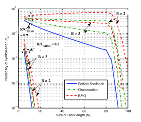
Figure 5: Variation of probability of error with the number of retransmissions for i.i.d. Rayleigh fading at $\rho=0$ dB and $M_{t}=2$. The performance of RVQ, Grassmanian line packing, and perfect feedback are compared for $R/C_{\rm{MISO}}=0.5$ and $R/C_{\rm{MISO}}=0.9$ with $B=2$ and $B=3$.

Example 2

To illustrate the potential of our scheme, consider a MISO system communicating over an i.i.d. Rayleigh block fading channel with each entry of ${\mathbf{h}}[k]$ distributed as ${\mathcal{C}}{\mathcal{N}}({0,1})$. In this example, the COI feedback is assumed to be noiseless (i.e., $\sigma^{2}=0$). Using a limited CSI feedback framework, Fig. 5 plots the packet probability of error curves against the number of retransmissions for two different normalized rates of $0.5$ and $0.9$ where normalized rate is the ratio of the rate of transmission to the channel capacity ($R/C_{\rm{MISO}}$). The plots are for $\rho=0$ dB with a two-antenna source averaged over $10^{6}$ i.i.d. fading realizations. The doubly exponential decay of the curves are clearly visible for all the feedback schemes: perfect CSI feedback and quantized CSI feedback – RVQ and Grassmanian line packing. Even with quantized CSI feedback and moderate normalized rate of $0.5$, only a few retransmissions are required to achieve a very low packet error rate of $1\%$ for both RVQ and Grassmanian line packing.

IV-B MIMO with Current Channel State Information at the Source

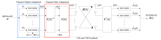
Figure 6: System level block diagram when channel state is known perfectly at both the source and destination.

Consider now a MIMO packet retransmission system (Fig. 6) with $M_{t}$ transmit antennas and $M_{r}$ receive antennas where the number of spatial channels available is $M=\min(M_{r},M_{t})$. The received matrix, ${\mathbf{Y}}[k]\in\mathbb{C}^{M_{r}\times L}$, is given by

$${\mathbf{Y}}[k]={\mathbf{H}}[k]{\mathbf{X}}[k]+{\mathbf{Z}}[k],$$ (33)

where ${\mathbf{X}}[k]\in\mathbb{C}^{M_{t}\times L}$ is, as in MISO, the transmit packet matrix, ${\mathbf{H}}[k]\in\mathbb{C}^{M_{r}\times M_{t}}$ is the block Rayleigh fading channel matrix whose entries are i.i.d. zero-mean complex Gaussian random variables with unit variance, and ${\mathbf{Z}}[k]\in\mathbb{C}^{M_{r}\times L}$ is an additive noise matrix with i.i.d. zero-mean complex Gaussian entries with unit variance. Note that due to the availability of multiple spatial channels, the total packet length has increased to contain $ML$ symbols with $M$ symbols transmitted over each channel use. Again, for the sake of simplicity, we assume that $L=1$ which reduces ${\mathbf{Y}}[k],{\mathbf{X}}[k],$ and ${\mathbf{Z}}[k]$ to column vectors $\vec{{\mathbf{y}}}[k],\vec{{\mathbf{x}}}[k],$ and $\vec{{\mathbf{z}}}[k]$. When the current block fading matrix is known both at the source and destination, we can effectively diagonalize the channel. Let

$${\mathbf{H}}[k]={\mathbf{U}}[k]\mathbf{\Lambda}[k]{\mathbf{V}}^{*}[k],$$ (34)

be a compact singular value decomposition (SVD) of the channel matrix ${\mathbf{H}}[k]$, where ${\mathbf{U}}[k]\in{\mathbb{C}}^{M_{r}\times M},\mathbf{\Lambda}[k]\in{\mathbb{C}}^{M\times M},$ and ${\mathbf{V}}[k]\in{\mathbb{C}}^{M_{t}\times M},$ with

$$\mathbf{\Lambda}[k]=\mathrm{diag}\left(\lambda_{1}[k],\ldots,\lambda_{M}[k]\right),\quad\lambda_{1}[k]\geq\lambda_{2}[k]\ldots\geq\lambda_{M}[k]\geq 0,$$ (35)

$${\mathbf{U}}^{*}[k]{\mathbf{U}}[k]={\mathbf{V}}^{*}[k]{\mathbf{V}}[k]={\mathbf{I}}.$$ (36)

We can design the source vector $\vec{{\mathbf{x}}}[k]$ as

$$\vec{{\mathbf{x}}}[k]={\mathbf{V}}[k]{\mathbf{s}}[k],$$ (37)

where ${\mathbf{s}}[k]\in\mathbb{C}^{M\times 1}$ with ${\mathbf{V}}[k]$ defined by (34) and (36). Also pre-multiplying the received vector by ${\mathbf{U}}^{*}[k]$, we obtain the effective system described by (33) as

$${\mathbf{U}}^{*}[k]\vec{{\mathbf{y}}}[k] = {\mathbf{U}}^{*}[k]{\mathbf{H}}[k]{\mathbf{V}}[k]{\mathbf{s}}[k]+{\mathbf{U}}^{*}[k]\vec{{\mathbf{z}}}[k]$$

$$\widetilde{{\mathbf{y}}}[k] = \mathbf{\Lambda}[k]{\mathbf{s}}[k]+\widetilde{{\mathbf{z}}}[k],$$ (38)

where $\widetilde{{\mathbf{y}}}[k]\in{\mathbb{C}}^{M\times 1}$ and $\widetilde{{\mathbf{z}}}[k]\in{\mathbb{C}}^{M\times 1}$. The effective noise $\widetilde{{\mathbf{z}}}[k]$ is distributed as $\mathcal{CN}({\bf 0},{\mathbf{I}})$ due to the rotational invariance of complex i.i.d. Gaussian vectors. Due to the a priori knowledge of the channel at the source, spatial waterfilling can be performed across the $M$ parallel spatial channels for each packet transmitted. The entries of the waterfilling matrix $\mathbf{\Xi}[k]=\textrm{diag}\left(\xi_{1}[k],\ldots,\xi_{M}[k]\right)$ are defined as

$$\xi_{i}[k]=\max\left(0,\frac{1}{\xi_{0}[k]}-\frac{1}{{\lambda^{2}_{i}}[k]}\right),\quad 1\leq i\leq M.$$ (39)

The value of the constant $\xi_{0}[k]$ is the water-filling level chosen to satisfy the power constraint

$$\sum_{i=1}^{M}\xi_{i}[k]=1.$$ (40)

Furthermore, the capacity $C_{\rm{TR}}$ of a MIMO channel with the fading matrix known both at the source and destination can be written as

$$C_{\rm{TR}}=\sum_{i=1}^{M}E\left[\log_{2}(1+\rho\xi_{i}{\lambda}_{i}^{2})\right],$$ (41)

where we have dropped the retransmission index $k$ due to the i.i.d. nature of the block fading matrix. With current CSI at the source and destination, the overall channel capacity of the MIMO channel can be expressed as a sum of $M$ parallel non-interfering SISO spatial channels each with capacity $C_{i}$ where $C_{i}=E\left[\log_{2}(1+\rho\xi_{i}{\lambda}_{i}^{2})\right],\quad 1\leq i\leq M.$

With the aid of the waterfilling matrix defined in (39), (38) can now be written as

$$\widetilde{{\mathbf{y}}}[k] = {\mathbf{\Lambda}}[k]\mathbf{\Xi}[k]^{1/2}\widetilde{{{\mathbf{x}}}}[k]+\widetilde{{\mathbf{z}}}[k],$$

where ${\mathbf{s}}[k]=\mathbf{\Xi}[k]^{1/2}\widetilde{{{\mathbf{x}}}}[k]$. Note that the spatial waterfilling (or power adaptation) does not make use of the COI fed back to the source at all. Letting $\widetilde{\mathbf{\Lambda}}[k]={\mathbf{\Lambda}}[k]\mathbf{\Xi}[k]^{1/2}$, the overall system can be represented in matrix form as

$$\widetilde{{\mathbf{y}}}[k]=\widetilde{\mathbf{\Lambda}}[k]\widetilde{{{\mathbf{x}}}}[k]+\widetilde{{\mathbf{z}}}[k].$$ (42)

We next transmit $M$ symbols over $M$ parallel spatial channels by exploiting the COI and previous CSI available at the source using a maximum of $N$ transmissions. In other words, with (42), we can implement $M$ parallel instances of the COI feedback SISO scheme—one for each spatial channel. Similar to the MISO case, we replace the role of $h[k]$ with $\widetilde{\lambda}_{i}[k]$ for the $i^{th}$ spatial channel.

It is quite possible that each of the source constellations $\varTheta_{i}[N]$ has a different number of constellation points; note that $\varTheta_{i}[N]$ denotes the source constellation used for the $i^{th}$ spatial channel. The number of equally likely constellation points chosen for each channel depends on the spatial capacity $C_{i}$ of the subchannel. Therefore, the number of constellations points must be less than $2^{NC_{i}}$.

The overall schematic of the proposed scheme, shown in Fig. 6, clearly demonstrates the independent constellation mapping of each of the $M$ symbols of packet ${\boldsymbol{\theta}}$ along with the separation of the channel output adaptation from current channel state adaptation. Furthermore, it can be shown that, if the feedback channel is perfect, any rate less than capacity can be achieved by the above scheme at doubly exponential rate.

Lemma 4.

If $\sigma^{2}=0$, the proposed scheme achieves any rate $R<C_{\rm{TR}}$. Viewing the rate $R$ as a sum of $M$ spatial channel rates, $R=\sum_{i=1}^{M}R_{i},$ the coding scheme can achieve any rate $R_{i}<C_{i}$ for the $i^{th}$ spatial channel. Furthermore the probability of error ($P_{e}$) for the packet decays doubly exponentially as the function of the number of transmissions $N$. In other words, for sufficiently large $N$,

$$P_{e}\leq\beta_{1}\exp\left(-2^{(N\beta_{2}+\beta_{3})}\right),$$

where $\beta_{1}$ and $\beta_{2}$ are positive constants, while $\beta_{3}$ is a real constant for a given rate $R$.

Proof.

See Appendix. ∎

IV-C MIMO with Outdated Channel State Information at the Source

In the case when there are multiple antennas at both the source and destination and the source has access to only outdated CSI, a direct extension of the SISO scheme for perfect COI (Lemma 2) can be made. Using the same system setup as in (33), if $L=1$, we can write the feedback scheme recursively as

$$\vec{{\mathbf{x}}}[k+1] = \left({\mathbf{I}}+\rho{\mathbf{H}}^{*}[k]{\mathbf{H}}[k]\right)^{-1/2}\left(\vec{{\mathbf{x}}}[k]-\rho{\mathbf{H}}^{*}[k]\vec{{\mathbf{z}}}[k]\right)$$ (43)

$$\widehat{{\textrm{{\boldmath{$\theta$}}}}}[k] = \left({\mathbf{I}}-\mathbf{\Phi}[k]\mathbf{\Phi}^{*}[k]\right)\textrm{{\boldmath{$\theta$}}}+\rho\mathbf{\Phi}[k]\mathbf{\Phi}^{*}[k]\sum_{m=1}^{k}(\mathbf{\Phi}^{-1}[m-1])^{*}{\mathbf{H}}^{*}[m]\vec{{\mathbf{z}}}[m],$$ (44)

where

$$\mathbf{\Phi}[k]=\left({\mathbf{I}}+M\rho{\mathbf{H}}^{*}[1]{\mathbf{H}}[1]\right)^{-1/2}\cdots\left({\mathbf{I}}+M\rho{\mathbf{H}}^{*}[k]{\mathbf{H}}[k]\right)^{-1/2}.$$ (45)

Unfortunately, even if the feedback channel is perfect but only outdated CSI is available at the source, it is difficult to prove a result similar to Lemma 4. Although it can be shown for some positive rates a doubly exponential decay of probability of error is achievable, it has not been proven for all rates below capacity. We now broaden our focus back to the view of the whole hybrid-ARQ scheme in the next section.

V The Hybrid-ARQ Scheme and Variations

Rather than focusing on the packet estimate, $\widehat{{\boldsymbol{\theta}}}[k]$, we now consider the overall hybrid-ARQ scheme including the FEC. For the FEC, we assume the use of a systematic turbo code; although, any systematic block code can work. Because of this choice, we will perform only soft decoding at the output of the packet combining step. This means for each symbol in the estimated packet, $\widehat{\theta}_{i}[k]$, we will form a set of log-likelihood ratios as

$$LLR_{i}=\left\{\log\left[\frac{p(\theta_{i}=\psi_{j}|\hat{\theta}_{i}[k])}{\sum_{\ell\neq j}p(\theta_{i}=\psi_{\ell}|\hat{\theta}_{i}[k])}\right]:j=1,2,\ldots,\left|\Theta[N]\right|\right\},$$ (46)

where $\psi_{j}$ for $j=1,2,\ldots,\left|\Theta[N]\right|$ are the points of the constellation $\Theta[N]$ utilized for modulation. Upon calculating these sets, they are then passed to the turbo decoder for decoding. The specific turbo code implemented is a rate $L_{\textrm{info}}/L_{\textrm{coded}}=1/3$ turbo code defined in the UMTS standard; more details are given in the Simulations section.

Now, we introduce different configurations of the overall scheme that might help adapt to different circumstances (e.g., feedback link rate, transmit/receive duration, etc.). To do so, we look at varying the amount of COI feedback sent to the source; this is also done to illustrate the trade-off between performance (e.g., throughput, FER, etc.) and the amount of information fed back. Note that the case of CSI-only feedback has already been explored in the literature; see for example [2, 3, 27, 28, 29]. Therefore the emphasis here is in varying the amount of COI feedback.

The most straightforward of the possible COI feedback configurations is one where the destination simply feeds back everything it receives without discrimination. This utilizes a noiseless/noisy version of the full received packet for feedback information; hence, we will refer to this method as full packet feedback (FPF). Alternatively, one can alter FPF by implementing a well-known concept in hybrid-ARQ with feedback [31]; instead of feeding back all the symbols of the received packet, we can instead feed back only the $T$ “least reliable” symbols with their indices. The measure of “reliability” can be based off metrics such as the log-likelihood ratio (LLR) or the logarithm of the a posteriori probabilities (log-APP) [32]. Since only some of the symbols in the packet are fed back, we will refer to this scheme as partial packet feedback (PPF).

V-A Full Packet Feedback (FPF)

In FPF, we propose a hybrid-ARQ scheme where the source is assumed to have access to a noiseless/noisy version of the last received packet. The performance of the perfect COI feedback scenario is used to demonstrate the maximum possible gains that can be achieved with the addition of channel output feedback. To help explicitly show the feedback information available, we now introduce ${\mathbf{r}}[k]$ as the channel output feedback side-information available at the source at packet transmission $k$. In FPF,

$${\mathbf{r}}[k]={\mathbf{y}}[k-1]+{\mathbf{n}}[k-1],$$ (47)

where, in this case, ${\mathbf{r}}[k]\in\mathbb{C}^{1\times L}$.

As mentioned before, the first transmission of packet $\theta$ is assumed to be a codeword of a FEC code. If a NACK is received at the source, each subsequent packet is encoded symbol-wise by the linear feedback code described in Section III. This is used to refine the destination’s estimate of each symbol in the original packet. To display the performance of the scheme, we look at comparing the normalized throughput of this scheme with the turbo-coded hybrid-ARQ used in [34]. This standard uses a rate-compatible punctured turbo code to encode the packet. Specifically, it uses a rate 1/3 UMTS turbo code [43] and then punctures it for use in hybrid-ARQ. If sending one packet and $M$ spatial channels are available for the MIMO setting, the assignment of $M$ symbols for $M$ spatial channels is done arbitrarily. Note that it is plausible that using dynamic adaptive modulation for each of the spatial channels or coordinating multiple retransmissions[2] might result in improvement in throughput. However, we do not consider this here, but we point out that in most of the cases our proposed scheme can be combined with the innovations on using CSI more efficiently.

V-B Partial Packet Feedback (PPF)

For sake of practicality, it is desirable to minimize the amount of COI feedback information needed to be sent back to the source. As a step towards this, we now look at the effects of limiting the size of the COI feedback packet. We try to utilize the limited feedback channel in the most useful way by feeding back not the complete packet but only relatively few of the symbols in the received packet. As mentioned above, in the partial packet mode, the choice of COI feedback information is based on the relative reliability of soft decoded bits. This addition to the scheme is motivated by the technique used in [32] where it was shown that focusing on the least reliable information bits can greatly improve the performance of turbo-coded hybrid-ARQ. The selection process to construct the feedback packet, ${\mathbf{r}}[k]$, is performed at the destination using the following method. The received packet ${\mathbf{y}}[k]$ (or ${\mathbf{Y}}[k]$ as in (33)) is combined with the $k-1$ previous received packets using MRC in the case of Chase combining or as described above if linear COI feedback coding is employed. After combining, the destination now has an estimate of the desired packet, $\widehat{{\boldsymbol{\theta}}}[k]$. This packet estimate is now passed on to the turbo decoder, and its corresponding output is a set of LLRs for each original information bit. For notation, we refer to the LLR produced by the turbo decoder for the $i^{th}$ information bit, $m_{i}$, as $\ell_{i}$, which can be mathematically written as

$$\ell_{i}=\log\left[\frac{p(m_{i}=0|{\mathbf{y}}[1])}{p(m_{i}=1|{\mathbf{y}}[1])}\right],\quad 1\leq i\leq L_{\rm info}.$$ (48)

The least reliable bits are chosen as the $T$ bits whose LLR values have the smallest magnitude, i.e., $|\ell_{i}|<\ell_{\rm th},$ where $\ell_{\rm th}$ is chosen appropriately. The magnitude of $\ell_{i}$ close to zero indicates that the bit is almost equally likely to be either a 1 or a 0. Then, the set of symbols whose realizations are to be fed back is

$$I_{\rm{sym}}=\left\{\theta_{k}:m_{i}\in\theta_{k}\textrm{ and }|\ell_{i}|<\ell_{\rm th},\quad 1\leq i\leq L_{\rm{info}},\quad 1\leq k\leq L\right\},$$ (49)

meaning the symbol is chosen to be fed back if it contains one of the least reliable information bits. Let $|I_{\rm sym}|=T_{\rm sym}$. With this technique, we can then write the feedback packet, ${\mathbf{r}}_{T}[k]$, as

$${\mathbf{r}}_{T}[k]={\mathbf{y}}_{T}[k-1]+{\mathbf{n}}_{T}[k-1],$$ (50)

where

$${\mathbf{y}}_{T}[k-1]=\left\{y_{i}[k-1]:\theta_{i}\in I_{\rm{sym}}\right\}.$$ (51)

Since $T_{\rm sym}$ channel outputs are being fed back, ${\mathbf{n}}_{T}[k]$ is of length $T_{\rm sym}$. Note that the selection process is straightforward in this case because we assume the use of a systematic turbo code. It is also important to note that the $T_{\rm sym}$ symbols are chosen only once (after the first transmission). This process can be done after each retransmission but would require more feedback resources. Finally, if it is assumed that the number of channel uses per packet retransmission are constant, one can fill in the remaining $L-T_{\rm sym}$ channel uses in numerous ways. One particular way is what we will refer to as partial packet feedback with partial Chase combining (PPF-PC). In this mode, on the forward transmission, the new $T_{\rm sym}$ symbols generated for the $T_{\rm sym}$ least reliable symbols based on our linear coding scheme are sent in conjunction with the repetition of the remaining $(L-T_{\rm sym})$ other symbols used for Chase combining.

VI Simulations

In this section we present numerical simulations to demonstrate the improvements possible with inclusion of our proposed linear COI feedback coding in hybrid-ARQ schemes. We assume that the channel is i.i.d. Rayleigh block fading. We limit the number of retransmissions to a maximum of four (i.e., $N=4$). All the throughput calculations are done by averaging over $10^{3}$ new packet transmissions.

The metric defined for calculating normalized throughput is given as:

$$\tau=\frac{1}{E[B]},$$

where $1\leq B\leq N$ is the number of transmissions needed for successful decoding of a packet ${\boldsymbol{\theta}}$. This can be equivalently thought of as a packet success rate or the inverse of the average number of packets needed for successful transmission. If the number of retransmissions reaches the maximum number before successful decoding, the throughput contribution is zero. Note that this metric is meaningful only when comparing constant-length packet schemes. Also the above throughput definition implies that as $\rho\rightarrow\infty,\tau\rightarrow 1$ for all the protocols; including Chase and our proposed scheme.

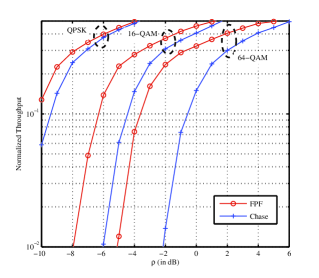
(a) MIMO Channel

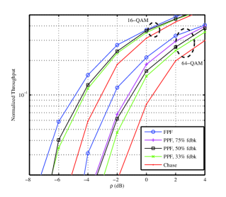
(b) Partial Packet Feedback

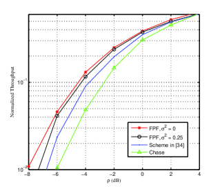
(c) Partial COI

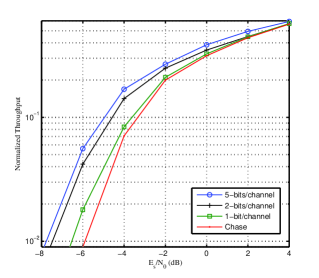
(d) Quantized COI

Figure 7: (a) Plot of variation of throughput for FPF and Chase combining with channel SNR $\rho$ for $2\times 2$ MIMO channel. The performance is compared for QPSK, 16-QAM and 64-QAM constellations with $L_{\rm{info}}M=2020$ bits. (b) Plot of variation of throughput for PPF and Chase combining with channel SNR $\rho$ for a SISO channel. The amount of PPF feedback is varied from $33\%$ to $75\%$ of the total frame size. The performance is compared for 16-QAM and 64-QAM with $L_{\rm{info}}=2020$ bits. (c) Plot of variation of throughput for FPF with noisy feedback against Chase combining and HSDPA for a SISO channel. The performance is compared for QPSK constellation with $L_{\rm{info}}=3200$ bits. (d) Plot of variation of throughput for FPF with quantized COI feedback against Chase combining for a SISO channel. The performance is compared for 16-QAM constellation with $L_{\rm{info}}=2020$ bits.

Fig. 7a compares the performance of FPF scheme with perfect COI feedback against Chase combining for QPSK, 16-QAM, and 64-QAM constellations over a $2\times 2$ MIMO channel. The FEC code used for simulations is a 1/3 UMTS turbo code with eight decoding iterations. It is seen that most of the gains from our proposed scheme are realized in the low SNR regime. The FPF for QPSK displays gains of around 1 dB over Chase combining, and in 16-QAM, it gives an improvement of about 2 dB over Chase combining. Furthermore, the gain increases to 3 dB when the denser constellation of 64-QAM is chosen. It should be noted that these gains have been realized directly at the packet level and not at the bit level. This shows that with four retransmissions the power required at the source can be halved with the inclusion of the proposed linear coding scheme.

In Fig. 7b, we plot the normalized throughput for PPF-PC for perfect COI feedback against traditional Chase combining scheme for 16-QAM and 64-QAM over a SISO channel. The amount of COI feedback symbols from the destination to the source is varied from $33\%$ to $75\%$ of the total feedforward packet size. For 64-QAM with a 1/3 UMTS turbo code and $L_{\rm info}=2020$, the length of the packet is $L=1010$ symbols. Therefore the number of feedback symbols $T$ for 64-QAM is varied from $T=337$ to $T=757$. Again we can see the improvements for 16-QAM and 64-QAM. Although the gains are smaller than the ones for full packet feedback, they are still significant. It is actually interesting to note that in 16-QAM most of the improvement in performance is reached with only $50\%$ of COI feedback information. With $33\%$ COI feedback, PPF scheme still shows an improvement of 1 dB over Chase for 16-QAM and a substantial improvement of 2 dB for 64-QAM constellation.

Fig. 7c compares the normalized throughput for FPF with noisy COI feedback against Chase combining and the scheme in [34]. It is seen that even with a noise of $\sigma^{2}=0.25$ on the channel output feedback channel, we see an improvement of about $0.5$ dB for the linear feedback scheme over the scheme in [34] in the low SNR regime. Furthermore this gain is realized with only the addition of a very low complexity linear coder at source and destination.

Finally, Fig. 7d compares the normalized throughput for FPF with quantized COI feedback for 16-QAM constellation. At the destination, each of the components – inphase and quardature phase, are quantized using certain number of bits and then mapped to the QAM constellation. It is seen that even with 1-bit of quantization per phase leads to improvement in the performance over the conventional Chase combining. However, most of the gains are obtained for 5-bits per phase of quantization.

VII Conclusions

In this paper, we have investigated a new hybrid-ARQ scheme that utilizes COI feedback side-information from the destination. This is motivated by trying to close the performance gap between Chase combining and incremental redundancy using feedback in order to leverage the implementation savings of a Chase combining system [44]. In normal Chase combining, packets are combined using maximum ratio combining (MRC); however, the proposed scheme incorporates feedback by combining the packets using a linear feedback code for fading channels with noisy feedback. Note that this also includes a new encoding step. It was shown through Monte Carlo simulations that the post-processed SNR performance of the linear feedback scheme greatly outperforms that of regular MRC. In addition, since the code is built on linear operations, it adds little complexity to the overall packet encoder and decoder assuming feedback side information is present. The full hybrid-ARQ scheme was analyzed using two main modes of operation: full packet feedback (FPF) in which the source was assumed to have access to a noiseless/noisy version of the last received packet and partial packet feedback (PPF) in which only a subset of the received symbol are fed back to the source. Simulations show that the addition of feedback to hybrid-ARQ greatly increases the performance and outperforms incremental redundancy in most cases.

-A Proof of Lemma 2

Proof.

The encoding for perfect COI feedback using (9) can be written for each $x[k]$ as

$$x[k+1]=\phi^{-1}[k]e[k],$$ (52)

where

$$e[k] = \theta-\widehat{\theta}[k].$$ (53)

The operations at the decoder side can also be given by

$$\widehat{x}[k+1] = \left(1+\rho h^{*}[k+1]h[k+1]\right)^{-1}\rho h^{*}[k+1]y[k+1],$$ (54)

$$\widehat{e}[k] = \phi[k]\widehat{x}[k+1],$$ (55)

$$\widehat{{\theta}}[k+1] = \widehat{{\theta}}[k]+\widehat{e}[k].$$ (56)

For initialization purposes, it is assumed that $\widehat{\theta}[0]=0$. It can be seen from (53) and (56), that the error, $e[k]$, for the symbol $\theta$ satisfies the relation

$$e[k+1]=e[k]-\widehat{e}[k].$$ (57)

Then, implementing (52) and (57), we can rewrite $x[k+1]$ as

$$x[k+1] = \phi^{-1}[k]\left(e[k-1]-\widehat{e}[k-1]\right)$$

$$= \phi^{-1}[k]\left(\phi[k-1]x[k]-\phi[k-1]\widehat{x}[k]\right)$$

$$= \left(1+\rho|h[k]|^{2}\right)^{1/2}(x[k]-\widehat{x}[k])$$

$$= \left(1+\rho|h[k]|^{2}\right)^{-1/2}\left(x[k]-\rho h^{*}[k]z[k]\right).$$

According to (52),

$$\theta-\widehat{{\theta}}[k] = \phi[k]x[k+1]$$

$$= \phi[k]\left(1+\rho|h[k]|^{2}\right)^{-1/2}\left(x[k]-\rho h^{*}[k]z[k]\right)$$

$$= \phi[k]\left(1+\rho|h[k]|^{2}\right)^{-1/2}x[k]-\rho\phi[k]\left(1+\rho|h[k]|^{2}\right)^{-1/2}h^{*}[k]z[k]$$

$$= |\phi[k]|^{2}\theta-\rho|\phi[k]|^{2}\sum_{m=1}^{k}\phi^{-1}[m-1]h^{*}[m]z[m].$$

Therefore, it follows that

$$\widehat{{\theta}}[k]=\left(1-|\phi[k]|^{2}\right)\theta+\rho|\phi[k]|^{2}\sum_{m=1}^{k}\phi^{-1}[m-1]h^{*}[m]z[m].$$

∎

-B Proof of Lemma 4

Proof.

We present the proof for $L=1$. The generalization of it immediately follows. For the $i^{th}$ spatial channel, we select the symbol $\theta_{i}$ from a square QAM constellation consisting of $M_{i}[N]=2^{NR_{i}}$ symbols. According to the recursive definition in Lemma 2, the $i^{th}$ spatial signal is given as

$$\widetilde{x}_{i}[k]=\prod_{l=1}^{k-1}\frac{1}{\sqrt{1+\rho\widetilde{\lambda}^{2}_{i}[l]}}\theta_{i}-\rho\sum_{m=1}^{k-1}\left(\prod_{l=m}^{k-1}\frac{1}{\sqrt{1+\rho\widetilde{\lambda}^{2}_{i}[l]}}\right)\widetilde{\lambda}_{i}[m]\widetilde{z}_{i}[m].$$ (58)

Let

$$\widetilde{\phi}_{i}[k]=\prod_{l=1}^{k}\frac{1}{\sqrt{1+\rho\widetilde{\lambda}^{2}_{i}[l]}},\quad\widetilde{\phi}_{i}[0]=1.$$ (59)

Now (58) can be rewritten as

$$\widetilde{x}_{i}[k]=\widetilde{\phi}_{i}[k-1]\left(\theta_{i}-\rho\sum_{m=1}^{k-1}\frac{\widetilde{\lambda}_{i}[m]\widetilde{z}_{i}[m]}{\widetilde{\phi}_{i}[m-1]}\right).$$ (60)

Based on (14) which describes the unbiased estimation algorithm at the destination,

$$\widehat{\theta}^{u}_{i}[N]=\theta_{i}+\rho\frac{\widetilde{\phi}_{i}^{2}[N]}{1-\widetilde{\phi}_{i}^{2}[N]}\sum_{k=1}^{N}\frac{\widetilde{\lambda}_{i}[k]}{\widetilde{\phi}_{i}[k-1]}\widetilde{z}_{i}[k].$$ (61)

Let

$$e^{u}_{i}[N] = \widehat{\theta}_{i}[N]-\theta_{i}.$$

Given channel realizations over blocklength $N$, $\{{\mathbf{H}}[k]\}_{k=1}^{N}$, and a known $\theta_{i}$, the random variable $e^{u}_{i}[N]$ is just a complex Gaussian random variable with conditional mean

$$E\left[e^{u}_{i}[N]\Big{|}\{{\mathbf{H}}[k]\}_{k=1}^{N},\theta_{i}\right] = E\left[\rho\frac{\widetilde{\phi}_{i}^{2}[N]}{1-\widetilde{\phi}_{i}^{2}[N]}\sum_{k=1}^{N}\frac{\widetilde{\lambda}_{i}[k]}{\widetilde{\phi}_{i}[k-1]}\widetilde{z}_{i}[k]\Big{|}\{{\mathbf{H}}[k]\}_{k=1}^{N},\theta_{i}\right]$$

$$= 0.$$

Similarly for the variance of $e^{u}_{i}[N]$, we obtain

$$\textrm{Var}\left(e^{u}_{i}[N]\Big{|}\{{\mathbf{H}}[k]\}_{k=1}^{N},\theta_{i}\right) = \textrm{Var}\left(\rho\frac{\widetilde{\phi}_{i}^{2}[N]}{1-\widetilde{\phi}_{i}^{2}[N]}\sum_{k=1}^{N}\frac{\widetilde{\lambda}_{i}[k]}{\widetilde{\phi}_{i}[k-1]}\widetilde{z}_{i}[k]\Big{|}\{{\mathbf{H}}[k]\}_{k=1}^{N},\theta_{i}\right)$$ (62)

$$= \rho^{2}\frac{\widetilde{\phi}_{i}^{4}[N]}{(1-\widetilde{\phi}_{i}^{2}[N])^{2}}\sum_{k=1}^{N}\frac{\widetilde{\lambda}^{2}_{i}[k]}{\widetilde{\phi}^{2}_{i}[k-1]}.$$

The symbol $\theta_{i}$ is drawn from a square QAM constellation $\varTheta_{i}[N]$ given by,

$$\varTheta_{i}[N]=\sqrt{\alpha_{i}[N]}\left\{\pm 1\pm 1j,\pm 1\pm 3j,\cdots\cdots,\pm\left(\sqrt{M_{i}[N]}-1\right)\pm\left(\sqrt{M_{i}[N]}-1\right)j\right\},$$ (63)

where the scaling factor $\alpha_{i}[N]$ satisfies the power constraint at the source

$$E[|\theta_{i}|^{2}]=\frac{2}{3}(M_{i}[N]-1)\alpha_{i}[N]=\rho.$$ (64)

A correct decision about $\theta_{i}$ is made by the destination if the error $e^{u}_{i}[N]$ falls within the square ($\Box_{i}[N]$) of length $2\sqrt{\alpha_{i}[N]}$. Let

$$P_{e}\left(\{{\mathbf{H}}[k]\}_{k=1}^{N},\theta_{i}\right)=P\left(e^{u}_{i}[N]\notin\Box_{i}[N]\Big{|}\{{\mathbf{H}}[k]\}_{k=1}^{N},\theta_{i}\right).$$

Clearly,

$$P_{e}\left(\{{\mathbf{H}}[k]\}_{k=1}^{N},\theta_{i}\right) \leq P\left(|\mathfrak{Re}(e^{u}_{i}[N])|>\sqrt{\alpha_{i}[N]}\Big{|}\{{\mathbf{H}}[k]\}_{k=1}^{N},\theta_{i}\right)+$$

$$P\left(|\mathfrak{Im}(e^{u}_{i}[N])|>\sqrt{\alpha_{i}[N]}\Big{|}\{{\mathbf{H}}[k]\}_{k=1}^{N},\theta_{i}\right),$$

where $\mathfrak{Re}(e^{u}_{i}[N])$ and $\mathfrak{Im}(e^{u}_{i}[N])$ denote the real and imaginary part of $e^{u}_{i}[N]$ respectively. Using the identical distribution of the real and imaginary components of the error $e^{u}_{i}[N]$, we get

$$P_{e}\left(\{{\mathbf{H}}[k]\}_{k=1}^{N},\theta_{i}\right)\leq 4Q\left(\sqrt{\frac{{\alpha_{i}[N]}}{{\textrm{Var}\left(\mathfrak{Re}(e^{u}_{i}[N])\Big{|}\{{\mathbf{H}}[k]\}_{k=1}^{N},\theta_{i}\right)}}}\right).$$

Clearly,

$$\textrm{Var}\left(\mathfrak{Re}(e^{u}_{i}[N])\Big{|}\{{\mathbf{H}}[k]\}_{k=1}^{N},\theta_{i}\right)=\frac{1}{2}\textrm{Var}\left(e^{u}_{i}[N]\Big{|}\{{\mathbf{H}}[k]\}_{k=1}^{N},\theta_{i}\right).$$

Therefore,

$$P_{e}\left(\{{\mathbf{H}}[k]\}_{k=1}^{N},\theta_{i}\right) \leq 4Q\left(\sqrt{\frac{3\left(1-\widetilde{\phi}_{i}^{2}[N]\right)^{2}}{(M_{i}[N]-1)\rho\widetilde{\phi}_{i}^{4}[N]\sum_{k=1}^{N}\frac{\widetilde{\lambda}^{2}_{i}[k]}{\widetilde{\phi}^{2}_{i}[k-1]}}}\right)$$ (65)

$$= 4Q(\sqrt{a_{i}[N]}),$$

where

$$a_{i}[N]={\frac{3\left(1-\widetilde{\phi}_{i}^{2}[N]\right)^{2}}{(M_{i}[N]-1)\rho\widetilde{\phi}_{i}^{4}[N]\sum_{k=1}^{N}\frac{\widetilde{\lambda}^{2}_{i}[k]}{\widetilde{\phi}^{2}_{i}[k-1]}}}.$$ (66)

We next show that with probability 1, $a_{i}[N]$ increases at least exponentially with $N$. From the definition of $\widetilde{\phi}_{i}[N]$ in (59) we have $0\leq\widetilde{\phi}_{i}[N]\leq 1,N\geq 0$. Also the definition implies that the sequence $\{\widetilde{\phi}_{i}[N]\}_{N=0}^{\infty}$ is a monotonically decreasing sequence for arbitrary channel matrices. Hence by Theorem $3.14$ in [45], the sequence $\{\widetilde{\phi}_{i}[N]\}_{N=0}^{\infty}$ converges. Also,

$$E[\log_{2}\widetilde{\phi}_{i}[N]] = -\frac{1}{2}\sum_{k=1}^{N}E\left[\log_{2}\left(1+\rho\widetilde{\lambda}_{i}^{2}[k]\right)\right]$$ (67)

$$= -\frac{N}{2}C_{i}$$ (68)

Using (68) and the strong law of large numbers (SLLN), we know that for any given $\epsilon>0,\exists N_{1}$ such that

$$P\left(\left|\frac{1}{N}\log_{2}\widetilde{\phi}_{i}[N]+\frac{1}{2}C_{i}\right|<\frac{\epsilon}{2}C_{i}\right)=1\quad\forall N>N_{1}.$$

In particular,

$$P\left(\widetilde{\phi}_{i}[N]<2^{-\frac{1}{2}N(1-\epsilon)C_{i}}\right)=1\quad\forall N>N_{1}.$$ (69)

By the almost sure convergence of $\{\widetilde{\phi}_{i}[N]\}_{N=0}^{\infty}$ to zero, we can choose $N_{2}$ such that

$$P\left(1-\widetilde{\phi}_{i}^{2}[N]>\frac{1}{\sqrt{3}}\right)=1\quad\forall N>N_{2}.$$ (70)

Using SLLN again, we obtain that for a given $\epsilon>0,\exists N_{3}$ such that

$$P\left(\sum_{k=1}^{N}\widetilde{\lambda}^{2}_{i}[k]<\eta_{i}N(1+\epsilon)\right)=1\quad\forall N>N_{3},$$ (71)

where $\eta_{i}=E[\widetilde{\lambda}^{2}_{i}[k]]$. Substituting the bounds given by (69), (70) and (71) into the expression of $a_{i}[N]$ in (66), we obtain that $\forall N>\max\{N_{1},N_{2},N_{3}\}$ with probability 1,

$$a_{i}[N] \geq \frac{1}{\rho}\frac{3\left(\frac{1}{\sqrt{3}}\right)^{2}}{2^{NR_{i}}2^{-N(1-\epsilon)C_{i}}\eta_{i}N(1+\epsilon)}$$

$$= \frac{1}{\rho}\frac{2^{N\left((1-\epsilon)C_{i}-R_{i}\right)}}{\eta_{i}N(1+\epsilon)}.$$

The positive value $\epsilon$ also satisfies the inequality,

$$\rho\eta_{i}N(1+\epsilon)\leq 2^{\epsilon NC_{i}},\quad\forall N>N_{4}.$$

Clearly it follows that $\forall N>N_{\rm max}$

$$a_{i}[N]\geq 2^{N\left((1-2\epsilon)C_{i}-R_{i}\right)},$$

where $N_{\rm max}=\max\{N_{1},N_{2},N_{3},N_{4}\}$.

Thus, we have shown that with probability one, the input parameter of the $Q$-function increases exponentially. Furthermore it is very well known that $Q$-function decays exponentially and can be bounded by,

$$Q(x)\leq\frac{1}{2}e^{-x^{2}/2},\quad\forall x\geq 0.$$

From the above two equations we immediately obtain,

$$P_{e}\left(\{{\mathbf{H}}[k]\}_{k=1}^{N},\theta_{i}\right)\leq 2e^{-\frac{1}{2}2^{N\left((1-2\epsilon)C_{i}-R_{i}\right)}}.$$

Note that we can choose $\epsilon$ arbitrarily. Picking $\epsilon<\displaystyle\min_{i=1,2,\ldots,M}\textstyle\frac{1}{2}\left(1-\frac{R_{i}}{C_{i}}\right)$ guarantees that the decay is doubly exponential. ∎

References

- [1] D. J. Love, R. W. Heath, Jr., V. K. N. Lau, D. Gesbert, B. D. Rao, and M. Andrews, “An overview of limited feedback in wireless communication systems,” IEEE Jour. Select. Areas in Commun., vol. 26, no. 8, pp. 1341–1365, Oct. 2008.
- [2] H. Sun, J. Manton, and Z. Ding, “Progressive linear precoder optimization for MIMO packet retransmissions,” IEEE Jour. Select. Areas in Commun., vol. 24, no. 3, pp. 448–456, Mar. 2006.
- [3] H. Samra and Z. Ding, “New MIMO ARQ protocols and joint detection via sphere decoding,” IEEE Trans. Sig. Proc., vol. 54, no. 2, pp. 473–482, Feb. 2006.
- [4] J. Schalkwijk and T. Kailath, “A coding scheme for additive noise channels with feedback–I: No bandwidth constraint,” IEEE Trans. Info. Th., vol. 12, no. 2, pp. 172–182, April 1966.
- [5] J. Schalkwijk, “A coding scheme for additive noise channels with feedback–II: Band-limited signals,” IEEE Trans. Info. Th., vol. 12, no. 2, pp. 183–189, April 1966.
- [6] S. A. Butman, “A general formulation of linear feedback communication systems with solutions,” IEEE Trans. Info. Th., vol. IT-15, no. 3, pp. 392–400, May 1969.
- [7] G. Caire and D. Tuninetti, “The throughput of hybrid-ARQ protocols for the Gaussian collision channel,” IEEE Trans. Info. Th., vol. 47, no. 5, pp. 1971–1988, July 2001.
- [8] C.F. Leanderson and G. Caire, “The performance of incremental redundancy schemes based on convolutional codes in the block-fading Gaussian collision channel,” IEEE Trans. on Wireless Comm., vol. 3, no. 3, pp. 843–854, May 2004.
- [9] S. Sesia, G. Caire, and G. Vivier, “Incremental redundancy hybrid ARQ schemes based on low-density parity-check codes,” IEEE Trans. Commun., vol. 52, no. 8, pp. 1311–1321, Aug. 2004.
- [10] J. Wang, S. Park, D. J. Love, and M. D. Zoltowski, “Throughput delay tradeoff for wireless multicast using Hybrid-ARQ protocols,” IEEE Trans. Commun., vol. 58, no. 9, pp. 2741–2751, Sep. 2010.
- [11] B. Clerckx, Y. Zhou, and S. Kim, “Practical codebook design for limited feedback spatial multiplexing,” in Proc. of IEEE Intl. Conf. on Communications, May 2008, pp. 3982–3987.
- [12] Q. H. Spencer, C. B. Peel, A. L. Swindlehurst, and M. Haardt, “An introduction to the multi-user MIMO downlink,” in IEEE Communications Magazine, no. 10, Oct. 2004, pp. 60– 67.
- [13] G. L. Stuber, J. R. Barry, S. W. McLaughlin, Ye Li, M. A. Ingram, T. G. Pratt, “Broadband MIMO-OFDM wireless communications,” in Proceedings of the IEEE, no. 2, Feb. 2004, pp. 271–294.
- [14] S. Parkvall, E. Dahlman, A. Furuskar, Y. Jading, M. Olsson, S. Wanstedt, and K. Zangi, “LTE-Advanced - evolving LTE towards IMT-Advanced,” in Vehicular Technology Conference, Sep. 2008, pp. 1–5.
- [15] S. Lin and D. Costello, Error Control Coding: Fundamentals and Applications. Englewood Cliffs, NJ: Prentice-Hall, 1983.
- [16] D. Chase, “Code combining–A maximum-likelihood decoding approach for combining an arbitrary number of noisy packets,” IEEE Trans. on Comm., vol. 33, no. 5, pp. 385–393, May 1985.
- [17] J. M. Wozencraft and M. Horstein, “Coding for two-way channels,” Tech Rep. 383, Res. Lab Electron., MIT, January 1961.
- [18] D. Tuninetti and G. Caire, “The throughput of some wireless multiaccess systems,” IEEE Trans. Info. Th., vol. 48, no. 10, pp. 2773–2785, Oct. 2002.
- [19] T. Ghanim and M. C. Valenti, “The throughput of hybrid-ARQ in block fading under modulation constraints,” in 40th Annual Conf. on Info. Sciences and Systems, March 2006, pp. 253–258.
- [20] P. Jung, J. Plechinger, M. Doetsch, and F. M. Berens, “A pragmatic approach to rate compatible punctured turbo-codes for mobile radio applications,” in Proc. 6th Int. Conf. on Advances in Comm. and Control, June 1997.
- [21] D. N. Rowitch and L. Milstein, “On the performance of hybrid FEC/ARQ systems using rate compatible punctured turbo (RCPT) codes,” IEEE Trans. Commun., vol. 48, no. 6, pp. 948–959, June 2000.
- [22] O. F. Acikel and W. E. Ryan, “Punctured turbo codes for BPSK/QPSK channels,” IEEE Trans. Commun., vol. 47, no. 9, pp. 1315–1323, Sep. 1999.
- [23] J. Hagenauer, “Rate compatible punctured convolutional codes (RCPC codes) and their applications,” IEEE Trans. Commun., vol. 36, no. 4, pp. 389–400, Apr. 1988.
- [24] J. Ha, J. Kim, and S. W. McLaughlin, “Rate-compatible puncturing of low-density parity-check codes,” IEEE Trans. Info. Th., vol. 50, no. 11, pp. 2824–2836, Nov. 2004.
- [25] E. Soljanin, N. Varnica, and P. Whiting, “Incremental redundancy hybrid ARQ with LDPC and raptor codes,” IEEE Transactions on Information Theory, Submitted September 2005.
- [26] C. Lee and W. Gao, “Rateless-coded hyrbid ARQ,” in Proc. Int. Conf. on Info. and Comm. Systems, Dec. 2007, pp. 1–5.
- [27] H. Sun, and Z. Ding, “Robust precoder design for MIMO packet retransmissions over imperfectly known flat-fading channels,” in Proc. IEEE Int. Conf. on Commun., June 2006, pp. 3287–3292.
- [28] H. Sun and Z. Ding, “Iterative transceiver design for MIMO ARQ retransmissions with decision feedback detection,” IEEE Trans. Sig. Proc., vol. 55, no. 7, pp. 3405–3416, July 2007.
- [29] J. W. Kim, C. G. Kang. B. J. Kwak, and D. S. Kwon, “Design of a codebook structure for a progressively linear pre-coded closed-loop MIMO hybrid ARQ system,” in Proc. IEEE Int. Conf. on Commun., June 2009, pp. 1–5.
- [30] A.-n. Assimi, C. Poulliat, and I. Fijalkow, “Phase-precoding without CSI for packet retransmissions over frequency-selective channels,” IEEE Trans. Commun., vol. 58, no. 3, pp. 975–985, Mar. 2010.
- [31] T. Matsushima, “Adaptive incremental redundancy coding and decoding schemes using feedback information,” in Proc. of IEEE Info. Theory Workshop, Oct. 2006, pp. 189–193.
- [32] J. M. Shea, “Reliability-based hybrid ARQ,” IEE Electronic Letters, vol. 38, no. 13, June 2002.
- [33] Z. Chance and D. J. Love, “Concatenated coding for the AWGN channel with noisy feedback,” IEEE Trans. Info. Th., vol. 57, no. 10, pp. 6633–6649, Oct. 2011.
- [34] European Telecommunications Standards Institute, “Universal mobile telecommunications system (UMTS): Multiplexing and channel coding (FDD),” 3GPP TS 25.212. version 6.6.0, release 6, September 2005.
- [35] J. Liu, N. Elia, and S. Tatikonda, “Capacity-achieving feedback scheme for flat fading channels with channel state information,” in Proc. of the American Control Conference, vol. 4, June 2004, pp. 3593–3598.
- [36] N. Elia, “When Bode meets Shannon: Control-oriented feedback communication schemes,” IEEE Trans. Auto. Contr., vol. 49, no. 9, pp. 1477–1488, Sep. 2004.
- [37] P. Elias, “Channel capacity without coding,” in Quarterly progress report, MIT RLE, 1956, pp. 90–93.
- [38] R. G. Gallager, Information Theory and Reliable Communication. John Wiley, 1968.
- [39] W. Santipach and M. L. Honig, “Asymptotic performance of MIMO wireless channels with limited feedback,” in Proc. IEEE Mil. Comm. Conf., vol. 1, Oct. 2003, pp. 141–146.
- [40] ——, “Capacity of a multiple-antenna fading channel with a quantized precoding matrix,” IEEE Trans. Info. Th., vol. 55, no. 3, pp. 1218–1234, Mar. 2009.
- [41] D. J. Love, R. W. Heath, Jr. and T. Strohmer, “Grassmanian beamforming for multiple-input multiple-output wireless systems,” IEEE Trans. Info. Th., vol. 49, no. 10, pp. 2735–2747, Oct. 2003.
- [42] K. K. Mukkavilli, A. Sabharwal, E. Erkip, and B. Aazhang, “On beamforming with finite rate feedback in multiple antenna systems,” IEEE Trans. Info. Th., vol. 49, no. 10, pp. 2562 – 2579, Oct. 2003.
- [43] M. C. Valenti and J. Sun, “The UMTS turbo code and an efficient decoder implementation suitable for software defined radios,” Int. Journal Wireless Info. Networks, vol. 8, no. 4, pp. 203–216, Oct. 2001.
- [44] P. Frenger, S. Parkvall, and E. Dahlman, “Performance comparison of HARQ with Chase combining and incremental redundancy for HSDPA,” in Proc. Vehicular Tech. Conf., vol. 3, Oct. 2001, pp. 1829–1833.
- [45] W. Rudin, Principles of Mathematical Analysis. Mc-Graw Hill, 1976.