Structured penalties for functional linear models—partially empirical eigenvectors for regression

Abstract

One of the challenges with functional data is incorporating geometric structure, or local correlation, into the analysis. This structure is inherent in the output from an increasing number of biomedical technologies, and a functional linear model is often used to estimate the relationship between the predictor functions and scalar responses. Common approaches to the problem of estimating a coefficient function typically involve two stages: regularization and estimation. Regularization is usually done via dimension reduction, projecting onto a predefined span of basis functions or a reduced set of eigenvectors (principal components). In contrast, we present a unified approach that directly incorporates geometric structure into the estimation process by exploiting the joint eigenproperties of the predictors and a linear penalty operator. In this sense, the components in the regression are ‘partially empirical’ and the framework is provided by the generalized singular value decomposition (GSVD). The form of the penalized estimation is not new, but the GSVD clarifies the process and informs the choice of penalty by making explicit the joint influence of the penalty and predictors on the bias, variance and performance of the estimated coefficient function. Laboratory spectroscopy data and simulations are used to illustrate the concepts.

Keywords: functional data analysis, penalized regression, generalized singular value decomposition, regularization.

1 Introduction

The coefficient function, $\beta$, in a functional linear model (fLM) represents the linear relationship between responses, $y$, and predictors, $x$, either of which may appear as a function. We consider the special case of scalar-on-function regression, formally written as $y=\int_{I}x(t)\beta(t)\,dt+\epsilon$, where $x$ is a random function, square integrable on a closed interval $I\subset\mathbb{R}$, and $\epsilon$ a vector of random i.i.d. mean-zero errors. In many instances, one has an approximate idea about the informative structure of the predictors, such as the extent to which they are smooth, oscillatory, peaked, etc. Here we focus on analytical framework for incorporating such information into the estimation of $\beta$.

The analysis of data in this context involves a set of $n$ responses $\{y_{i}\}_{i=1}^{n}$ corresponding to a set of predictor curves $\{x_{i}\}_{i=1}^{n}$, each arising as a discretized sampling of an idealized function; i.e., $x_{i}\equiv(x_{i}(t_{1}),...,x_{i}(t_{p}))$, for some, $t_{1}<\cdots<t_{p}$, of $I$. In particular, the concept of geometric or spatial structure implies an order relation among the index parameter values. We assume the predictor functions have been sampled equally and densely enough to capture geometric structure of the type typically attributed to functions in (subspaces of) $L^{2}(I)$. For this, it will be assumed that $p>n$ although this condition is not necessary for our discussion.

Several methods for estimating $\beta$ are based on the eigenfunctions associated with the auto-covariance operator defined by the predictors [16, 32]. These eigenfunctions provide an empirical basis for representing the estimate and are the basis for the usual ordinary least-squares and principal-component estimates in multivariate analysis. The book by Ramsay and Silverman [38] summarize a variety of estimation methods that involve some combination of the empirical eigenfunctions and smoothing, using B-splines or other technique, but none of these methods provide an analytically tractable way to incorporate presumed structure directly into the estimation process. The approach presented here achieves this by way of a penalty operator, $\mathcal{L}$, defined on the space of predictor functions.

The joint influence of the penalty and predictors on the estimated coefficient function is made explicit by way of the generalized singular value decomposition (GSVD) for a matrix pair. Just as the ordinary SVD provides the ingredients for an ordinary least squares estimate (in terms of the empirical basis), the GSVD provides a natural way to express a penalized least-squares estimate in terms of a basis derived from both the penalty and the predictors. We describe this in terms of the $n\times p$ matrix of sampled predictors, $X$, and an $m\times p$ discretized penalty operator, $L$. The general formulation is familiar as we consider estimates of $\beta$ that arise from a squared-error loss with quadratic penalty:

$$\tilde{\beta}_{\alpha,L}=\mathop{\rm arg\,min}_{\beta}\{||y-X\beta||_{\mathbb{R}^{n}}^{2}+\alpha||L\beta||_{L^{2}}^{2}\}.$$ (1)

What distinguishes our presentation from others using this formulation is an emphasis on the joint spectral properties of the pair $(X,L)$, as arise from the GSVD. We investigate the analytical role played by $L$ in imposing structure on the estimate and focus on how the structure of $L$’s least-dominant singular vectors should be commensurate with the informative structure of $\beta$.

In a Bayesian view, one may think of $L$ as implementing a prior that favors a coefficient function lying near a particular subspace; this subspace is determined jointly by $X$ and $L$. We note, however, that informative priors must come from somewhere and while they may come from expectations regarding smoothness, other information often exists—including pilot data, scientific knowledge or laboratory and instrumental properties. Our presentation aims to elucidate the role of $L$ in providing a flexible means of implementing informative priors, regardless of their origin.

The general concept of incorporating “structural information” into regularized estimation for functional and image data is well established [2, 12, 36]. Methods for penalized regression have adopted this by constraining high-dimensional problems in various “structured” ways (sometimes with use of an $L^{1}$ norm): locally-constant structure [49, 46], spatial smoothness [20], correlation-based constraints [52], and network-dependence structure described via a graph [26]. These general penalties have been motivated by a variety of heuristics: Huang et al. [24] refer to the second-difference penalty as an “intuitive choice”; Hastie et al. [20] refer to a “structured penalty matrix [which] imposes smoothness with regard to an underlying space, time or frequency domain”; Tibshirani and Taylor [50] note that the rows of $L$ should “reflect some believed structure or geometry in the signal”; and the penalties of Slawski et al. [46] aim to capture “a priori association structure of the features in more generality than the fused lasso.”

The most common penalty is a (discretized) derivative operator, motivated by the heuristic of penalizing roughness (see [21, 38]). Our perspective on this is more analytical: since the eigenfunctions of the second-derivative operator $\mathcal{L}=\mathcal{D}^{2}$ (with zero boundary conditions on $[0,1]$) are of the form $\varphi(t)=\sin(k\pi t)$, with eigenvalues $k^{2}\pi^{2}$ ($k=1,2,..$), $\mathcal{L}$ implements the assumption that the coefficient function is well represented by low-frequency trigonometric functions. This is in contrast to ridge regression ($L=I$) which imposes no geometric structure. Although not typically viewed this way, the choice of $\mathcal{L}=\mathcal{D}^{2}$, or any differential operator, implies a favored basis for expansion of the estimate.

A purely empirical basis comprised of a few dominant right singular vectors of $X$ is a common and theoretically tractable choice. This is the essence of principal component regression (PCR) and these vectors also form the basis for a ridge estimate. Although this empirical basis does not technically impose local spatial structure (no order relation among the index parameter values is used), it may be justified by arguing that a few principal component vectors capture the “greatest part” of a set of predictors [17]. Properties of this approach for signal regression is the focus of [7] and [16]. The functional data analysis framework of Ramsay and Silverman [38] provides two formulations of PCR. One in which the predictor curves are themselves smoothed prior to construction of principal components (chap. 8) and another that incorporates a roughness penalty into the construction of principal components (chap. 9), as originally proposed in [45]. In a related presentation on signal regression, Marx and Eilers [30] proposed a penalized B-spline approach in which predictors are transformed using a basis external to the problem (B-splines) and the estimated coefficient function is derived using the transform coefficients. Combining ideas from [30] and [21], the “smooth principal components” method of [8] projects predictors onto the dominant eigenfunctions to obtain an estimate then uses B-splines in a procedure that smooths the estimate. Reiss and Ogden [40] provide a thorough study on several of these methods and propose modifications that include two versions of PCR using B-splines and second-derivative penalties: FPCR_C applies the penalty to the construction of the principal components (cf. [45]), while FPCR_R incorporates the penalty into the regression (cf. [38]).

In the context of nonparametric regression ($X=I$) the formulation (1) plays a dominant role for smoothing [54]. Related to this, Heckman and Ramsay [22] proposed a differential equations model-based estimate of a function $\mu$ whose properties are determined by a linear differential operator chosen from a parameterized family of differential equations, $L\mu=0$. In this context, however, the GSVD is irrelevant since $X$ does not appear and the role of $L$ is relatively transparent.

Algebraic details on the GSVD as it relates to penalized least-squares are given in section 3 with analytic expressions for various properties of the estimation process are described in section 3.2. Intuitively, smaller bias is obtained by an informed choice of $L$ (the goal being small $L\beta$). The affect of such a choice on the variance is described analytically. Section 4 describes several classes of structured penalties including two previously-proposed special cases that were justified by numerical simulations. The targeted penalties of subsection 4.2 are studied in more detail in section 5 including an analysis of the mean squared error for a family of penalized estimates which encompasses the ridge, principal-component and James-Stein estimates.

The assumptions on $L$ here are increasingly restrictive to the point where the estimates are only minor extensions of these well-studied estimates. The goal, however, is to analytically describe the substantial gains achievable by even mild extensions of these established methods.

In applications the selection of the tuning parameter, $\alpha$ in (1), is important and so Section 6 describes our application of REML-based estimation for this. Numerical illustrations are provided in section 7: the simulation in subsection 7.1 is motivated by Reiss and Ogden’s study of fLMs [40]; 7.2 presents a simulation using experimentally-derived Raman spectroscopy curves in which the “true” $\beta$ has naturally-occurring (laboratory) structure; and section 7.3 presents an application based on experimentally collected spectroscopy curves representing varied biochemical (nanoparticle) concentrations. An appendix looks at the simulation studied by Hall and Horowitz [16]. We begin in section 2 with a brief setup for notation and an introductory example. Note that for any $L\neq I$, the estimated $\beta$ is not given in terms of the ordinary empirical singular vectors (of $X$), but rather in terms of a “partially empirical” basis arising from a simultaneous diagonalization of $X^{\prime}X$ and $L^{\prime}L$ via the GSVD. Hence, for brevity, we refer to $\tilde{\beta}_{\alpha,L}$ as a PEER (partially empirical eigenvector for regression) estimate whenever $L\neq I$.

2 Background and simple example

Let $\beta$ represent a linear functional on $L^{2}(I)$ defining a linear relationship $y=\int_{I}x(t)\beta(t)\,dt+\epsilon$ (observed with error, $\epsilon$) between a response, $y$, and random predictor function, $x\in L^{2}(I)$. We assume a set of $n$ scalar responses $\{y_{i}\}_{i=1}^{n}$ corresponding to the set of $n$ predictors, $\{x_{i}\}_{i=1}^{n}$, each discretely sampled at common locations in $I$. Denote by $X$ the $n\times p$ matrix whose $i$th row is a $p$-dimensional vector, $x_{i}$, of discretely sampled functions, and columns that are centered to have mean $0$. The notation $\langle\cdot,\cdot\rangle$ will be used to denote the inner product on either $L^{2}(I)$ or $\mathbb{R}^{p}$, depending on the context.

The empirical covariance operator is ${K}=\frac{1}{n}X^{\prime}X$, but for functional predictors, typically $p>n$ or else $K$ is ill-conditioned or rank deficient. In this case, there are either infinitely many least-squares solutions, $\hat{\beta}\equiv\mathop{\rm arg\,min}_{\beta}||y-X\beta||^{2}$, or else any such solution is highly unstable and of little use. The least-squares solution having minimum norm is unique, however, and it can be obtained directly by the singular value decomposition (SVD): $X=UDV^{\prime}$ where the left and right singular vectors, $u_{k}$ and $v_{k}$, are the columns of $U$ and $V$, respectively, and $D=[D_{1}\ 0]$, where $D_{1}=\mbox{diag}\{\sigma_{k}\}_{k=1}^{n}$, typically ordered as $\sigma_{1}\geq\sigma_{2}\geq...\geq\sigma_{r}>0$ ($r=\mbox{rank(X)}$). In terms of the SVD of $X$, the minimum-norm solution is $\hat{\beta}_{+}=X^{\dagger}y=\sum_{\sigma_{k}\neq 0}({1}/{\sigma_{k}})u_{k}^{\prime}y\,v_{k}$, where $X^{\dagger}$ denotes the Moore-Penrose inverse of $X$: $X^{\dagger}=VD^{\dagger}U^{\prime}$, where $D^{\dagger}=\mbox{diag}\{1/\sigma_{k}\mbox{ if }\sigma_{k}\neq 0;\ 0\mbox{ if }\sigma_{k}=0\}$. The orthogonal vectors that form the columns of $V$ are the eigenvectors of $X^{\prime}X$ and are sometimes referred to as a Karhunen-Loève (K-L) basis for the row space of $X$.

The solution $\hat{\beta}_{+}$ is Marquardt’s generalized inverse estimator whose properties are discussed in [29]. For functional data, $\hat{\beta}_{+}$ is an unstable, meaningless solution. One obvious fix is to truncate the sum to $d<r$ terms so that $\{\sigma_{k}\}_{k=1}^{d}$ is bounded away from zero. This leads to the truncated singular value or principal component regression (PCR) estimate: $\tilde{\beta}_{\mbox{\tiny PCR}}\equiv\tilde{\beta}^{d}_{\mbox{\tiny PCR}}=V_{d}D_{d}^{-1}{U_{d}}^{\prime}y\,$ where here, and subsequently, we use the notation $A_{d}\equiv\mathop{\rm col}[a_{1},...,a_{d}]$ to denote the first $d$ columns of a matrix $A$.

When $L=I$, the minimizer in (1) is the ridge penalty due to A. E. Hoerl [23]

$$\tilde{\beta}_{\alpha,I}=(X^{\prime}X+\alpha I)^{-1}X^{\prime}y=\sum_{k=1}^{r}\left(\frac{\sigma_{k}^{2}}{\sigma_{k}^{2}+\alpha}\right)\,\frac{1}{\sigma_{k}}u_{k}^{\prime}y\,v_{k},$$ (2)

or, $\tilde{\beta}_{\alpha,I}=V_{r}F^{\alpha}D_{r}^{\dagger}{U_{r}}^{\prime}y$, where $F^{\alpha}=\mathop{\rm diag}\{\frac{\sigma_{k}^{2}}{\sigma_{k}^{2}+\alpha}\}$. The factor $F^{\alpha}$ acts to counterweight, rather than truncate, the terms $\frac{1}{\sigma_{k}}$ as they get large. This is one of many possible filter factors which address problems of ill-determined rank (for more, see [12, 19, 33]). Weighted (or generalized) ridge regression replaces $L=I$ with a diagonal matrix whose entries downweight those terms corresponding to the most variation [23]. Other “generalized ridge” estimates replace $L=I$ by a discretized second-derivative operator, $L=\mathcal{D}^{2}$. Indeed, the Tikhonov-Phillips form of regularization (1) has a long history in the context of differential equations [51, 36] and image analysis [15, 33] with emphasis on numerical stability. In a linear model context, the smoothing imposed by this penalty was mentioned by Hastie and Mallows [21], discussed in Ramsay and Silverman [38] and used (on a the space of spline-transform coefficients) by Marx and Eilers [31], among others. The following simple example illustrates basic behavior for some of these penalties alongside an idealized PEER penalty.

2.1 A simple example

We consider a set of $n=50$ bumpy predictor curves {$x_{i}$} discretely sampled at $p=250$ locations, as displayed in gray in the last panel of Figure 1. The true coefficient function, $\beta$, is displayed in black in this same panel. The responses are defined as $y_{i}=\langle x_{i},\beta\rangle+\epsilon_{i}$ ($\epsilon_{i}$ normal, uncorrelated mean-zero errors), and hence depend on the amplitudes of $\beta$’s three bumps centered at locations $t=45,110,210$.

A detailed simulation with complete results are provided in section 7.1. Here we simply illustrate the estimation process for $L=I$, as in (2), in comparison with $L=\mathcal{D}^{2}$ and an idealized PEER penalty. The latter is constructed using a visual inspection of the predictors and lightly penalizes the subspace spanned by such structure, specifically, bumps centered at all visible locations (approximately $t=15,45,80,110,160,210,240$).

The first five panels serve to emphasize the role played by the structure of basis vectors that comprise the series expansion in (2) (in terms of ordinary singular vectors) versus the analogous expansion (see (7)) in terms of generalized singular vectors. In particular, Figure 1 shows several partial sums of (7) for these three penalties. The ridge process (gray) is, naturally, dominated by the right singular vectors of $X$ which become increasingly noisy in successive partial sums. The second-derivative penalized estimate (dashed) is dominated by low-frequency structure, while the targeted PEER estimate converges quickly to the informative features.

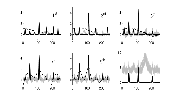
Figure 1: Partial sums of penalized estimates. The first five odd-numbered partial sums from (7) for three penalties: 2nd-derivative (dashed), ridge (gray), targeted PEER (black; see text in sections 2.1 and 7.1). The last panel displays $\beta$ (black) and 15 predictors, $x_{i}$ (gray), from the simulation.

In this toy example, visual structure (spatial location) is used to define a regularization process that easily outperforms uninformed methods of penalization. Less visual examples where the penalty is defined by a set of laboratory-derived structure (in Raman spectroscopy curves) is given in sections 7.2 and 7.3; see Figure 2. In that setting, and in general, the role played by $L$ is appropriately viewed in terms of a preferred subspace in $\mathbb{R}^{p}$ determined by its singular vectors. Algebraic details about how structure in the estimation process is determined jointly by $X$ and $L\neq I$ are described next.

3 Penalized least squares and the GSVD

Of the many methods for estimating a coefficient function discussed in the Introduction, nearly are all aimed at imposing geometric or “functional” structure into the process via the use of basis functions in some manner. An alternative to choosing a basis outright is to exploit the structure imposed by an informed choice of penalty operator. The basis, determined by a pair $(X,L)$, can be tailored toward structure of interest by the choice of $L$. When this is carried out in the least-squares setting of (1), the algebraic properties of the GSVD explicitly reveal how the structure of the estimate is inherited from the spectral properties of $(X,L)$.

3.1 The GSVD

For a given linear penalty $L$ and parameter $\alpha>0$, the estimate in (1) takes the form

$$\tilde{\beta}_{\alpha,L}=(X^{\prime}X+\alpha L^{\prime}L)^{-1}X^{\prime}y.$$ (3)

This cannot be expressed using the singular vectors of $X$ alone, but the generalized singular value decomposition of the pair $(X,L)$ provides a tractable and interpretable series expansion. The GSVD appears in the literature in a variety of forms and notational conventions. Here we provide the necessary notation and properties of the GSVD for our purposes (see, e.g., [19]) but refer to [4, 13, 35] for a complete discussion and details about its computation. See also the comments of Bingham and Larntz [3].

Assume $X$ is an $n\times p$ matrix ($n\leq p$) of rank $n$, $L$ is an $m\times p$ matrix ($m\leq p$) of rank $m$. We also assume that $n\leq m\leq p\leq m+n$, and the rank of the $(n+m)\times p$ matrix $Z:=[X^{\prime}\ L^{\prime}]^{\prime}$ is $p$. A unique solution is guaranteed if the null spaces of $X$ and $L$ intersect trivially: $\mathop{\rm Null}(L)\cap\mathop{\rm Null}(X)=\{0\}$. This is not necessary for implementation, but it is natural in our applications and simplifies the notation. In addition, the condition $p>n$ is not required, but rather than present notation for multiple cases, this will be assumed.

Given $X$ and $L$, the following matrices exist and form the decomposition below: an $n\times n$ matrix $U$ and an $m\times m$ matrix $V$, each with orthonormal columns, $U^{\prime}U=I$, $V^{\prime}V=I$; diagonal matrices $S$ ($n\times n$) and $M$ ($m\times m$); and a nonsingular $p\times p$ matrix $W$ such that

$$X =U\underline{S}W^{-1}\,,\qquad\ \underline{S}=\left[\begin{array}[]{cc}0&S\end{array}\right],\qquad S=\text{diag}\{\sigma_{k}\}$$ (4)

$$L =V\underline{M}W^{-1}\,\qquad\underline{M}=\left[\begin{array}[]{cc}M&0\end{array}\right],\qquad M=\text{diag}\{\mu_{k}\}.$$

Here, $S$ and $M$ are of the form $S=\left[\begin{array}[]{cc}S_{1}&0\\ 0&I_{p-m}\end{array}\right]$ and $M=\left[\begin{array}[]{cc}I_{p-n}&0\\ 0&M_{1}\end{array}\right]$, whose submatrices $S_{1}$ and $M_{1}$ have $q:=n+m-p$ diagonal entries ordered as

$$\begin{aligned} 0&\leq\sigma_{1}\leq\sigma_{2}\leq\cdots\leq\sigma_{q}\leq 1\\ 1&\geq\mu_{1}\geq\mu_{2}\geq\cdots\geq\mu_{q}\geq 0\end{aligned}\qquad\mbox{where}\qquad\sigma_{k}^{2}+\mu_{k}^{2}=1,\quad k=1,...,q,$$ (5)

These matrices satisfy

$$W^{\prime}X^{\prime}XW=\left[\begin{array}[]{ccc}0&0&0\\ 0&S_{1}^{2}&0\\ 0&0&I\end{array}\right]=\underline{S}^{\prime}\underline{S},\qquad W^{\prime}L^{\prime}LW=\left[\begin{array}[]{ccc}I&0&0\\ 0&M_{1}^{2}&0\\ 0&0&0\end{array}\right]=\underline{M}^{\prime}\underline{M},$$ (6)

with $\underline{S}^{\prime}\underline{S}+\underline{M}^{\prime}\underline{M}=I$.

Denote the columns of $U$, $V$ and $W$ by $u_{k}$, $v_{k}$ and $w_{k}$, respectively. In spite of the notation, the generalized singular vectors $u_{k}$ and $v_{k}$ are not the same as the ordinary singular vectors of $X$ in Section 2. They are the same when $L=I$, although their ordering is reversed; in that case, the ordinary singular values correspond to $\gamma_{k}:=\sigma_{k}/\mu_{k}$ for $\mu_{k}>0$. By the convention used for ordering the GS values and vectors, the last few columns of $W$ span the subspace $\mathop{\rm Null}(L)$ (or, if $\mathop{\rm Null}(L)$ is empty, they correspond to the smallest GS values, $\mu_{k}$). We set $d=\dim(\mathop{\rm Null}(L))$ and note that $\mu_{k}=0$ for $k>n-d$.

Now, equation (6) and some algebra gives $(X^{\prime}X+\alpha L^{\prime}L)^{-1}=W(\underline{S}^{\prime}\underline{S}+\alpha\underline{M}^{\prime}\underline{M})^{-1}W^{\prime}$, and so $\tilde{\beta}_{\alpha,L}=W(\underline{S}^{\prime}\underline{S}+\alpha\underline{M}^{\prime}\underline{M})^{-1}\underline{S}^{\prime}U^{\prime}y$. A consequence of the ordering adopted for the GS values and vectors is that the first $p-n$ columns of $W$ play no role in this solution; see equation (4). So we can replace $W$ by the $p\times n$ matrix, $W_{n}$, consisting of the last $n$ columns of $W$ (corresponding to the indices $p-n+1$ to $p$). We index the columns of $W_{n}$ as $w_{1}$,…,$w_{n}$ which is consistent with the indexing established in (5) for the singular values in $S$ and $M$. Therefore, the $L$-penalized estimate can be expressed as a series in terms of GS values as

$$\tilde{\beta}_{\alpha,L}=\sum_{k=1}^{n-d}\left(\frac{\sigma_{k}^{2}}{\sigma_{k}^{2}+\alpha\mu_{k}^{2}}\right)\frac{1}{\sigma}_{k}u_{k}^{\prime}y\,w_{k}\,+\sum_{k=n-d+1}^{n}u_{k}^{\prime}y\,w_{k}.$$ (7)

This GSV expansion corresponds to a new basis for the estimation process: the estimate is expressed in terms of GS vectors $\{w_{k}\}$ determined jointly by $X$ and $L$; cf. the ridge estimate in (2).

For more compact notation used later, define the $(n-d)\times(n-d)$ diagonal matrix $\Gamma=\mathop{\rm diag}\{\gamma_{k}=\sigma_{k}/\mu_{k}\}_{k=1}^{n-d}$. For brevity, set $\mathop{\rm o}:=n-d$ and let $A_{\mathop{\rm o}}$ denote the first $\mathop{\rm o}$ columns of a matrix $A$. Also, denote by $A_{\mathop{\o}}$ the last $d$ columns of $A$. In particular, the range of $W_{\mathop{\o}}$ is $\mathop{\rm Null}(L)$. Using this notation, (7) may be written concisely as

$$\tilde{\beta}_{\alpha,L}=W_{n\mathop{\rm o}}F^{\alpha}\Gamma^{\dagger}{U_{\mathop{\rm o}}}^{\prime}y+W_{\mathop{\o}}{U_{\mathop{\o}}}^{\prime}y,$$ (8)

where $F^{\alpha}=\mathop{\rm diag}\left\{\frac{\sigma_{k}^{2}}{\sigma_{k}^{2}+\alpha\mu_{k}^{2}}\right\}_{k=1}^{n-d}$.

In summary, the utility of a penalty $L$ depends on whether the true coefficient function shares structural properties with this GSVD basis, $\{w_{k}\}_{k=1}^{n}$. With regard to this, the importance of the parameter $\alpha$ may be reduced by a judicious choice of $L$ since the terms in (7) corresponding to the vectors $\{w_{k}:\mu_{k}=0\}$ are independent of the parameter $\alpha$ [53].

As we’ll see, bias enters the estimate to the extent that the vectors $\{w_{k}:\mu_{k}\neq 0\}$ appear in the expansion (7). The portion of $\tilde{\beta}_{\alpha,L}$ that extends beyond the subspace $\mathop{\rm Null}(L)$ is constrained by a sphere (of radius determined by $\alpha$); this portion corresponds to bias. Hence, $L$ may be chosen in such a way that the bias and variance of $\tilde{\beta}_{\alpha,L}$ arises from a specific type of structure, potentially decreasing bias without increasing complexity of the model. As a common example, $L=\mathcal{D}^{2}$ introduces smooth bias structured by low-frequency trigonometric functions.

3.2 Bias and variance and the choice of penalty operator

Begin by observing that the penalized estimate $\tilde{\beta}_{\alpha,L}$ in (3) is a linear transformation of any solution to the normal equations. Indeed, define $X^{\#}\equiv X^{\#}_{\alpha,L}=(X^{\prime}X+\alpha L^{\prime}L)^{-1}X^{\prime}$ and note that if $\hat{\beta}$ denotes any solution to $X^{\prime}X\beta=X^{\prime}y$, then $\tilde{\beta}_{\alpha,L}=X^{\#}X\hat{\beta}+X^{\#}\epsilon$. The resolution operator $X^{\#}X$ reflects the extent to which the estimate in (7) is linearly transformed relative to an exact solution. In particular, $E(\tilde{\beta}_{\alpha,L})=X^{\#}X\hat{\beta}$. Additionally, we have $\mbox{bias}(\tilde{\beta}_{\alpha,L})=(I-X^{\#}X)\beta=\alpha(X^{\prime}X+\alpha L^{\prime}L)^{-1}L^{\prime}L\beta$, and so $||\mbox{bias}(\tilde{\beta}_{\alpha,L})||\leq||\alpha(X^{\prime}X+\alpha L^{\prime}L)^{-1}L^{\prime}||\,||L\beta||$. Hence bias can be controlled by the choice of $L$, with an estimate being unbiased whenever $L\beta=0$. There is a tradeoff, of course, and equation (10) below quantifies the effect on the variance as determined by $W_{\mathop{\o}}$ (i.e., $\{w_{k}\}_{k=n-d+1}^{n}$) if $\mathop{\rm Null}(L)$ is chosen to be too large.

More generally, the decompositions in (4) lead to an expression for the resolution matrix as $X^{\#}X=W(\underline{S}^{\prime}\underline{S}+\alpha\underline{M}^{\prime}\underline{M})^{-1}\underline{S}^{\prime}\underline{S}W^{-1}$, and so $I-X^{\#}X=\alpha W(\underline{S}^{\prime}\underline{S}+\alpha\underline{M}^{\prime}\underline{M})^{-1}\underline{M}^{\prime}\underline{M}W^{-1}$. Again, from equation (4), the first $p-n$ rows of $W^{-1}$ are not used. For notational convenience, define $\tilde{W}:=W^{\prime-1}$ (note, $\tilde{W}$ plays a role analogous to $V\equiv V^{\prime-1}$ in the SVD). As before, let $\tilde{W}_{n}$ denote the $p\times n$ matrix consisting of the last $n$ columns of $\tilde{W}$ and note that in equation (4), $X=U\underline{S}W^{-1}=US(\tilde{W}_{n})^{\prime}$. Hence, $I-X^{\#}X=\alpha W_{n}(S^{2}+\alpha M^{2})^{-1}M^{2}(\tilde{W}_{n})^{\prime}$, and so the bias of $\tilde{\beta}_{\alpha,L}$ can be expressed as

$$\mbox{bias}(\tilde{\beta}_{\alpha,L})=(I-X^{\#}X)\beta=\sum_{k=1}^{n-d}\frac{\alpha\mu_{k}^{2}}{\sigma_{k}^{2}+\alpha\mu_{k}^{2}}w_{k}\tilde{w_{k}}^{\prime}\beta$$ (9)

where $\tilde{w}_{k}$ is the $k$th column of $\tilde{W}$. In particular, the bias vector (9) is contained in $\mathop{\rm span}\{w_{k}:\mu_{k}\neq 0\}$, whereas the estimate $\tilde{\beta}_{\alpha,L}$ is in $\mathop{\rm span}\{w_{k}:\sigma_{k}\neq 0\}$. In the special case that $X^{\prime}X$ is invertible, then $\beta=WS^{-1}U^{\prime}y$ and $\mbox{bias}(\tilde{\beta}_{\alpha,L})=\sum_{k}\left(\frac{\alpha\mu_{k}^{2}}{\sigma_{k}^{2}+\alpha\mu_{k}^{2}}\right)\frac{1}{\sigma_{k}}u_{k}^{\prime}y\,w_{k}$ (see [28]).

A counterpart is an expression for the variance in terms of the GSVD. Let $\Sigma$ denote the covariance for $\epsilon$. Then $\mathop{\rm var}(\tilde{\beta}_{\alpha,L})=\mathop{\rm var}(X^{\#}X\beta+X^{\#}\epsilon)=X^{\#}\Sigma(X^{\#})^{\prime}$. Assuming $\Sigma=\sigma_{\epsilon}I$, this simplifies to

$$\mathop{\rm var}(\tilde{\beta}_{\alpha,L})=\sigma_{\epsilon}^{2}X^{\#}(X^{\#})^{\prime}=\sigma_{\epsilon}^{2}\left(\sum_{k=1}^{n-d}\frac{\sigma_{k}^{2}}{(\sigma_{k}^{2}+\alpha\mu_{k}^{2})^{2}}w_{k}w_{k}^{\prime}+\sum_{k=n-d+1}^{n}w_{k}w_{k}^{\prime}\right).$$ (10)

An interesting perspective of the bias-variance tradeoff is provided by the relationship between the GS-values in (5) and their role in equations (9) and (10). Moreover, these lead to an explicit expression for the mean squared error (MSE) of a PEER estimate. Since $E(\tilde{\beta}_{\alpha,L})=X^{\#}X\beta$,

$$\mbox{MSE}(\tilde{\beta}_{\alpha,L}) =E(||\beta-\tilde{\beta}_{\alpha,L}||^{2})=E(||\beta||^{2}+||\tilde{\beta}_{\alpha,L}||^{2}-2\langle\beta,\tilde{\beta}_{\alpha,L}\rangle)$$ (11)

$$=||\beta-X^{\#}X\beta||^{2}+\sigma_{\epsilon}^{2}\,\mbox{trace}(X^{\#}{X^{\#}}^{\prime})$$

$$=||\mathop{\rm bias}(\tilde{\beta}_{\alpha,L})||^{2}+\sigma_{\epsilon}^{2}\sum_{k=1}^{n-d}\frac{\sigma_{k}^{2}}{(\sigma_{k}^{2}+\alpha\mu_{k}^{2})^{2}}||w_{k}||^{2}.$$

The GS-vectors $\{w_{k}\}$ are not necessarily orthogonal, although they are $X^{\prime}X$-orthogonal; see (6). Consequently, a bound, rather than equality, for the MSE in terms of the GS values/vectors is the best one can do in general:

$$\mbox{MSE}(\tilde{\beta}_{\alpha,L})\leq\left(\sum_{k=1}^{n-d}\frac{\alpha\mu_{k}^{2}}{\sigma_{k}^{2}+\alpha\mu_{k}^{2}}\tilde{w_{k}}^{\prime}\beta\,||w_{k}||\right)^{2}+(\mbox{the second term in \eqref{eq:MSE_beta}}).$$ (12)

As a final remark, recall that one perspective on ridge estimation defines fictitious data from an orthogonal “experiment,” represented by an $L$, and expresses $I$ as $I=L^{\prime}L$ [29]. Regardless of orthogonality this applies to any penalized estimate and $L$ may similarly be viewed as augmenting the data, influencing the estimation process through its eigenstructure; the response, $y$, is set to zero for these supplementary “data”. In this view, equation (3) can be written as $Z\beta=\underline{y}$ where $Z=\left[\begin{array}[]{c}X\\ \sqrt{\alpha}L\end{array}\right]$ and $\underline{y}=\left[\begin{array}[]{c}y\\ 0\end{array}\right]$. This formulation proves useful in section 5.3 when assuring that the estimation process is stable with respect to perturbations in $X$ and the choice of $L$.

4 Structured penalties

A structured penalty refers to a second term in (1) that involves an operator chosen to encourage certain functional properties in the estimate. A prototypical example is a derivative operator which imposes smoothness via its eigenstructure. Here we describe several examples of structured penalties, including two that were motivated heuristically and implemented without regard to the spectral properties that define their performance. Sections 3.2 and 5.3 provide a complete formulation of their properties as revealed by the GSVD.

4.1 The penalty of C. Goutis

The concept of using a penalty operator whose eigenstructure is targeted toward specific properties in the predictors appears implicitly in the work of C. Goutis [14]. This method aimed to account for the “functional nature of the predictors” without oversmoothing and, in essence, considered the inverse of a smoothing penalty. Specifically, if $\Delta$ denotes a discretized second-derivative operator (with some specified boundary conditions), the minimization in (1) was replaced by $\min_{\beta}\{||Y-X\Delta^{\prime}\Delta\beta||_{\mathbb{R}^{n}}^{2}+\alpha||\Delta\beta||_{L^{2}}^{2}\}$. Here, the term $X\Delta^{\prime}\Delta\beta$ can be viewed as the product of $X\Delta^{\prime}$ (derivatives of the predictor curves) and $\Delta\beta$ (derivative of $\beta$). Defining $\gamma:=\Delta^{\prime}\Delta\beta$ and seeking a penalized estimate of $\gamma$ leads to

$$\tilde{\gamma} =(X^{\prime}X+\alpha(\Delta^{\prime}\Delta)^{\dagger})^{-1}X^{\prime}y$$ (13)

$$=\mathop{\rm arg\,min}_{\gamma}\{||y-X\gamma||^{2}+\alpha\langle\gamma,(\Delta^{\prime}\Delta)^{\dagger}\gamma\rangle\}.$$

In [14], the properties of $\tilde{\gamma}$ were conjectured to result from the eigenproperties of $(\Delta^{\prime}\Delta)^{\dagger}$. This was explored by ignoring $X$ and plotting some eigenvectors of $(\Delta^{\prime}\Delta)^{\dagger}$. The properties of this method become transparent, however, when formulated in terms of the GSVD. That is, let $L:=((\Delta^{\prime}\Delta)^{\dagger})^{1/2}$ and note the functions that define $\hat{\gamma}$ are influenced most by the highly oscillatory eigenvectors of $L$ which correspond to its smallest eigenvalues; see equations (5) and (7).

This approach was applied in [14] only for prediction and has drawbacks in producing an interpretable estimate, especially for non-smooth predictor curves. The general insight is valid, however, and modifications of this penalty can be used to produce more stable results. The operator $(\Delta^{\prime}\Delta)^{\dagger}$ essentially reverses the frequency properties of the eigenvectors of $\Delta$ and is an extreme alternative to this smoothing penalty. An eigenanalysis of the pair $(X,L)$, however, suggests penalties that may be more suited to the problem. This is illustrated in Section 7.

4.2 Targeted penalties

Given some knowledge about the relevant structure, a penalty can be defined in terms of a subspace containing this structure. For example, suppose $\beta\in\mathcal{Q}:=\mathop{\rm span}\{q_{j}\}_{j=1}^{d}$ in $L^{2}(I)$. Set $Q=\sum_{j=1}^{d}q_{j}\otimes q_{j}$ and consider the orthogonal projection $P_{\mathcal{Q}}=QQ^{\dagger}$. (Here, $q\otimes q$ denotes the rank-one operator $f\mapsto\langle f,q\rangle q$, for $f\in L^{2}(I)$.) For $L=I-P_{\mathcal{Q}}$, then $\beta\in\mathop{\rm Null}(L)$ and $\tilde{\beta}_{\alpha,L}$ is unbiased. The problem may still be underdetermined so, more pragmatically, define a decomposition-based penalty

$$L\equiv L_{\mathcal{Q}}=a(I-P_{\mathcal{Q}})+bP_{\mathcal{Q}}$$ (14)

for some $a,b\geq 0$. Heuristically, when $a>b>0$ the effect is to move the estimate towards $Q$ by preferentially penalizing components orthogonal to $\mathcal{Q}$; i.e., assign a prior favoring structure contained in the subspace $\mathcal{Q}$. To implement the tradeoff between the two subspaces, we view $a$ and $b$ as inversely related, $ab=$ const. The analytical properties of estimates that arise from this are developed in the next section and illustrated numerically in Section 7. For example, bias is substantially reduced when $\beta\subset\mathcal{Q}$, and equation (19) quantifies the tradeoff with respect to variance when the prior $\mathcal{Q}$ is chosen poorly.

More generally, one may penalize each subspace differently by defining $L=\alpha_{1}(I-P_{\mathcal{Q}})\mathcal{L}_{1}(I-P_{\mathcal{Q}})+\alpha_{2}P_{\mathcal{Q}}\mathcal{L}_{2}P_{\mathcal{Q}}$, for some operators $\mathcal{L}_{1}$ and $\mathcal{L}_{2}$. This idea could be carried further: for any orthogonal decomposition of $L^{2}(I)$ by subspaces $\mathcal{Q}_{1},\dots,\mathcal{Q}_{J}$, let $P_{j}$ be the projection onto $\mathcal{Q}_{j}$. Then the multi-space penalty $L=\sum_{j=1}^{J}\alpha_{j}P_{j}$ leads to the estimate

$$\tilde{\beta}=\mathop{\rm arg\,min}_{\beta}\{||y-X\beta||^{2}+\sum_{j=1}^{J}\alpha_{j}||P_{j}\beta||^{2}\}.$$

This concept was applied in the context of image recovery (where $X$ represents a linear distortion model for a degraded image $y$) by Belge et al. [1].

The examples here illustrate ways in which assumptions about the structure of a coefficient function can be incorporated directly into the estimation process. In general, any estimation of $\beta$ imposes assumptions about its structure (either implicitly or explicitly) and section 3.2 shows that the bias-variance tradeoff involves a choice on the type of bias (spatial structure) as well as the extent of bias (regularization parameter(s)).

5 Some analytical properties

Any direct comparison between estimates using different penalty operators is confounded by the fact there is no simple connection between the generalized singular values/vectors and the ordinary singular values/vectors. Therefore, we first consider the case of targeted or projection-based penalties (14). Within this class, we introduce a parameterized family of estimates that are comprised of ordinary singular values/vectors. Since the ridge and PCR estimates are contained in (or a limit of) this family, a comparison with some targeted PEER estimates is possible. For more general penalized estimates, properties of perturbations provide some less precise relationships; see proposition 5.6.

5.1 Transformation to standard form

We have reason to consider decomposition-based penalties (14) in which $L$ is invertible. In this case, an expression for the estimate does not involve the second term in (8), and decomposing the first term into two parts will be useful. For this, we find it convenient to use the standard-form transformation due to Elden [11] in which the penalty $L$ is absorbed into $X$. This transformation also provides a computational alternative to the GSVD which, for projection-based penalties in particular, can be less computationally expensive; see, e.g., [25]. By this transformation of $X$, a general PEER estimate ($L\neq I$) can be expressed via a ridge-regression process.

Define the $X$-weighted generalized inverse of $L$ and the corresponding transformed $X$ as:

$$L_{X}^{\dagger}:=(I-[X(I-L^{\dagger}L)]^{\dagger}X)L^{\dagger}\quad\mbox{and}\quad\mathbbm{X}:=X\,L_{X}^{\dagger};$$

see [11, 19]. In terms of the GSVD components (4), the transformed $X$ is $\mathbbm{X}=U\Gamma V^{\prime}$. In particular, the diagonal elements of $\Gamma=SM^{\dagger}$ are the ordinary singular values of $\mathbbm{X}$, but in reversed order. Moreover, a PEER estimate can be obtained from a ridge-like penalization process with respect to $\mathbbm{X}$. That is, for

$$\tilde{\mathbb{\bbbeta}}_{\alpha}=\mathop{\rm arg\,min}_{\mathbb{\bbbeta}}\{||\mathbbm{y}-\mathbbm{X}\mathbb{\bbbeta}||^{2}+\alpha||\mathbb{\bbbeta}||^{2}\}\quad\mbox{where}\quad\mathbbm{y}=[X(I-L^{\dagger}L)]^{\dagger}y,$$ (15)

then

$$\tilde{\beta}_{\alpha,L}=L_{X}^{\dagger}\tilde{\mathbb{\bbbeta}}_{\alpha}+\mathbbm{y}.$$

Note that the transformed estimate as given in terms of the GSVD factors is: $\tilde{\bbbeta}_{\alpha}=VF\Gamma^{\dagger}U^{\prime}y$, where $F=\mathop{\rm diag}\{\gamma_{k}^{2}/(\gamma_{k}^{2}+\alpha)\}$.

In what follows we consider invertible $L$ in which case $L_{X}^{\dagger}=L^{-1}$ and $[X(I-L^{\dagger}L)]^{\dagger}=0$. In particular, $\tilde{\beta}_{\alpha,L}=L^{-1}\tilde{\mathbb{\bbbeta}}_{\alpha}$. For the penalty (14) of the form $L=a(I-P_{\mathcal{Q}})+bP_{\mathcal{Q}}$, then $L^{-1}=\frac{1}{a}(I-P_{\mathcal{Q}})+\frac{1}{b}P_{\mathcal{Q}}$, and so $\mathbbm{X}=\frac{1}{a}X(I-P_{\mathcal{Q}})+\frac{1}{b}XP_{\mathcal{Q}}$. The regularization parameter, previously denoted by $\alpha$, can be absorbed into the values $a$ and $b$, so we will denote this PEER estimate $\tilde{\beta}_{\alpha,L}$ simply as $\tilde{\beta}_{a,b}$.

Remark 5.1.

When $a=b=\sqrt{\alpha}$, this is simply a ridge estimate: $\tilde{\beta}_{a,b}=\tilde{\beta}_{\alpha,I}$. Therefore, the best performance among this family of estimates is as least as good as the performance of ridge, regardless of the choice of $\mathcal{Q}$.

5.2 SVD targeted penalties

Consider the special case in which $\mathcal{Q}$ is the span of the $d$ largest right singular vectors of an $n\times p$ matrix $X$ of rank $n$. Let $X=U\left[\begin{array}[]{cc}0&D\end{array}\right]V^{\prime}$ be an ordinary singular value decomposition where $D$ is a diagonal matrix of singular values. For consistency with the GSVD notation, these will be ordered as $0\leq\sigma_{1}\leq\cdots\leq\sigma_{n}$. As before, the first $p-n$ columns of $V$ are not used. Rather than introduce extra notation, we write $X=UDV^{\prime}$, letting $V$ denote the $n\times p$ whose columns correspond to the singular vectors in $D$. So now, the last $d$ columns of $V$ correspond to the $d$ largest singular values of $X$ (i.e., $Q=V_{\mathop{\o}}$).

We are interested interested in the penalty $L=a(I-P_{\mathcal{Q}})+bP_{\mathcal{Q}}$, where $d=\dim(\mathop{\rm Null}(I-P_{\mathcal{Q}}))$. Similar to before, set $\mathop{\rm o}=n-d$ and define $\mathop{\rm o}\times\mathop{\rm o}$ and $d\times d$ submatrices, $D_{\mathop{\rm o}}$ and $D_{\mathop{\o}}$, of $D$ as

$$D=\left[\begin{array}[]{cc}D_{\mathop{\rm o}}&0\\ 0&D_{\mathop{\o}}\end{array}\right];\quad\mbox{also set}\quad\Lambda=\left[\begin{array}[]{cc}aI_{\mathop{\rm o}}&0\\ 0&bI_{d}\end{array}\right].$$ (16)

Here, $P_{\mathcal{Q}}=V_{\mathop{\o}}{V_{\mathop{\o}}}^{\prime}$ and $(I-P_{\mathcal{Q}})=V_{\mathop{\rm o}}{V_{\mathop{\rm o}}}^{\prime}$ and so,

$$\mathbbm{X} =\frac{1}{a}UDV^{\prime}(V_{\mathop{\rm o}}{V_{\mathop{\rm o}}}^{\prime})+\frac{1}{b}UDV^{\prime}(V_{\mathop{\o}}{V_{\mathop{\o}}}^{\prime})=\frac{1}{a}UD\left[\begin{array}[]{c}{V_{\mathop{\rm o}}}^{\prime}\\ 0\end{array}\right]+\frac{1}{b}UD\left[\begin{array}[]{c}0\\ {V_{\mathop{\o}}}^{\prime}\end{array}\right]$$

$$=U\left[\begin{array}[]{c}\frac{1}{a}D_{\mathop{\rm o}}{V_{\mathop{\rm o}}}^{\prime}\\ 0\end{array}\right]+U\left[\begin{array}[]{c}0\\ \frac{1}{b}D_{\mathop{\o}}{V_{\mathop{\o}}}^{\prime}\end{array}\right]=U(D\Lambda^{-1})V^{\prime}$$

This decomposition implies that the ridge estimate in (15) is of the following form: setting $G=D\Lambda^{-1}$, denoting its diagonal entries by $\{\gamma_{k}\}$, and defining $F=\mathop{\rm diag}\{\gamma_{k}^{2}/(\gamma_{k}^{2}+1)\}$ gives $\tilde{\bbbeta}=VFG^{\dagger}U^{\prime}y$. Now,

$$L^{-1}V=\frac{1}{a}V_{\mathop{\rm o}}{V_{\mathop{\rm o}}}^{\prime}V+\frac{1}{b}V_{\mathop{\o}}{V_{\mathop{\o}}}^{\prime}V=\left[\begin{array}[]{c}V_{\mathop{\rm o}}\\ V_{\mathop{\o}}\end{array}\right]\left[\begin{array}[]{cc}\frac{1}{a}I_{\mathop{\rm o}}&0\\ 0&\frac{1}{b}I_{d}\end{array}\right]=V\Lambda^{-1}$$

and so $\tilde{\beta}_{a,b}=L^{-1}\tilde{\bbbeta}=L^{-1}(VFG^{\dagger}U^{\prime}y)=V\Lambda^{-1}F\Lambda D^{-1}U^{\prime}y$. By the decomposition (16),

$$\tilde{\beta}_{a,b}=V_{\mathop{\rm o}}F_{\mathop{\rm o}}D_{\mathop{\rm o}}^{-1}{U_{\mathop{\rm o}}}^{\prime}y+V_{\mathop{\o}}F_{\mathop{\o}}D_{\mathop{\o}}^{-1}{U_{\mathop{\o}}}^{\prime}y.$$

This shows that the estimate decomposes as follows.

Theorem 5.2.

Let $\mathcal{Q}$ be the span of the largest $d$ right singular vectors of $X$. Set $L=a(I-P_{\mathcal{Q}})+bP_{\mathcal{Q}}$. Then, in terms of the notation above, the estimate $\tilde{\beta}_{a,b}$ decomposes as

$$\tilde{\beta}_{a,b}=\sum_{k=1}^{n-d}\left(\frac{\sigma_{k}^{2}}{\sigma_{k}^{2}+a^{2}}\right)\frac{1}{\sigma}_{k}u_{k}^{\prime}y\,v_{k}+\sum_{k=d+1}^{n}\left(\frac{\sigma_{k}^{2}}{\sigma_{k}^{2}+b^{2}}\right)\frac{1}{\sigma}_{k}u_{k}^{\prime}y\,v_{k},$$ (17)

where the left and right terms are independent of $b$ and $a$, respectively.

Similar arguments can be used to decompose an estimate for arbitrary $\mathcal{Q}$:

$$\tilde{\beta}_{a,b}=\sum_{k=1}^{n-d}\left(\frac{\sigma_{k}^{2}}{\sigma_{k}^{2}+a^{2}\mu_{k}^{2}}\right)\frac{1}{\sigma}_{k}u_{k}^{\prime}y\,w_{k}+\sum_{k=d+1}^{n}\left(\frac{\sigma_{k}^{2}}{\sigma_{k}^{2}+b^{2}\mu_{k}^{2}}\right)\frac{1}{\sigma}_{k}u_{k}^{\prime}y\,w_{k}.$$ (18)

In this case, however, all terms are dependent on both $a$ and $b$. Indeed, using notation as in (8) one can decompose $\mathbbm{X}=\frac{1}{a}U\Gamma_{\mathop{\rm o}}V^{\prime}+\frac{1}{b}U\Gamma_{\mathop{\o}}V^{\prime}$ and obtain $\tilde{\bbbeta}=VF\Gamma^{\dagger}U^{\prime}y$. However, $L^{-1}V=WM^{\dagger}$, and the non-orthogonal terms provided by $W$ do not decompose the estimate into terms from the orthogonal sum $\mathcal{Q}\oplus\mathcal{Q}^{\perp}$.

The following corollary, along with Remark 5.1, records the manner in which (17) is a family of penalized estimates, parameterized by $a,b>0$ and $d\in\{1,...,n\}$, that extends some standard estimates.

Corollary 5.3.

Under the conditions in Theorem 5.2,

1. when $a>b>0$,  $\tilde{\beta}_{a,b}$ is a sum of weighted ridge estimates on $\mathcal{Q}$ and $\mathcal{Q}^{\perp}$;

2. when $a>0$ and $b=0$, $\tilde{\beta}_{a,0}$ is given by (8), which is a sum of PCR and ridge estimates on $\mathcal{Q}$ and $\mathcal{Q}^{\perp}$, respectively;

3. for each $d$, the PCR estimate $\tilde{\beta}_{\mbox{\tiny PCR}}^{d}$ is the limit of $\tilde{\beta}_{a,0}$ as $a\to\infty$.

In item 2, this estimate is similar to PCR except that a ridge penalty is placed on the least-dominant singular vectors. Under the assumptions here, $w_{k}\equiv v_{k}$ are the ordinary singular vectors of $X$ and the ordinary singular values appear as $\gamma_{k}=\sigma_{k}/\mu_{k}$, for $\mu_{k}>0$. In the second term of (8), the singular vectors are in the null space of $L$ (since $b=0$), and so $\mu_{k}=0$ and $\sigma_{k}=1$, for $k=n-d+1,...,p$. Regarding item 3, although a PCR estimate is not obtained from equation (3) for any $L$, it is a limit of such estimates.

Other decompositions may be obtained simply by using a permutation, such as $Q=\Pi V$, for some $n\times n$ permutation matrix $\Pi$. Stein’s estimate, $\tilde{\beta}_{\alpha,\mbox{\tiny S}}$, also fits into this framework as follows.

When $X^{\prime}X$ is nonsingular, then $\tilde{\beta}_{\alpha,\mbox{\tiny S}}=(X^{\prime}X+\alpha X^{\prime}X)^{-1}X^{\prime}y$ (see, e.g., the class ‘STEIN’ in [10]), and $X^{\prime}X=VD^{\prime}DV^{\prime}$. Hence this estimate arises from the penalty $L_{\mbox{\tiny S}}=DV^{\prime}$. This is a re-weighted version of $L=a(I-P_{\mathcal{Q}})$ where $d=n$, $Q=V$ and the parameter $a$ is replaced by the matrix $D$. The result is a constant filter factor $F=\mathop{\rm diag}\{1/(1+\alpha)\}$. Using $d<n$ and $Q=V_{d}$ is a natural extension of this idea. More generally, $\mathcal{Q}$ may be enriched with functions that span a wider range of structure potentially relevant to the estimate. This concept is illustrated in Section 7.3 where instead of $V_{d}$, we use a $d$-dimensional set of experimentally-derived “template” spectra supplemented with their derivatives to define $\mathcal{Q}$.

As an aside, we note that in a different approach to regularization one can define a general family of estimates arising from the SVD by way of $\tilde{\beta}_{h,\varphi}=V\Sigma_{h}U^{\prime}y$, where $\Sigma_{h}=\mathop{\rm diag}\{\frac{\sigma_{k}}{h}\varphi(\frac{\sigma_{k}^{2}}{h^{2}})\}$, and $\varphi:\mathbb{R}_{+}\to\mathbb{R}$ is an arbitrary continuous function [33]. A ridge estimate is obtained for $\varphi(t)=1/(1+t)$, and PCR obtained for $\varphi(t)=1/t$ if $t>1$, $\varphi(t)=0$ if $t\leq 1$ (an $L^{2}$-limit of continuous functions). This is similar to item 3 in Corollary 5.3, but the family of estimates $\tilde{\beta}_{h,\varphi}$ is formulated in terms of functional filter factors rather than explicit penalty operators. Related to this is the fact that the optimal (with respect to MSE) estimate using SVD filter factors is, in the case $C=\sigma_{\epsilon}I$, expressed as $\tilde{\beta}_{\mbox{\tiny OH}}=VFD^{\dagger}V^{\prime}y$, where $F=\mathop{\rm diag}\{\sigma_{k}^{2}/(\sigma_{k}^{2}+\sigma_{\epsilon}^{2}(v_{k}^{\prime}\beta)^{-2})\}$; see the “ideal filter” of [34]. In fact, it’s easy to check that this optimal estimate can be obtained as $\tilde{\beta}_{\mbox{\tiny OH}}=\tilde{\beta}_{\alpha,L}$ for some $L\neq I$. Since $\tilde{\beta}_{\mbox{\tiny OH}}$ involves knowledge of $\beta$, it is not directly obtainable but it points to the optimality of a PEER estimate.

5.3 The MSE of some penalized estimates.

Theorem 5.2 is used here to show that $\tilde{\beta}_{a,b}$ can have smaller MSE than the ridge or PCR estimates for a wide range of values of $a$ and/or $b$. The MSE is potentially decreased further when $L$ is defined by a more general $\mathcal{Q}$. In that case, a general statement is difficult to formulate but Proposition 5.6 confirms that any improvement in MSE is robust to perturbations in $L$ (e.g., general $\mathcal{Q}$) and errors in $x$.

An immediate consequence of Theorem 5.2 is that the mean squared error for an estimate in this family (17) decomposes into easily-identifiable terms for the bias and variance:

$$\mbox{MSE}(\tilde{\beta}_{a,b})=\sigma_{\epsilon}^{2} \sum_{k=1}^{n-d}\frac{\sigma_{k}^{2}}{(\sigma_{k}^{2}+a^{2})^{2}}+\sum_{k=1}^{n-d}\left(\frac{a^{2}}{\sigma_{k}^{2}+a^{2}}\right)^{2}(v_{k}^{\prime}\beta)^{2}$$ (19)

$$+\sigma_{\epsilon}^{2}\sum_{k=n-d+1}^{n}\frac{\sigma_{k}^{2}}{(\sigma_{k}^{2}+b^{2})^{2}}+\sum_{k=n-d+1}^{n}\left(\frac{b^{2}}{\sigma_{k}^{2}+b^{2}}\right)^{2}(v_{k}^{\prime}\beta)^{2}.$$

The influence of $b=0$ on the estimate is now clear: when the numerical rank of $X$ is small relative to $d$, the $\sigma_{k}$’s in the third term decrease and the contribution to the variance from this term increases—the estimate fails for the same reason that ordinary least-squares fails. Any nonzero $b$ stabilizes the estimate in the same way that a nonzero $\alpha$ stabilizes a standard ridge estimate; the decomposition (17) merely re-focuses the penalty. This is illustrated in Section 7 (Table 1) and in the Appendix (Table 4). Although there are three parameters to consider, the MSE of $\tilde{\beta}_{a,b}$ is relatively insensitive to $b>0$ for sufficiently large $d$. This could be optimized (similar to efforts to optimize the number of principal components) but here we assume some knowledge regarding $\mathcal{Q}$, hence $d$. Relationships between ridge, PCR and PEER estimates in this family $\{\tilde{\beta}_{a,b}\}_{a,b>0}$ can be quantified more specifically as follows.

Proposition 5.4.

Suppose $\beta\in\mathcal{Q}$ and fix $\alpha>0$. Then for any $a>\sqrt{\alpha}$, the ridge estimate satisfies

$$\mbox{MSE}(\tilde{\beta}_{\alpha,I})\equiv\mbox{MSE}(\tilde{\beta}_{\sqrt{\alpha},\sqrt{\alpha}})>\mbox{MSE}(\tilde{\beta}_{a,\sqrt{\alpha}}).$$

Proof.

This follows from the fact that ${V_{\mathop{\rm o}}}^{\prime}\beta=0$ and so the second term in (19) is zero. Therefore, the contribution to the MSE by the first term is decreased whenever $a>\sqrt{\alpha}$. ∎

If $\beta$ is exactly a sum of the $d$ dominant right singular vectors, A PCR estimate using $d$ terms may perform well, but is not optimal:

Proposition 5.5.

If $\beta\in\mathcal{Q}$, a sufficient condition for the PCR estimate to satisfy

$$\mbox{MSE}({\tilde{\beta}^{d}}_{\mbox{\tiny PCR}})\equiv\mbox{MSE}(\tilde{\beta}_{\infty,0})>\mbox{MSE}(\tilde{\beta}_{\infty,b})$$

is

$$\sigma_{\epsilon}^{2}\left(\sum_{k=n-d+1}^{n}\frac{1}{\sigma_{k}^{2}}+\frac{2d}{b^{2}}\right)>||{V_{\mathop{\o}}}^{\prime}\beta||^{2}$$ (20)

Note that the left side of (20) increases without bound as $\sigma_{k}\to 0$. Since $||{V_{\mathop{\o}}}^{\prime}\beta||^{2}=\sum_{k=n-d+1}^{n}(v_{k}^{\prime}\beta)^{2}$, and since the premise of PCR is that $v_{k}^{\prime}\beta$ decreases with decreasing $\sigma_{k}$, this sufficient condition is entirely plausible.

Proof.

The MSE of ${\tilde{\beta}^{d}}_{\mbox{\tiny PCR}}$ consists of the second and third terms of (19):

$$\mbox{MSE}({\tilde{\beta}^{d}}_{\mbox{\tiny PCR}})=\sum_{k=1}^{n-d}(v_{k}^{\prime}\beta)^{2}+\sigma_{\epsilon}^{2}\sum_{k=n-d+1}^{n}\frac{1}{\sigma_{k}^{2}}.$$

In particular, a sufficient condition for this to exceed $\mbox{MSE}(\tilde{\beta}_{\infty,b})$ is for the variance term to exceed the third and fourth terms of (19):

$$\sigma_{\epsilon}^{2}\sum_{k=n-d+1}^{n}\frac{1}{\sigma_{k}^{2}}>\sigma_{\epsilon}^{2}\sum_{k=n-d+1}^{n}\frac{\sigma_{k}^{2}}{(\sigma_{k}^{2}+b^{2})^{2}}+\sum_{k=n-d+1}^{n}\left(\frac{b^{2}}{\sigma_{k}^{2}+b^{2}}\right)^{2}(v_{k}^{\prime}\beta)^{2}.$$

Its easy to check that this is satisfied when (20) holds. ∎

A comment by Bingham and Larntz [3] on the intensive simulation study of ridge regression in [10] notes that “it is not at all clear that ridge methods offer a clear-cut improvement over [ordinary] least squares except for particular orientations of $\beta$ relative to the eigenvectors of $X^{\prime}X$.” Equation (19) repeats this observation relating these two classical methods as well as the minor extensions contained in (17). If, on the other hand, “the orientation of $\beta$ relative to the [$v_{k}$’s]” is not favorable, i.e., if $\beta$ is nowhere near the range of $V$, then a PEER estimate as in (18) is more desirable than (17) (assuming sufficient prior knowledge).

In summary, the family of estimates $\{\tilde{\beta}_{a,b}\}_{a,b>0}$ in (17) represents a hybrid of ridge and PCR estimation. This family—based on the ordinary singular vectors of $X$—is introduced here to provide a framework within which these two familiar estimates can be compared to (slightly) more general PEER estimates. Direct analytical comparison between general PEER estimates is more difficult since there’s no simple relationship between the generalized singular vectors for two different $L$ (including $L=I$ versus $L\neq I$). However, it is important that the estimation process be stable with respect to changes in $L$ and/or $X$. I.e., in going from an estimate in (17) to one in (18), the performance of the estimate should be predictably altered. Given an estimate in Proposition 5.4, if $\mathcal{Q}$ is modified and/or $X$ is observed with error, the MSE of the corresponding estimate, $\tilde{\beta}^{E}_{\alpha,L}$, should be controlled: for sufficiently small perturbation $E$, the corresponding estimate $\mbox{MSE}(\tilde{\beta}^{E}_{\alpha,L})$ should be close to $\mbox{MSE}(\tilde{\beta}_{\alpha,I})$. This “stability” is true in general. To see this, recall $Z=\left[\begin{array}[]{cc}X^{\prime}&\sqrt{\alpha}L^{\prime}\end{array}\right]^{\prime}$ (of rank $p$) and $\underline{y}=\left[\begin{array}[]{cc}y^{\prime}&0\end{array}\right]^{\prime}$. Then another way to represent the estimate (3) is $\tilde{\beta}_{\alpha,L}=Z^{\dagger}\underline{y}$. Let $E=\left[\begin{array}[]{cc}{E_{1}}^{\prime}&{E_{2}}^{\prime}\end{array}\right]^{\prime}$ for some $n\times p$ and $m\times p$ matrices $E_{1}$ and $E_{2}$. Set $Z_{E}=Z+E$ and denote the perturbed estimate by $\tilde{\beta}^{E}_{\alpha,L}=Z_{E}^{\dagger}\underline{y}$. By continuity of the generalized inverse (e.g., [4], Section 1.4), $\lim_{||E||\to 0}Z_{E}^{\dagger}=Z^{\dagger}$ if and only if $\lim_{||E||\to 0}\mathop{\rm rank}(Z_{E})=\mathop{\rm rank}(Z)$. Therefore, provided the rank of $Z$ is not changed by $E$,

$$\lim_{||E||\to 0}||\tilde{\beta}_{\alpha,L}-{\tilde{\beta}^{E}}_{\alpha,L}||\leq\lim_{||E||\to 0}||Z^{\dagger}-Z_{E}^{\dagger}||\,||y||=0,$$

and hence $\mbox{MSE}({\tilde{\beta}^{E}}_{\alpha,L})\to\mbox{MSE}({\tilde{\beta}}_{\alpha,L})$ as $||E||\to 0$. A more specific bound on the difference of estimates can be obtained under the condition $||Z^{\dagger}||||E||<1$ which implies that $||Z_{E}^{\dagger}||<\frac{||Z^{\dagger}||}{1-||Z^{\dagger}||||E||}$. This can be used to obtain the following bound.

Proposition 5.6.

Assume $||Z^{\dagger}||||E||<1$ and let $r=\underline{y}-Z\tilde{\beta}_{\alpha,L}$. Then

$$||\tilde{\beta}_{\alpha,L}-{\tilde{\beta}^{E}}_{\alpha,L}||\leq\frac{||Z^{\dagger}||||E||}{1-||Z^{\dagger}||||E||}\left(||\tilde{\beta}_{\alpha,L}||+||Z^{\dagger}||||r||\right).$$

See [4] and [18].

6 Tuning parameter selection

Despite our focus on the GSVD, the computation of a PEER estimate in (1) does not, of course, require that this decomposition be computed. Rather, the role of the GSVD has been to provide analytical insight into the role a penalty operator plays in the estimation process. For computation, on the other hand, we have chosen to use a method in which the tuning parameter, $\alpha$, is estimated as part of the coefficient-function estimation process.

Because the choice of tuning parameter is so important, many selection criteria have been proposed, including generalized cross-validation (GCV) [9], AIC and its finite sample corrections [55]. As an alternative to GCV and AIC, a recently-proven equivalence between the penalized least squares estimation and a linear mixed model (LMM) representation [6] can be used. In particular, the best linear unbiased predictor (BLUP) of the response $y$ is composed of the best linear unbiased estimator of the fixed effects and BLUP of the random effects for the given values of the random component variances (see [47] and [6]). Within the LMM framework, restricted maximum likelihood (REML) can be used to estimate the variance components and thus the choice of the tuning parameter, $\alpha$, which is equal to the ratio of the error variance and the random effects variance [42]. REML-based estimation of the tuning parameter has been shown to perform at least as well as the other criteria and, under certain conditions, it seen to be less variable than GCV-based estimation [41]. In our case, the penalized least-squares criterion (1) is equivalent to

$$\tilde{\beta}_{\alpha,L}=\mathop{\rm arg\,min}_{\beta}\{||y-X_{unp}\beta_{unp}-X_{pen}\beta_{pen}||^{2}+\alpha||L\beta||^{2}\}$$ (21)

where $\beta=[\beta_{unp}^{\prime}\ \beta_{pen}^{\prime}]^{\prime}$, the $X_{unp}$ corresponds to the unpenalized part of the design matrix, and $X_{pen}$ to the penalized part.

For simplicity of presentation, we describe the transformation with an invertible $L$. However, a generalized inverse can be used in case $L$ is not of full rank; see equation (15). Also, to facilitate a straightforward use of existing linear mixed model routines in widely available software packages (e.g., R [37] or SAS software [43]), we transform the coefficient vector $\beta$ using the inverse of the matrix $L$. Let $X^{\star}=XL$ and $\beta^{\star}=L^{-1}\beta$. Then equation (21) can be modified as follows

$$\tilde{\beta}_{\alpha,L}^{\star}=\mathop{\rm arg\,min}_{\beta}\{||y-X^{\star}\beta^{\star}||^{2}+\alpha||\beta^{\star}||^{2}\}.$$

This REML-based estimation of tuning parameters is used in the application of Section 7.3.

For estimation of the parameters $a$, $b$ and $\alpha$ involved in the decomposition-based penalty of equation (17), we view $a$ and $b$ as weights in a tradeoff between the subspaces and assume $ab=$ const. For implementation, we fix one, estimate the other using a grid search, and use REML to estimate $\alpha$.

7 Numerical examples

To illustrate algebraic properties given in Section 5, we consider PEER estimation alongside some familiar methods in several numerical examples. Section 7.1 elaborates on the simple example in Section 2.1. These mass spectrometry-like predictors are mathematically synthesized in a manner similar to the study of Reiss and Ogden [40] (see also a numerical study in [48]). Here, $\beta$ is also synthesized to represent a spectrum, or specific set of bumps. In contrast, Section 7.3 presents a real application to Raman spectroscopy data in which a set of spectra $\{x_{i}\}$ and nanoparticle concentrations $\{y_{i}\}$ are obtained from sets of laboratory mixtures. This laboratory-based application is preceded in section 7.2 by a simulation that uses these same Raman spectra. In both Raman examples, targeted penalties (14) are defined using discretized functions $q_{j}$ chosen to span specific subspaces, $\mathcal{Q}=\mathop{\rm span}\{q_{j}\}_{j=1}^{d}$. As before, let $Q=\mathop{\rm col}[q_{1},...,q_{d}]$ and $P_{\mathcal{Q}}=QQ^{\dagger}$.

Each section displays the results from several methods, including derivative-based penalties. Implementing these requires a choice of discretization scheme and boundary conditions which define the operator. We use $\mathcal{D}^{2}$ where $\mathcal{D}=[d_{i,j}]$ is a square matrix with entries $d_{i,i}=1$, $d_{i,i+1}=-1$ and $d_{i,j}=0$ otherwise. In addition to some standard estimates, sections 7.3 and 7.2 also consider $\mbox{FPCR}_{R}$, a functional PCR estimate described in [40]. This approach extends the penalized B-spline estimates of [8] and assumes $\beta=B\eta$ where $B$ is an $p\times K$ matrix whose columns consist of $K$ B-spline functions and $\eta$ is a vector of B-spline coefficients. The estimation process takes place in the coefficient space using the penalty $L=\mathcal{D}^{2}$ applied to $\eta$. The $\mbox{FPCR}_{R}$ estimate further assumes $\beta=BV_{d}\,\eta$ ($V_{d}$ as defined in section 2).

Estimation error is defined as mean squared error (MSE) $||\beta-\tilde{\beta}_{\alpha,L}||^{2}$, and the prediction error defined similarly as $\sum_{i}|y_{i}-\tilde{y_{i}}|^{2}$, where $\tilde{y_{i}}=\langle x_{i},\tilde{\beta}\rangle$. Each simulation incorporates response random errors, $\epsilon_{i}\sim N(0,\sigma_{\epsilon}^{2})$, added to the $i$th true response, $y^{\mbox{\tiny true}}_{i}=\langle x_{i},\beta\rangle$. Letting $S_{Y}^{2}$ denote the sample variance in the set $\{y^{\mbox{\tiny true}}_{i}\}_{i=1}^{n}$, the response random errors, $\epsilon_{i}$, are chosen such that $R^{2}:=S_{Y}^{2}/[S_{Y}^{2}+\sigma^{2}_{\epsilon}]$ (the squared multiple correlation coefficient of the true model) takes values 0.6 and 0.8. In sections 7.1 and 7.2, tuning parameters are chosen by a grid search. In section 7.3, tuning parameters are chosen using REML, as described in section 6.

7.1 Bumps Simulation

Here we elaborate on the simple example of section 2.1. This simulation involves bumpy predictor curves $x_{i}(t)$ with a response $y_{i}$ that depends on the amplitudes $x_{i}(t)$ at some of the bump locations, $t=c_{k}$, via the regression function $\beta$. In particular,

$$x_{i}(t)=\sum_{j\in J_{X}}a_{ij}\exp[-b_{j}(t-c_{j})]+e_{i}(t),\quad\beta(t)=\sum_{j\in J_{\beta}}a_{j}\exp[-b_{j}(t-c_{j})],\ \ t\in[0,1]$$

where $J_{X}=\{2,6,10,14,20,26,30\}$, $J_{\beta}=\{6,14,26\}$, $a_{\star}$ are the magnitudes, $b_{\star}$ are the spreads, and $c_{\star}$ are the locations of the bumps. In the first simulation, we set $b_{j}=10000$ and $c_{j}=0.004(8j-1)$, the same for each curve $x_{i}$. This mimics, for instance, curves seen in mass spectrometry data. The assumption $J_{\beta}\subset J_{X}$ simulates a setting in which the response is associated with a subset of metabolite or protein features in a collection of spectra. The $a_{ij}$’s are from a uniform distribution, and $a_{j}=3,5,2$ for $j=6,14,24$, respectively. We consider discretized curves, $x_{i}(t)$, evaluated at $p=250$ points, $t_{j}$, $j=1,\ldots,p$. The sample size is fixed at $n=50$ in each case.

Penalties. We consider a variety of estimation procedures: ridge ($L=I$), second-derivative ($\mathcal{D}^{2}$), a more general derivative operator ($\mathcal{D}^{2}+a\,I$) and PCR. We also define two decomposition-based penalties (14) formed by specific subspaces $\mathcal{Q}=\mathop{\rm span}\{q_{j}\}_{j\in J}$ for $q_{j}$ of the form $q_{j}(t)=a_{j}\exp[b_{j}(t-c_{j})]$, with $c_{j}$ at all locations seen in the predictors, $J_{V}=\{2,6,10,14,20,26,30\}$, or at uniformly-spaced locations, $J_{U}=\{2,4,\ldots,30\}$; denote these penalties by $L_{V}$ and $L_{U}$, respectively.

Simulation results. The simulation incorporates two sources of noise: (i) response random errors, $\epsilon_{i}\sim N(0,\sigma_{\epsilon}^{2})$, added to the $i$th true response so that $R^{2}=0.6,0.8$; (ii) measurement error, $e_{i}\sim N_{p}(0,\sigma_{e}^{2}I)$, added to the $i$th predictor, $x_{i}$. To define a signal-to-noise ratio, $S/N$, set $S_{i}^{2}:=||x_{i}-\mu_{i}||^{2}/(p-1)$, where $\mu_{i}$ is the mean value of $x_{i}$, and set $S_{X}^{2}:=1/n\sum_{i}S_{i}^{2}$. The $e_{i}$ are chosen so that $S/N:=S_{X}/\sigma_{e}=2,5,10$.

Figure 1 shows a few partial sums of (7) for estimates arising from three penalties: $\mathcal{D}^{2}$, $L=I$ and $L_{V}$, when $R^{2}=0.8$ and $S/N=2$. Table 1 gives a summary of estimation errors. The penalty $L_{V}$, exploiting known structure, performs well in terms of estimation error. Not surprisingly, a penalty that encourages low-frequency singular vectors, $\mathcal{D}^{2}$, is a poor choice although $\mathcal{D}^{2}+a\,I$ easily improves on $\mathcal{D}^{2}$ since the GSVs are more compatible with the relevant structure. PCR performs well with estimation errors that can be several times smaller than those of ridge. The number of terms used in PCR ranges here from 8 ($S/N=10$) to 25 ($S/N=2$).

Table 1: Estimation errors (MSE) for simulation with selected bump locations. Sample size is $n=50$.

$R^{2}$	$S/N$	$L_{V}$	$L_{U}$	PCR	ridge	$\mathcal{D}^{2}$	$\mathcal{D}^{2}+a\,I$
0.8	10	4.00	13.81	9.38	34.39	359.83	76.31
0.8	5	3.72	15.46	21.50	40.02	246.17	72.64
0.8	2	4.40	12.96	57.89	58.22	126.75	59.35
0.6	10	9.60	21.60	14.10	50.50	497.70	113.60
0.6	5	10.22	21.65	26.02	50.68	338.70	87.58
0.6	2	11.75	23.18	63.50	67.94	181.75	78.45

Predictably, PCR performance degrades with decreasing $S/N$, a property that is less pronounced, or not shared, by other estimates. Performances of $L_{V}$ and $L_{U}$ illustrate properties described in Section 5.3. As $S/N\to 0$, the ordinary singular vectors of $X$ (on which ridge and PCR rely) decreasingly represent the structure in $\beta$. The GS vectors of $(X,L_{V})$ and $(X,L_{U})$, however, retain structure relevant for representing $\beta$.

Table 2: Prediction errors for simulation with selected bump locations. Sample size is $n=50$. Errors are multiplied by 1000 for display.

$R^{2}$	$S/N$	$L_{V}$	$L_{U}$	PCR	ridge	$\mathcal{D}^{2}$	$\mathcal{D}^{2}+a\,I$
0.8	10	9.0	10.5	10.8	16.6	19.3	12.9
0.8	5	8.4	11.0	12.2	26.7	27.9	17.8
0.8	2	12.9	19.0	53.2	55.7	50.3	40.1
0.6	10	21.4	23.0	23.9	33.0	39.0	26.2
0.6	5	23.9	25.0	29.5	49.2	54.6	34.4
0.6	2	34.4	42.5	90.4	110.4	104.4	77.9

Table 2 summarizes prediction errors. When $S/N$ is large, performance of PCR is comparable with $L_{V}$ and $L_{U}$, but degrades for low $S/N$. Here, even $\mathcal{D}^{2}+a\,I$ provides smaller prediction errors, in most cases, than ridge, $\mathcal{D}^{2}$ or PCR. This illustrates the GS vectors role in (13) and reiterates observations in [14].

7.2 Raman simulation

We consider Raman spectroscopy curves which represent a vibrational response of laser-excited co-organic/inorganic nanoparticles (COINs). Each COIN has a unique signature spectrum and serves as a sensitive nanotag for immunoassays; see [27, 44]. Each spectrum consists of absorbance values measured at $p=600$ wavenumbers. By the Beer-Lambert law, light absorbance increases linearly with a COIN’s concentration and so a spectrum from a mixture of COINs is reasonably modeled by a linear combination of pure COIN spectra. The data here come from experiments that were designed to establish the ability of these COINs to measure the existence and abundance of antigens in single-cell assays.

Let $P_{1},...,P_{10}$ denote spectra from nine pure COINs and one “blank” (no biochemical material), each normalized to norm one. We form in-silico mixtures as follows: $x_{i}=\sum_{k=1}^{10}c_{i,k}P_{k}$, $i=1,...,n$, with coefficients $\{c_{i,k}\}$ generated from a uniform distribution. Figure 2 shows representative spectra from all nine COINs superimposed on a collection of mixture spectra, $\{x_{i}\}_{i=1}^{50}$. Included in Figure 2 is the $\beta$ (dashed curve) used to defined the simulation: $y_{i}=\langle x_{i},\beta\rangle+\epsilon$, $\epsilon\thicksim N(0,\sigma^{2})$.

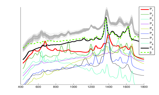
Figure 2: Nine pure COIN spectra, $P_{1},...,P_{9}$, and a coefficient function, $\beta$ (each shifted for display). $\beta$ arises as a solution to the fLM in which $y$ denotes concentrations of $P_{9}$ in an in silico mixture of $50$ COIN spectra, $x_{i}$ (light gray). This $\beta$ is used in the simulation study of Section 7.2.

In this simulation, we have created a coefficient function which, instead of being modeled mathematically, is a curve that exhibits structure of the type found in Raman spectra. Details on the construction of this $\beta$ are in Appendix 9.1 so here we simply note that it arises as a ridge estimate from a set of in-silico mixtures of Raman spectra in which one COIN, $P_{9}$, is varied prominently relative to the others. See Figure 2. Motivation for defining $\beta$ in this way is based on a view that it seems implausible for us to predict the structure of realistic signal in these data and recreate it using polynomials, Gaussians or other analytic functions.

Regardless of its construction, $\beta$ defines signal that allows us to compute estimation and prediction error. The performances of five methods are summarized in Table 3. Note that although $\beta$ was constructed as a ridge estimate (using a different set of in-silico mixtures; see Appendix 9.1), the ridge penalty is not necessarily optimal for recovering $\beta$. This is because the strictly empirical eigenvectors associated with the new spectra may contain structure not informative regarding $y$. Also, in these data, the performance of FPCR_R is adversely affected by a tendency for the estimate to be smooth; cf., Figure 3. The PEER penalty used here is defined by a decomposition-based operator (17) in which $\mathcal{Q}$ is spanned by a 10-dimensional set of pure-COIN spectra (including a blank). The success of such an estimate obviously depends on an informed formation of $\mathcal{Q}$, but as long as the parameter-selection procedure allows for $a=b$, then the set of possible estimates includes ridge as well as estimates with potentially lower MSE than ridge; see Proposition 5.4.

Table 3: Estimation (MSE) and prediction (PE) errors of several penalization methods for the simulation described in Figure 2. Numbers represent the average error from 100 runs. PE errors are multiplied by 1000 for display.

	$L_{Q}$	PCR	ridge	$\mathcal{D}^{2}+a\,I$	FPCRR
MSE	8.91	12.34	13.87	41.69	15.29
PE	0.0071	0.0179	0.0139	0.0131	0.0175

We note that this simulation may be viewed as inherently unfair since the PEER estimate uses knowledge about the relevant structure. However, this is a point worth reemphasizing: when prior knowledge about the structure of the data is available, it can be incorporated naturally into the regression problem.

7.3 Raman Application

We now consider spectra representing true antibody-conjugated COINs from nine laboratory mixtures. These mixtures contain various concentrations of eight COINs (of the nine shown in Figure 2). Spectra from four technical replicates in each mixture are included to create a set of $n=36$ spectra $\{x_{i}\}_{i=1}^{n}$. We designate $P_{1}$ as the COIN whose concentration within each mixture defines $y$. Assuming a linear relationship between the spectra, $\{x_{i}\}$, and the $P_{1}$-concentrations, $\{y_{i}\}$, we estimate $P_{1}$. More precisely, we estimate the structure in $P_{1}$ that correlates most with its concentrations, as manifest in this set of mixtures. The fLM is a simplistic model of this relationship between the concentration of $P_{1}$ and its functional structure, but the physics of this technology imply it is a reasonable starting point.

We present the results of three estimation methods: ridge, FPCR_R and PEER. In constructing a PEER penalty, we note that the informative structure in Raman spectra is not that of low-frequency or other easily modeled features, but it may be obtainable experimentally. Therefore, we define $L$ as in (14) in which $\mathcal{Q}$ contains the span of COIN template spectra: $\mathcal{Q}_{1}=\mathop{\rm span}\{P_{k}\}_{k=1}^{8}$. However, since a single set of templates may not faithfully represent signal in subsequent experiments (with new measurement errors, background and baseline noise etc), we enlarge $\mathcal{Q}$ by adding additional structure related to these templates. For this, set $\mathcal{Q}_{2}=\mathop{\rm span}\{P^{\prime}_{k},P^{\prime\prime}_{k}\}_{k=1}^{8}$, where $P^{\prime}_{k}$ denotes the derivative of spectrum $P_{k}$. (Note, to form $\mathcal{Q}_{2}$, scale-based approximations to these derivatives are used since raw differencing of non-smooth spectra introduces noise.) Then set $\mathcal{Q}=\mathop{\rm span}\{\mathcal{Q}_{1}\cup\mathcal{Q}_{2}\}$ and define $L=a(I-P_{\mathcal{Q}})+bP_{\mathcal{Q}}$.

The regularization parameters in the PEER and ridge estimation processes were chosen using REML, as described in Section 6. For the FPCR_R estimate, we used the R-package refund [39] as implemented in [40].

Since $\beta$ is not known (the model $y=X\beta+\epsilon$ is only approximate), we cannot report MSEs for these three methods. However, the structure of $P_{1}$ is qualitatively known and by experimental design, $y$ is directly associated with $P_{1}$. The goal here is that of extracting structure of the constituent spectral components as manifest in a linear model. This application is similar to the classic problem of multivariate calibration [5, 31] which essentially leads to a regression model using an experimentally-designed set of spectra from laboratory mixes.

The structure in the estimate here is expected to reflect the structure in $P_{1}$ that is correlated with $P_{1}$’s concentrations, $y$. The estimate is not, however, expected to precisely reconstruct $P_{1}$ since $P_{1}$ shares structure with the other COIN spectra not associated with $y$. See Figure 2 where $P_{1}$ is plotted alongside the other COIN spectra. Now, Figure 3 shows plots of the PEER, FPCR_R and ridge estimates of the fLM coefficient function. The PEER estimate, $\tilde{\beta}_{Q}$, provides an interpretable compromise between ridge, which involves no smoothing, and FPCR_R, which appears to oversmooth. For reference, the $P_{1}$ spectrum is also plotted along with a mean-adjusted version of $\tilde{\beta}_{Q}$, $\tilde{\beta}_{Q}+\mu$ (dashed line), where $\mu(t)=(1/36)\sum_{i}x_{i}(t)$, $t\in[400,1800]$.

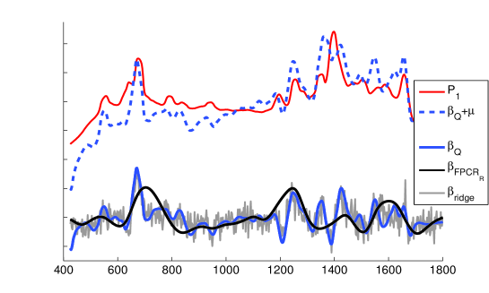
Figure 3: Three estimates for a coefficient function that relates concentrations of $P_{1}$ to its signal in 8-COIN laboratory mixtures. Estimates shown: ridge ($\tilde{\beta}_{\mbox{ridge}}$), FPCR_R ($\tilde{\beta}_{F}$) and PEER ($\tilde{\beta}_{Q}$). For perspective, $P_{1}$ is plotted (in red) and the mean-adjusted PEER estimate, $\tilde{\beta}_{Q}+\mu$ (dashed blue); $\mu$ is the mean of the mixture spectra $\{x_{i}\}_{i=1}^{36}$ (not shown).

Finally, we consider prediction for these methods by forming a new set of spectra from different mixture compositions (different concentrations of each COIN) and, additionally, taken from different batches. This “test” set consists of spectra from four technical replicates in each of 15 mixtures forming a set of $n=60$ spectra, $\{x_{i}^{\mbox{\footnotesize test}}\}_{i=1}^{n}$. As before, $P_{1}$ is the COIN whose concentration within each mixture defines the values $\{y_{i}^{\mbox{\footnotesize test}}\}_{i=1}^{n}$. For the estimates from each of the three methods (shown in Figure 3) we compute the prediction error: $(1/n)\sum_{i}(y_{i}^{\mbox{\footnotesize test}}-\langle x_{i}^{\mbox{\footnotesize test}},\tilde{\beta}\rangle)^{2}$. The errors for PEER, ridge, and FPCR_R estimates are 0.770, 0.752, 2.139, respectively. The ridge estimate here illustrates how low prediction error is not necessarily accompanied by interpretable structure in the estimate (or low MSE) [7].

8 Discussion

As high-dimensional regression problems become more common, methods that exploit a priori information are increasingly popular. In this regard, many approaches to penalized regression are now founded on the idea of “structured” penalties which impose constraints based on prior knowledge about the problem’s scientific setting. There are many ways in which such constraints may be imposed, and we have focused on the algebraic aspects of a penalization process that imposes spatial structure directly into a regularized estimation. This approach fits into the classic framework of $L^{2}$-penalized regression but with an emphasis on the algebraic role that a penalty operator plays to impart structure on the estimate.

The interplay between a structured regularization term and the coefficient-function estimate may not be well understood in part because it is not typically viewed in terms of the generalized singular vectors/values, which is fundamental to this investigation. In particular, any penalized estimate of the form (1) with $L\neq I$ is intrinsically based on GSVD factors in the same way that many common regression methods (such as PCR, ridge, James-Stein, or partial least squares) are intrinsically based on SVD factors. Just as the basics of the ubiquitous SVD are important to understanding these methods, we have aspired to established the basics of the GSVD as it applies to a this general penalized regression setting and to illustrate how the theory underlying this approach can be used inform the choice of penalty operator.

Toward this goal the presentation emphasizes the transparency provided by the partially-empirical eigenvector expansion (7). Properties of the estimate’s variance and bias are determined explicitly by the generalized singular vectors whose structure is determined by the penalty operator. We have restricted attention to additive constraints defined by penalty operators on $L^{2}$ in order to retain the direct algebraic connection between the eigenproperties of the operator pair $(X,L)$ and the spatial structure of $\tilde{\beta}_{\alpha,L}$. Intuitively, the structure of the penalty’s least-dominant singular vectors should be commensurate with the informative structure of $\beta$. The actual effect a penalty has on the properties of the estimate can be quantified in terms of the GSVD vectors/values.

This perspective differs from popular two-stage signal regression methods in which estimation is either preceded by fitting the predictors to a set of (external) basis functions or is followed by a step that smooths the estimate [8, 21, 30, 38, 40]. Instead, structure (smoothness or otherwise) is imposed directly into the estimation process. The implementation of a penalty that incorporates structure less generic than smoothness (or sparseness) requires some qualitative knowledge about spatial structure that is informative. Clearly this is not possible in all situations, but our presentation has focused on how a functional linear model may provide a rigorous and analytically tractable way to take advantage of such knowledge when it exists.

Acknowledgements: The authors wish to thank the referees and associate editor for all of their questions and helpful suggestions which greatly improved the presentation. We also gratefully acknowledge the patience, insight and assistance from Dr. C. Schachaf who provided the Raman spectroscopy data for the examples in Sections 7.2 and 7.3. Research support was provided by the National Institutes of Health grants R01-CA126205, P01-CA053996 and U01-CA086368.

9 Appendix

9.1 Defining $\beta$ for the simulation in section 7.2

This simulation is motivated by an interest in constructing a plausibly realistic $\beta$ whose structure is naturally derived by the scientific setting involving Raman signatures of nanoparticles. Although one could model a $\beta$ mathematically using, say, polynomials or Gaussian bumps (cf., Appendix A.2), such a simulation would be detached from the physical nature of this problem. Instead, we construct a coefficient function that genuinely comes from a functional linear model with Raman spectra as predictors.

We first generate in-silico mixtures of COIN spectra as $x^{o}_{i}=\sum_{k=1}^{9}c_{i,k}P_{k}$, $i=1,...,50$, where $c_{i,k}\sim\mbox{unif}[0,1]$. Designating $P_{9}$ as the COIN of interest, we define response values that correspond to the “concentration” of $P_{9}$ by setting $y^{o}_{i}:=3\,c_{i,9}$, $i=1,...,n$. The factor of 3 imposes a strong association between $P_{9}$ and the response.

Now, the example in section 7.2 aims to estimate a coefficient function that truly comes from a solution to a linear model. However, the equation $y^{o}=X^{o}\beta$ has infinitely many solutions (where $X^{o}$ is the matrix whose $i$th row is $x^{o}_{i}$), so we must we must regularize the problem to obtain a specific $\beta$. For this, we simply use a ridge penalty and designate the resulting solution to be $\beta$. This is shown by the dotted curve in Figure 2 and is qualitatively similar to $P_{9}$.

We note that the simulation in section 7.2 uses the same set of COINs, but a new set of in-silico mixture spectra (i.e., a new set of $\{c_{i,k}\}\sim\mbox{Unif}[0,1]$). In addition, a small amount of measurement error was added, as in section 7.1, to each spectrum during the simulation.

9.2 Frequency domain simulation

We display results from a study that mimics the scenario of simulations studied by Hall and Horowitz [16]. We illustrate, in particular, properties of the MSE discussed following equation (19) in section 5.3 relating to $b=0$. In fact, we consider the more general scenario in which $\mathcal{Q}$ is not constructed from empirical eigenvectors (as in PCR and ridge), but is defined by a prespecified envelope of frequencies.

In this simulation both $\beta$ and $x_{i}$, $i=1,\ldots,n$, are generated as sums of the cosine functions

$$x_{i}(t)=\sum_{j=1}^{40}\gamma_{j}Z_{ij}\phi_{j}(t)+e_{i}(t),\quad\beta(t)=0.75\phi_{5}(t)+1.5\phi_{11}(t)+1\phi_{17}(t),\quad t\in[0,1],$$

where $\gamma_{j}=(-1)^{j+1}j^{-0.75}$, $Z_{ij}$ is uniformly distributed on $[-3^{1/2},3^{1/2}]$ ($E(Z_{ij})=0$ and $\mathop{\rm var}(Z_{ij})=1$), $\phi_{1}\equiv 1$ and $\phi_{j}(t)=2^{1/2}\cos(j\pi t)$ for $j\geq 1$, and $e_{i}(t)\sim N(0,\sigma_{X}^{2})$, and $\mathop{\rm cov}(e_{i}(t),e_{i^{\prime}}(t^{\prime}))=0$ for either $i\neq i^{\prime}$ or $t\neq t^{\prime}$. The response $y_{i}$ is defined as $y_{i}=\langle\beta,x_{i}\rangle+\epsilon_{i}$, where $\epsilon_{i}\sim N(0,\sigma^{2}),\;\mbox{i.i.d.}$. The simulations involve discretizations of these curves evaluated at $p=100$ equally spaced time points, $t_{j}$, $j=1,\ldots,p$, that are common to all curves.

Penalties. We consider properties of estimates from a variety of penalties: ridge ($L=I$), $\mathcal{D}^{2}$, $\mathcal{D}^{2}+aI$, and PCR. In addition, targeted penalties of the form $L=I-P_{\mathcal{Q}}$, are defined by the specified subspaces $\mathcal{Q}=\mathop{\rm span}\{\phi_{j}\}_{j\in J}$, for $\phi_{j}$ defined above. Specifically, we use $J=J_{F}=\{j=5,...,17\}$ (a tight envelope of frequencies) to define $L_{F}$, and $J=J_{G}=\{j=4,...,20\}$ (a less focused span of frequencies) to define $L_{G}$. The operator $\mathcal{D}^{2}+aI$ simply serves to illustrate the role of higher-frequency singular vectors as discussed in Section 4.1. In the simulations, the coefficient $a$ in $\mathcal{D}^{2}+aI$ was chosen simultaneously with $\alpha$ via a two-dimensional grid search.

Simulation results. Table 4 summarizes estimation results for all six penalties and two sample sizes, $n=50,200$. The prediction results for these estimates are in Table 5. These are reported for $S/N=10,5$ and $R^{2}=0.8,0.6$. The number of terms in the PCR estimate was optimized and ranged from 19 to 25 when $R^{2}=0.8$ and decreased with decreasing $R^{2}$. Analogously, one could optimize over the dimension of $\mathcal{Q}$ (to implement a truncated GSVD), but the purpose here is illustrative while in practice a more robust approach would emply a penalty of the form (14).

Table 4: Estimation errors (MSE) for the simulation with localized frequencies.

$n$	$R^{2}$	$S/N$	$L_{F}$	$L_{G}$	PCR	ridge	$\mathcal{D}^{2}$	$\mathcal{D}^{2}+a\,I$
50	0.8	10	42.42	77.31	123.60	132.50	1051.20	568.45
50	0.8	5	41.55	75.41	128.75	143.48	447.64	184.07
200	0.8	10	8.28	13.48	33.44	65.78	453.54	169.41
200	0.8	5	8.56	13.08	36.36	87.59	100.15	76.24
50	0.6	10	106.89	200.08	173.56	173.94	1098.20	631.05
50	0.6	5	109.51	178.05	178.15	196.62	612.12	259.92
200	0.6	10	25.30	38.73	58.90	98.13	847.59	350.46
200	0.6	5	22.08	33.79	59.92	119.48	240.09	127.52

Errors obtained with ridge and $PCR$ are small, as expected, since the structure of $\beta$ in this example is consistent with the structure represented in the singular vectors, $v_{k}$. Therefore, even though the relationship between the $y_{i}$ and $x_{i}$ degrades (indeed, even as $R^{2}\to 0$), these estimates are comprised of vectors that generally capture structure in $\beta$ since it is strongly represented by the dominant eigenstructure of $X$. The second-derivative penalty, $\mathcal{D}^{2}$, produces the worst estimate in each of the scenarios due to oversmoothing. Note $\mathcal{D}^{2}+a\,I$ improves on $\mathcal{D}^{2}$, yet it is still not optimal for the range of frequencies in $\beta$.

Regarding $L_{G}$, the MSE gets worse as $S/N$ increases. Indeed, here $\mathcal{Q}$ is fixed and relatively large and since the $\sigma_{k}$ decay faster when $S/N$ is big, this leads to rank deficiency and large variance; see equation (19) (note, this only applies approximately since $\mathcal{Q}$ does not consist of ordinary SVs). In our previous examples, this is stabilized by a $b>0$.

The problems of estimation and prediction have different properties [7]; good prediction may be obtained even with a poor estimate, as seen in Table 5. The estimate from $L_{D_{a}}$ is generally poor relative to others (as measured by the $L^{2}$-norm), but its prediction error is comparable with other methods and is best among the non-targeted penalization methods. This is consistent with the outcome described by C. Goutis [14] where (derivatives of) the predictor curves contain sharp features and so standard least-squares regularization (OLS, PCR, ridge, etc.) perform worse than a PEER estimate which imposes a greater emphasis on “regularly oscillatory but not smooth components”; see section 4.1.

Table 5: Prediction errors for the simulation with localized frequencies.

$n$	$R^{2}$	$S/N$	$L_{F}$	$L_{G}$	PCR	ridge	$\mathcal{D}^{2}$	$\mathcal{D}^{2}+a\,I$
50	0.8	10	0.848	1.134	1.490	1.423	1.292	1.246
50	0.8	5	0.840	1.124	1.427	1.390	1.304	1.222
200	0.8	10	0.200	0.273	0.432	0.497	0.444	0.418
200	0.8	5	0.211	0.276	0.460	0.547	0.466	0.455
50	0.6	10	2.165	2.900	3.051	2.705	2.621	2.472
50	0.6	5	2.171	2.832	3.158	2.938	2.912	2.724
200	0.6	10	0.621	0.801	1.058	1.160	1.044	0.990
200	0.6	5	0.584	0.766	1.062	1.186	1.069	1.014

References

- [1] M. Belge, M.E. Kilmer, and E.L. Miller, Wavelet domain image restoration with adaptive edge-preserving regularization, IEEE Transactions On Image Processing 9 (2000), no. 4, 597.
- [2] M. Bertero and P. Boccacci, Introduction to Inverse Problems in Imaging, Institute of Physics, Bristol, UK, 1998.
- [3] C. Bingham and K. Larntz, A simulation study of alternatives to ordinary least squares: Comment, Journal of the American Statistical Association 72 (1977), no. 357, 97–102.
- [4] Å. Björck, Numerical Methods for Least Squares Problems, SIAM, Philadelphia, 1996.
- [5] P. Brown, Measurement, Regression and Calibration, Oxford University Press, Oxford, UK, 1993.
- [6] B.A. Brumback, D. Ruppert, and M.P. Wand, Comment on “Variable selection and function estimation in additive nonparametric regression using a data-based prior”, Journal of the American Statistical Association 94 (1999), 794–797.
- [7] T.T. Cai and P. Hall, Prediction in functional linear regression, The Annals of Statistics 34 (2006), no. 5, 2159–2179.
- [8] H. Cardot, F. Ferraty, and P. Sarda, Spline estimators for the functional linear model, Statistica Sinica 13 (2003), 571–591.
- [9] P. Craven and G. Wahba, Smoothing noisy data with spline functions, Numerische Mathematik 31 (1979), 377–403.
- [10] A.P. Dempster, M. Schatzoff, and N. Wermuth, A simulation study of alternatives to ordinary least squares, Journal of the American Statistical Association 72 (1977), no. 357, 77–912.
- [11] L. Eldén, A weighted pseudoinverse, generalized singular values, and contstrained least squares problems, BIT 22 (1982), 487–502.
- [12] H.W. Engl, M. Hanke, and A. Neubauer, Regularization of inverse problems, Kluwer, Dordrecht, Germany, 2000.
- [13] G.H. Golub and C. Van Loan, Matrix computations, Johns Hopkins University Press, Baltimore, 1996.
- [14] C. Goutis, Second-derivative functional regression with applications to near infra-red spectroscopy, Journal of the Royal Statistical Society B 60 (1998), no. 1, 103–114.
- [15] C.W. Groetsch, The Theory of Tikhonov Regularization for Fredholm Equations of the First Kind, Research Notes in Mathematics, vol. 105, Pitman, Boston, MA, 1984.
- [16] P. Hall and J.L. Horowitz, Methodology and convergence rates for functional linear regression, The Annals of Statistics 35 (2007), no. 1, 70–91.
- [17] P. Hall, D.S. Poskitt, and B. Presnell, A functional data-analytic approach to signal discrimination, Technometrics 43 (2001), no. 1, 1–9.
- [18] P.C. Hansen, Perturbation bounds for discrete Tikhonov regularisation, Inverse Problems 5 (1989), L41–L44.
- [19] , Rank-Deficient and Discrete Ill-Posed Problems, SIAM, Philadelphia, PA, 1998.
- [20] T. Hastie, A. Buja, and R. Tibshirani, Penalized discriminant analysis, The Annals of Statistics 23 (1995), no. 1, 73–102.
- [21] T. Hastie and C. Mallows, Discussion of “A statistical view of some chemometrics regression tools”, Technometrics 35 (1993), 109–148.
- [22] N.E. Heckman and J.O. Ramsay, Penalized regression with model based penalties, Canadian Journal of Statistics 28 (2000), 241–258.
- [23] A.E. Hoerl and R.W. Kennard, Ridge regression: Biased estimation for nonorthogonal problems, Technometrics 12 (1970), no. 1, 55–67.
- [24] J.Z. Huang, H. Shen, and A. Buja, Functional principal components analysis via penalized rank one approximation, Electronic Journal of Statistics 2 (2008), 678–695.
- [25] M.E. Kilmer, P.C. Hansen, and M.I. Español, A projection-based approach to general-form Tikhonov regularization, Siam J. Sci. Comput 29 (2007), no. 1, 315–330.
- [26] C. Li and H. Li, Network-constrained regularization and variable selection for analysis of genomic data, Bioinformatics 24 (2008), no. 9, 1175.
- [27] B.R. Lutz, C.E. Dentinger, L.N. Nguyen, L. Sun, J. Zhang, A.N. Allen, S. Chan, and B.S. Knudsen, Spectral Analysis of Multiplex Raman Probe Signatures, ACS nano 2 (2008), no. 11, 2306–2314.
- [28] A.J. MacLeod, Finite-dimensional regularization with nonidentity smoothing matrices, Linear Algebra and its Applications 111 (1988), 191–207.
- [29] D.W. Marquardt, Generalized inverses, ridge regression, biased linear estimation and nonlinear estimation, Technometrics 12 (1970), no. 3, 591–612.
- [30] B.D. Marx and P.H.C. Eilers, Generalized linear regression on sampled signals and curves: A P-spline approach, Technometrics 41 (1999), no. 1, 1–13.
- [31] B.D. Marx and P.H.C. Eilers, Multivariate calibration stability: a comparison of methods, Journal of Chemometrics 16 (2002), no. 3, 129–140.
- [32] H.G. Müller, Functional modelling and classification of longitudinal data, Scandinavian Journal of Statistics 32 (2005), 223–240.
- [33] A. Neumaier, Solving ill-conditioned and singular linear systems: A tutorial on regularization, SIAM Review 10 (1998), no. 3, 636–666.
- [34] D.M. O’Brien and J.N. Holt, The extension of generalized cross-validation to a multi-parameter class of estimators, Austral. Math. Soc. (Series B) (1981), no. 22, 501–514.
- [35] C.C. Paige and M.A. Saunders, Towards a generalized singular value decomposition, SIAM J. Numerical Analysis 18 (1981), no. 3, 398–405.
- [36] D.L. Phillips, A technique for the numerical solution of certain integral equations of the first kind, Journal of the ACM 9 (1962), no. 1, 84–97.
- [37] R Development Core Team, R: A language and environment for statistical computing, R Foundation for Statistical Computing, Vienna, Austria, 2011, ISBN 3-900051-07-0.
- [38] J.O. Ramsay and B.W. Silverman, Functional Data Analysis, Springer-Verlag, New York, 2005.
- [39] Philip Reiss, Lei Huang, and Jeff Goldsmith, refund: Regression with functional data, 2010, R package version 0.1-2.
- [40] P.T. Reiss and R.T. Ogden, Functional principal component regression and functional partial least squares, Journal of the American Statistical Association 102 (2007), no. 479, 984–986.
- [41] , Smoothing parameter selection for a class of semiparametric linear models, Journal of the Royal Statistical Society B 71 (2009), no. 2, 505 –523.
- [42] D. Ruppert, M.P. Wand, and R.J. Carroll, Semiparametric regression, Cambridge University Press, New York, 2003.
- [43] SAS Institute Inc., SAS/STAT software, version 9.2, Cary, NC, 2008.
- [44] C.M. Shachaf, S.V. Elchuri, A.L. Koh, J. Zhu, L.N. Nguyen, D.J. Mitchell, J. Zhang, K.B. Swartz, L. Sun, S. Chan, et al., A Novel Method for Detection of Phosphorylation in Single Cells by Surface Enhanced Raman Scattering (SERS) using Composite Organic-Inorganic Nanoparticles (COINs), PLoS ONE 4 (2009), no. 4.
- [45] B.W. Silverman, Smoothed functional principal components analysis by choice of norm, The Annals of Statistics 24 (1996), 1–24.
- [46] M. Slawski, W. Zu Castell, and G. Tutz, Feature selection guided by structural information, Annals of Applied Statistics 4 (2010), no. 2, 1056–1080.
- [47] T. Speed, Comment on “that BLUP is a good thing: The estimation of random effects”, by G.K. Robinson, Statistical Science 6 (1991), no. 1, 42–44.
- [48] F. Stout and J.H. Kalivas, Tikhonov regularization in standardized and general form for multivariate calibration with application towards removing unwanted spectral artifacts, Journal of Chemometrics 20 (2006), 22–33.
- [49] R. Tibshirani, M. Saunders, S. Rosset, J. Zhu, and K. Knight, Sparsity and smoothness via the fused lasso, Journal of the Royal Statistical Society B 67 (2005), no. 1, 91 –108.
- [50] R.J. Tibshirani and J. Taylor, The solution path of the generalized lasso, The Annals of Statistics 39 (2011), no. 3, 1335–1371.
- [51] A.N. Tikhonov, On the stability of inverse problems, Dokl. Akad. Nauk SSSR 39 (1943), 176 –179.
- [52] G. Tutz and J. Ulbricht, Penalized regression with correlation-based penalty, Statistics and Computing 19 (2009), no. 3, 239–253.
- [53] J.M. Varah, A practical examination of some numerical methods for linear discrete ill-posed problems, SIAM Review 21 (1979), no. 1, 100–111.
- [54] G. Wahba, Spline models for observational data, vol. 59, Society for Industrial Mathematics, 1990.
- [55] S.N. Wood, An introduction to generalized additive models with R, Chapman and Hall, 2006.