Strong Coupling BCS Superconductivity and Holography

Abstract

We attempt to give a holographic description of the microscopic theory of a BCS superconductor. Exploiting the analogy with chiral symmetry breaking in QCD we use the Sakai-Sugimoto model of two D8 branes in a D4 brane background with finite baryon number. In this case there is a new tachyonic instability which is plausibly the bulk analog of the Cooper pairing instability. We analyze the Yang-Mills approximation to the non-Abelian Dirac-Born-Infeld action. We give some exact solutions of the non-linear Yang-Mills equations in flat space and also give a stability analysis, showing that the instability disappears in the presence of an electric field. The holographic picture also suggests a dependence of $T_{c}$ on the number density which is different from the usual (weak coupling) BCS. The flat space solutions are then generalized to curved space numerically and also, in an approximate way, analytically. This configuration should then correspond to the ground state of the boundary superconducting (superfluid) ground state. We also give some preliminary results on Green functions computations in the Sakai - Sugimoto model without any chemical potential.

1 Introduction

The application of AdS/CFT techniques to strongly correlated systems in condensed matter situations is a very promising development [1, 2, 3, 4, 5, 6, 7, 8, 9]. This is because there are genuinely strong coupling fixed points in condensed matter systems in contrast to particle physics. Even the so called strong interactions of particle physics are described by an asymptotically free theory, QCD, which has a fixed point at zero coupling. Of course the coupling constant of QCD is large at low energies and it may be that to a large extent these strong coupling regions dominate the dynamics in certain phenomena. In that case it is plausible that one can borrow results from N=4 super Yang-Mills also at strong coupling, where indeed one can apply AdS/CFT. Presumably the agreement between the small values of $\frac{\eta}{s}$ seen in quark gluon plasma in heavy ion collisions and in N=4 Yang-Mills has to be understood on these lines [10, 11].

In applying AdS/CFT techniques to condensed matter physics or QCD one can take a phenomenological approach where one appeals very strongly to universality. This means that the details of the model in the UV are unimportant for low energy phenomena. Many recent papers have analyzed this idea and provided very useful insights in understanding earlier calculations [12, 13, 14, 15]. This may be qualitatively true in many situations. Thus there are some gravity descriptions of QCD-like theories where features such as confinement or chiral symmetry breaking may be seen. They can be said to be in the same universality class as QCD. They are not known to be reliable quantitatively (and not in the UV regime either). Thus the glueball spectrum is not in very good agreement with lattice results although there are some generic features that are the same[16, 17]. But it may even be possible to do this in a quantitative way by introducing some parameters and fitting to experimental data. Thus in standard field theory QCD - chiral Lagrangians are motivated by this idea. This is also the spirit of the Landau-Ginzburg analysis in critical phenomena in condensed matter physics. In the context of AdS/CFT there have been some approaches to QCD with this philosophy[18].

However in condensed matter systems there are models that one takes a little more seriously. There are models such as the Ising model or Hubbard model, that one would like to solve as a fully quantum theory. This means that while the model may be an approximation to the condensed matter physics, the model itself as a mathematical system is taken fully seriously. One cannot do this for instance in Landau-Ginzburg theory or chiral Lagrangians - both of which are non renormalizable. Perturbative non renormalizability implies that order by order one has to extend the model by adding a large number of additional interactions and consequent additional free parameters. The model then has to be understood as an effective low energy theory, with a cutoff. Only then does it make sense as a quantum theory.

This sort of distinction applies to AdS/CFT models as well. The models that start with a bulk gravity theory and where one does classical gravity calculations to extract physics of the boundary belong to the Landau-Ginzburg/chiral Lagrangian class. One cannot take them seriously beyond the large N limit, because the quantum gravity theory is not well defined. Thus one does not take them seriously as a mathematically well defined system beyond leading order. Furthermore the boundary theory has no independent definition. Very often we do not know the action or even the field content.

On the other hand there are models where one begins with a string theory background, where in principle the theory is defined at the quantum level. Some examples are the models for QCD first studied by Witten [19] and the more recent versions of it such as the Sakai-Sugimoto model, where flavor D-branes are added and give fundamental fermions - quarks [20, 21, 22, 23, 24, 25, 26, 27, 28, 29]. Although these theories are non conformal, there is an underlying $AdS_{7}$ geometry and hence one can think of these theories as deformations of some conformal field theory. Apart from being well defined quantum mechanically, they have the advantage that the field content of the boundary theory is precisely known. One of the nice features of the Sakai-Sugimoto model is that it gives a geometric picture of chiral symmetry breaking. Superconductivity in strongly coupled $\mathcal{N}=2$ Super Yang-Mills theory with fundamental matter was studied via AdS/CFT in [30]

It is well known that the instability of Cooper pairing in superconductors is very similar to that of chiral symmetry breaking [31]. This analogy motivates us to study the Sakai-Sugimoto model to understand strong coupling BCS superconductivity. The Sakai Sugimoto model has the feature that supersymmetry is broken and the lightest modes in the boundary are fermions in the fundamental representation, rather than scalars or some supermultiplet of particles (as in some of the D3-D7 models). The fact that the light particles are fermions, makes this realistic as one can be assured that what is condensing is a bound state of fermions rather than some scalars. Thus one is actually seeing the Cooper pairing. This goes beyond the Landau Ginzburg description of the theory as a $U(1)$-Higgs system.

BCS vs Chiral Symmetry Breaking:

There are two important differences between the Cooper pairing instability in BCS theory and chiral symmetry breaking. Both these must be kept in mind while using the Sakai-Sugimoto model. One is the presence of a Fermi surface in the BCS situation. Chiral symmetry breaking as studied by Nambu-JonaLasinio (NJL) takes place in the vacuum. This difference shows up in the two gap equations. The NJL gap equation is a one loop tadpole vanishing condition. The one loop fermion contribution is balanced against a tree level constant and gives:

$$g\int_{0}^{\Lambda}d^{3}k~{}{1\over\sqrt{k^{2}+m^{2}}}\approx 1$$ (1.1)

where $m>0$ is the sign of chiral symmetry breaking. The analogous BCS gap equation is

$$g\int_{k_{F}}^{k_{F}+\delta}d^{3}k~{}{1\over\sqrt{\epsilon_{k}^{2}+\Delta^{2}}}\approx 1$$ (1.2)

where $\epsilon_{k}={(k^{2}-k_{F}^{2})\over 2m}$

If we put $m=0$ in (1.1) and solves for $g\;$, one finds $g\equiv g_{cr}\;$. For $g>g_{cr}$ one finds $m>0\;$. This is the chiral symmetry breaking phase. In the original NJL calculation $g_{cr}\approx{2\pi^{2}\over\Lambda^{2}}\;$. Contrast this with (1.2). Only states above the Fermi sea contribute and the criterion for the instability is $\Delta>0\;$. But note that $\Delta$ is measured from the Fermi surface. If we set $\Delta=0$ there is an IR divergence as $k\rightarrow k_{F}\;$, which in turn is because the measure $d^{3}k\approx 4\pi k_{F}^{2}dk$ does not vanish. Thus for arbitrarily small $g$ one can find a solution with $\Delta>0\;$. In fact one can write (1.2) as

$$g\;{dn\over d\epsilon}\;\int_{0}^{\epsilon_{c}}~{}d\epsilon{1\over\sqrt{\epsilon^{2}+\Delta^{2}}}\;\;.$$

For $g\;{dn\over d\epsilon}<<1\;$, the solution is $\Delta\approx\epsilon_{c}e^{-{1\over g\;{dn\over d\epsilon}}}\;$. On the other hand for $g\;{dn\over d\epsilon}>>1\;$, we have $\Delta\approx\epsilon_{c}g\;{dn\over d\epsilon}\;$. The dependence of the gap $\Delta$ and hence also the critical temperature on the parameters $(g,\;{dn\over d\epsilon})$ is very different. In weak coupling there is a non perturbative dependence. In strong coupling (which is what the holographic calculation gives) the temperature is proportional to some power of the number density.

Thus in the presence of a Fermi surface there is always a BCS instability. This points to an important modification of the Sakai-Sugimoto model. We need to include a chemical potential for “baryon” number i.e. we need a finite number density of baryons in the boundary theory.

The second important difference is that it is a chiral rather than vector symmetry that is being broken in the NJL model. Chiral symmetry is broken as soon as the fermion has a bare mass, so in this sense it is a symmetry that is easily broken explicitly. In fact the Vafa-Witten theorem shows that vector symmetries are not broken spontaneously in QCD-like theories when the bare quark masses are non zero[33].

In QCD and also the Sakai-Sugimoto model the vector symmetry is unbroken. With zero bare mass for the quarks, the unbroken phase (with two flavor D8-brane pairs) has $SU(2)_{L}\times SU(2)_{R}=SO(4)\;$. The quark bilinears $\bar{q}^{i}q_{j}$ form a four-vector under this $SO(4)$. When one component gets an expectation value what is left unbroken is by definition the vector $SU(2)$ - also called strong isospin. A basis can be chosen such that the Goldstone bosons are $\bar{q}\vec{\sigma}q$ - the pions. In this situation the question of whether this condensate could have broken the $SU(2)$ vector is meaningless. In fact if we find that one of the components of the pions condense due to quantum effects, this corresponds to a realignment of the vacuum and one can perform an $SO(4)$ rotation so that what is left unbroken is still an $SU(2)\;$. If there is a bare quark mass then there is a well defined notion of which is the vector symmetry. This is the situation studied by Vafa-Witten. Also the presence of electromagnetism changes the situation, because there is a preferred axis defined by the charge of the pions and this breaks the strong isospin. Thus if due to external field effects the $\langle\pi^{+}\rangle\neq 0$ then we cannot rotate this away and we have a breaking of $U(1)_{em}$.

Thus if we are to spontaneously break a vector symmetry then the Vafa-Witten theorem tells us that it cannot be in the vacuum. We must have a finite number density of fermions. This again points to the same requirement. The Sakai Sugimoto model has to be modified: we need a chemical potential and a finite number density. Such modification have been studied, see [34, 35] for this model and [36] for other models.

Baryon number corresponds to a $U(1)$ charge corresponding to a gauge field on the $D8$ brane. To probe this we need a field on the $D8$ brane that has non-zero baryon number. We can achieve this if we have two $D8$ branes, so that the $U(1)$ can be embedded in $SU(2)\;$. The charged gauge fields (“$w^{\pm}$”) or charged scalar can then be used as the fields dual to the baryon number violating charged condensate. If the branes are separated this would correspond to a Georgi Glashow model where the $SU(2)$ is broken to a $U(1)_{3}$. (The scalar field on the D8 brane, corresponding to its transverse fluctuations, becomes the adjoint scalar field of the Georgi Glashow model.) The generator of this $U(1)$ will be called $t_{3}$ defined later in this section. This makes classical computations reliable and so we will implement this.

By an AdS/CFT–type dictionary one would expect that the boundary value of the charged field would correspond to the value of the condensate.

In the boundary theory one has two quarks in the fundamental of $N_{c}$ and a doublet of flavor, which we denote by $u,d\;$. If we turn on a chemical potential corresponding to the 3-component of $SU(2)$ this couples to $u_{L}^{\dagger}u_{L}-d_{L}^{\dagger}d_{L}\;$. The height of the Fermi surface will then be different for $u$ and $d$. But in the confined phase one should define Fermi surfaces for color singlet fermions. The natural candidates are the baryons (for $N_{c}$ odd). Thus one expects an excess of baryons with $t_{3}>0\;$. (If $N_{c}$ is even this has to be interpreted as a chemical potential for scalar baryons. This is more like a BEC situation.) Then there is the question of what the BCS condensate consists of. Since in the bulk we are studying only the fields on the left branes, we are studying boundary fields involving $u_{L},d_{L}\;$. One can expect pairing between the $u_{L},d_{L}$’s of the form $u_{L}u_{L}$ or $d_{L}d_{L}$. This would break color and give rise to color superconductivity [37]. Since our bulk probes do not carry color we cannot study this easily. Thus we focus on color singlets – mesons and baryons. One cannot make scalar mesons out of $u_{L},d_{L}$ alone - the scalar mesons necessarily involve both $u_{L}$ and $u_{R}\;$. Note that $\bar{u}d=u_{L}^{\dagger}d_{R}+d_{L}^{\dagger}u_{R}\;$. The massless pseudo-scalar mesons, the pions are frozen by our boundary conditions on the gauge fields. The other mesons are massive. In principle they can still condense, but being made out of $u_{L}$ and $u_{R}$ cannot be probed by our bulk fields which are only on the left brane. On the other hand baryons can form Cooper pairs and condense as in BCS theory. Thus if $N_{c}$ is odd $B=\epsilon_{a_{1},a_{2},\cdots,a_{N_{c}}}u_{L}^{a_{1}}d_{L}^{a_{2}}u_{L}^{a_{3}}d_{L}^{a_{4}}\cdots u^{a_{N_{c}}}$ and one can have $\langle BB\rangle\neq 0$. Even though the gauge theory is strongly coupled, the coupling between the color singlet baryons is not so obviously strong. Thus one need not expect protons and neutrons to form Cooper pairs and condense in the vacuum. It certainly doesn’t happen in real life QCD. However with a finite chemical potential and a Fermi surface for baryons it is possible. This description in terms of Baryons is reminiscent of the complementary description of color superconductivity in [37]. This is the most likely boundary dual of the bulk condensate that we are studying.

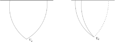
Figure 1: In the presence of a point source of baryon number there is a cusp singularity as shown on the left. When we have two branes and $SU(2)$ breaking source charge the branes separate. In the second figure the mirror D8 branes are not shown in detail but are indicated by a dotted line. Their configuration is chosen to satisfy the force balance condition.

From the bulk perspective adding a point source baryon charge, corresponding to the overall U(1), to the Sakai-Sugimoto model makes the D8 branes have a cusp geometry [34] (see Figure (1)).

The coupling of this point charge to the $U(1)$ gauge field on the brane is via a Chern-Simons term in the action via a point like instanton configuration. The instanton can also be understood as a D4 brane wrapped around the $S^{4}$ and has the same action [20]. However the instanton coupling requires more than one brane since it is a configuration involving non Abelian gauge fields. Thus we should interpret our single brane as a collection of $N_{d}$ coincident branes, with $N_{d}\geq 2$. The only role of the extra branes is to accommodate the instanton configuration. Otherwise as far as the rest of the dynamics that we are interested in is concerned, the collection behaves as one $U(1)$ brane. This $U(1)$ is the overall center of mass $U(1)$ in the $U(N_{d})$. All this is exactly as in [34].

In our case the new thing is that we have two such D8 branes with a $U(1)$ charge and Chern Simons term for each brane. Thus we have a $U(2)$ gauge symmetry on the branes. When the charges on the two branes are unequal then the branes come in at different angles and separate. The $U(2)$ symmetry is broken (Higgsed) to $U(1)\times U(1)$ when the branes are separated. These can be denoted as $U(1)_{B}\times U(1)_{3}$. $U(1)_{B}$ is the overall $U(1)$ of the $U(2)$ and $U(1)_{3}$ corresponds to the generator $t_{3}$ of the $SU(2)$.

We define the $SU(2)$ generators $(t_{+},t_{-},t_{3})\;$:

$$t_{+}=\left(\begin{array}[]{cc}0&1\\ 0&0\end{array}\right)~{}~{}~{}~{}~{}~{}t_{-}=\left(\begin{array}[]{cc}0&0\\ 1&0\end{array}\right)~{}~{}~{}~{}~{}~{}t_{3}=\frac{1}{2}\;\left(\begin{array}[]{cc}1&0\\ 0&-1\end{array}\right)$$ (1.3)

which satisfy the $SU(2)$ algebra

$$[t_{3},t_{\pm}]=\pm\;t_{\pm},~{}~{}~{}~{}[t_{+},t_{-}]=2\;t_{3}~{}~{}~{}~{}\{t_{+},t_{-}\}=I\;\;.$$

As mentioned above the Chern Simons coupling of each brane comes from having $N_{d}$ coincident branes. Thus we actually have $2N_{d}$ branes and a $U(2N_{d})$ symmetry. The $U(2)$ group that we are concerned with in this paper is thus embedded in an obvious way in the $U(2N_{d})$ group. (The mathematical description of this embedding is given for completeness in Appendix B.) The brane configuration thus leaves unbroken a $U(1)_{B}\times SU(N_{d})\times U(1)_{3}\times SU(N_{d})$ group.

From the bulk brane dynamics also we expect a condensate, because it is known that when branes intersect at an angle, in general there are tachyonic excitations [39, 40, 41]. Thus there should be a condensate of charged fields. This should then correspond to the Cooper pairing instability of the boundary theory. This generates a non zero electric field. In the presence of a non-zero electric field and charged condensate the tachyonic mode should get lifted and one expects a stable solution with electric field. This condensate breaks one more $U(1)$, namely $U(1)_{3}\;$, in the $U(1)_{B}\times SU(N_{d})\times U(1)_{3}\times SU(N_{d})$ group left unbroken by the geometric description of the D8 branes. As in [34] since the $SU(N_{d})\times SU(N_{d})$ gauge fields play no role in any of the dynamics we do not mention them again in the discussions below.

Figure 2: Tachyonic instability

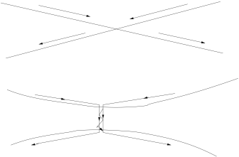
Figure 3: Electric field causes open strings to be formed that stabilize the configuration.

There is a geometric interpretation of the instability that makes this clear (see Figures 2, 3). The tachyonic mode corresponds to the tendency of the D branes to separate in the region around the intersection, and become parallel, because this reduces the energy. However, once there are open strings connecting the branes, it costs energy to separate the branes and make them parallel. Thus one expects stable solutions with condensates. We also expect to find analytic solutions in flat space describing charged condensates. The absence of tachyons in the presence of an electric field is confirmed by a perturbative analysis of the fluctuation spectra.

In fact there are solutions to the Yang-Mills equations that describe precisely such a situation: as soon as we have a non zero $t_{3}$ charge, there are solutions where $w^{\pm}$ fields condense. If the condensate extends to the boundary, we expect superconductivity in the boundary. We also give a proposal for calculating Greens functions in this situation. The complication here is that the branes do not extend all the way to the black hole. Hence the usual ingoing boundary conditions at the horizon cannot be applied because there is no horizon crossing. We apply this technique to the Sakai-Sugimoto model where Greens functions have not been calculated. We expect that the boundary fermions being massive the Green’s function (say, of the currents) should show a gap in the imaginary part. We find that the conductivity calculated using this prescription seems to have the expected properties. However we leave a detailed analysis to the future. Also applying to the BCS situation is more complicated and we have not attempted it in this paper.

We can summarize the above discussion as follows: In the bulk we have two (sets of coincident) D8 branes in the configuration shown in Figure 1. There are two $U(1)$ charges $d_{1},d_{2}$ corresponding to each brane. This can be represented as

$$\left(\begin{array}[]{cc}d_{1}&0\\ 0&d_{2}\end{array}\right)=d_{0}~{}{\mathbf{I}}+d_{3}~{}t_{3}=d_{0}\left(\begin{array}[]{cc}1&0\\ 0&1\end{array}\right)+{d_{3}\over 2}\left(\begin{array}[]{cc}1&0\\ 0&-1\end{array}\right)\;\;\;.$$ (1.4)

$d_{0}$ is the $U(1)_{B}$ baryon number charge and $d_{3}$ is the $U(1)_{3}$ (corresponding to $t_{3}$) charge. When $d_{3}>0$ the branes come in at different angles at the cusp $u_{c}$. For $u>>u_{c}$ the branes are parallel but separated by a finite distance. The $SU(2)$ is then broken to $U(1)_{3}$ as in the Georgi-Glashow model as soon as $d_{3}>0$. As long as no off diagonal $SU(2)$ fields are turned on the DBI action is exactly that of two independent branes and is easily analyzed. The free energy of this configuration can be studied for arbitrary values of $d_{0},d_{3}$.

We have also seen above that in this situation, a flat space analysis shows that there is a tachyonic instability which we plausibly identify with the BCS instability - assuming there are no other new unexpected boundary instabilities.

To quantitatively analyze this condensate in the D4 brane background we restrict ourselves to $d_{3}<<d_{0}$ and all $SU(2)$ fields smaller than the other terms in the DBI action. In this case it is consistent to expand the DBI action and keep the Yang-Mills part. A flat space analysis of Yang-Mills also tells us that there is a stable ground state where some charged fields condense. This encourages us to explore solutions of the Yang-Mills equations of motion in the D4 brane background. The curved space equations are then solved exactly, numerically and in some approximation analytically. There are solutions where the fields are small, validating the truncation of the DBI action to the leading Yang-Mills part. Also the existence of a charged condensate breaking the $U(1)_{3}$ symmetry implies that this approximation captures qualitatively the phenomenon that we are trying to describe. The smallness of the fields assures us that higher order terms can only change things quantitatively by small amounts - not qualitatively. Thus we have a self consistent scheme that gives us a ground state with a charged condensate. The $U(1)_{3}$ symmetry is broken. Thus we expect the same symmetry breaking in the boundary also. This is then identified with the BCS phenomenon.

One also expects that at finite temperature the positive $(mass)^{2}$ due to temperature effects will overwhelm the tachyonic tendency of the intersecting brane. The negative $(mass)^{2}$ is proportional to the angle between the branes, which in turn is fixed by the number density. So at a (dimensionless) $T_{c}$ roughly equal to the number density we expect superconductivity to disappear. This dependence on the power of number density is reminiscent of the strong coupling expression given earlier (for the gap). However we need a detailed calculation before anything concrete can be said. In any case it is very different from the weak coupling BCS expression.

This paper is organized as follows: In Section 2 we describe the brane solution in the presence of charges. In Section 3 we describe the Yang-Mills solution in flat space with $w^{\pm}$ condensate relevant for the D4-D8 case and analyze its stability In Section 4 we give the solutions (exact numerical and approximate analytic) again in the D4 background metric. This establishes the existence of a charged condensate. In Section 5 we study analytically the phase structure at zero temperature, i.e. as a function of chemical potential but without any condensate. With a condensate we give some numerical results.(The finite temperature analysis will be done elsewhere.) In Section 6 we give a sample calculation of a Greens function in the Sakai-Sugimoto model using a new prescription. We conclude in Section 7 with a discussion of our results and some open questions. The Appendices contain a collection of some useful results that are helpful in obtaining the equations.

2 Background Brane Configuration

The ten dimensional $D4$ brane background metric is

$$ds^{2}=\left({U\over R}\right)^{3\over 2}(\eta_{\alpha\beta}dy^{\alpha}dy^{\beta}+fd\theta^{2})+\left({R\over U}\right)^{3\over 2}\;({dU^{2}\over f}+U^{2}d\Omega_{4}^{2})$$

$$e^{\phi}=g_{s}\left({U\over R}\right)^{3\over 4},~{}~{}~{}~{}dC_{3}={2\pi N_{c}\over\Omega_{4}}\epsilon_{4},~{}~{}~{}~{}f=1-{U_{KK}^{3}\over U^{3}}$$ (2.1)

Here $y^{\alpha}(\alpha=0,1,2,3)$ and $\theta$ are the D4-brane directions. $d\Omega_{4}^{2}$ is the line element of $S^{4}$, $\epsilon_{4}$ is the volume form in 4 dimensions, and $\Omega_{4}={8\pi^{2}\over 3}$ is the volume of a unit 4-sphere. $C_{3}$ is the dual gauge field of the D4-brane and has components along $S^{4}\;$. $R^{3}=\pi g_{s}N_{c}l_{s}^{3}$ sets the scale of the space time curvature. $U_{KK}$ is related to the supersymmetry breaking scale, which is the period of the $\theta$ coordinate, ${4\pi\over 3}R^{3\over 2}\;U_{KK}^{-{1\over 2}}\equiv 2\pi Rr_{4}\;$.

One can define new dimensionless coordinates: $u={U\over R}$, $x^{\alpha}={y^{\alpha}\over R}$ and $\tau={\theta\over R}$, as well as a dimensionless gauge field: $a_{\mu}={2\pi\alpha^{\prime}\over R}A_{\mu}\;$. In these units, the period of the $\tau$ coordinate is ${4\pi\over 3}R^{1\over 2}\;U_{KK}^{-{1\over 2}}\equiv 2\pi r_{4}\;$, the metric becomes

$$ds^{2}=R^{2}\;[u^{3\over 2}(\eta_{\alpha\beta}dx^{\alpha}dx^{\beta}+fd\tau^{2})+u^{-{3\over 2}}\;({du^{2}\over f}+u^{2}d\Omega_{4}^{2})]$$

where $f(u)=1-{u_{KK}^{3}\over u^{3}}$ with $u_{KK}={U_{KK}\over R}\;$, and $e^{\phi}=g_{s}\;u^{3\over 4}\;$.

Our configuration consists of two flavor D8 branes with a background gauge field and some delta function sources. (As explained in the Introduction, these two D8 branes are actually two sets of $N_{d}$ number of coincident D8 branes.) The delta function sources correspond to baryons that are uniformly distributed in the $(x^{1},x^{2},x^{3})$ directions and at fixed $u=u_{c}\;$. Baryon number can come from D4 branes wrapped around $S^{4}$ and immersed in the D8 brane. They can equally well be thought of as an instanton background gauge field configuration of the non Abelian gauge field on the D8 brane. As shown by Sakai and Sugimoto, either picture yields the same value for the action.

The Chern-Simons action is (we have integrated by parts the action $C_{3}\wedge F\wedge F\wedge F$ and separated a $U(1)$ part for $A_{0}$)

$${1\over 16\pi^{2}}\int_{S^{4}}dC_{3}\int_{R^{4}}F\wedge F\int_{S^{1}}dt_{E}A_{0}$$

with $\int_{S^{4}}dC_{3}=2\pi N_{c}$ and $\int_{R^{4}}F\wedge F=8\pi^{2}N_{4}\int du\delta(u-u_{c})$ where we have assumed the instantons are localized at $u_{c}$.

As mentioned in the introduction even when we have one D8 brane we have to think of it as a set of coincident D8 branes with the associated non Abelian gauge fields providing the localized instanton configuration [34, 20]. These non Abelian fields are zero everywhere else and play no role in the rest of the dynamics. Thus we assume following Appendix B that $A=A^{a}\lambda^{a}+A\lambda^{0}$, where $\lambda^{a}$ are the Gell-Mann $\lambda$-matrices for $SU(3)$ and $\lambda^{0}$ is the $3\times 3$ identity matrix. The $SU(3)$ part of the gauge field is assumed to correspond to a localized instanton, so that $\int_{R^{4}}F\wedge F=8\pi^{2}N_{4}\int du\delta(u-u_{c})$. $A_{0}=A_{0}\lambda^{0}$ above is then assumed to be the $U(1)$ part.

When we have two $D8$ branes we assume two decoupled sets of the above, each with a $U(3)$ gauge group. The embedding of this $U(3)\times U(3)$ in $U(6)$ is given in Appendix B. As mentioned in the introduction, these $SU(3)$ fields play a role only in the Chern Simons action. They can be set to zero elsewhere. The effective DBI action is just a $U(2)$ non Abelian DBI action.

When the branes are separated, and the non-Abelian fields are not excited, this reduces to two decoupled Abelian DBI actions. In field theory language, we have a $U(1)\times SU(2)$ group broken to a $U(1)\times U(1)$. The Higgsing of the $SU(2)$ is by the adjoint field corresponding to the separation of the branes. This is just the Georgi-Glashow model. $U(1)\times U(1)$ can be denoted $U(1)_{B}\times U(1)_{3}$ as in (1.4). Thus $A=A_{B}{\mathbf{I}}+A_{3}t_{3}$.

We can factor out a 3-volume $V_{3}$ of the three dimensional space of the boundary theory, by writing $N_{4}=n_{4}{V_{3}\over R^{3}}\;$. $n_{4}$ is also dimensionless. In terms of these we get

$$S_{CS}={N_{c}N_{4}}\int dt_{E}A_{0}(u_{c})\equiv n_{B}\tilde{T}a_{0}(u_{c})$$ (2.2)

where, integrating over the Euclidean time $t_{E}$ with circumference $\beta$, we have

$$n_{B}\tilde{T}=N_{c}n_{4}{V_{3}\over R^{3}}\beta{R\over 2\pi\alpha^{\prime}}={N_{c}n_{4}V_{3}\beta\over R^{2}2\pi\alpha^{\prime}}\;\;.$$

The instanton number $N_{4}$ is thus the number of $D4$ branes and equivalently the number of baryons. The charge of a baryon is taken to be $N_{c}$.

The action of $N_{4}$ $D4$ branes wrapped on $S^{4}$ is

$$S_{D4}={1\over(2\pi)^{4}l_{s}^{5}}\int dt_{E}d^{4}\Omega\;e^{-\phi}\sqrt{-g_{00}g_{S^{4}}}={N_{4}R^{4}\Omega_{4}\beta\over(2\pi)^{4}l_{s}^{5}g_{s}}\;u_{c}$$

where we have integrated over the Euclidean time $t_{E}$ with circumference $\beta$. From the $u_{c}$ dependence we see that there is a downward force.

Using $N_{4}=n_{4}{V_{3}\over R^{3}}$, $g_{s}l_{s}^{3}={R^{3}\over N_{c}}$, and $\Omega_{4}={8\pi^{2}\over 3}$ we get for the D4-brane action:

$$S_{D4}={N_{c}n_{4}V_{3}\Omega_{4}\beta\over(2\pi)^{4}R^{2}l_{s}^{2}}u_{c}={n_{B}~{}\tilde{T}\over 3}u_{c}\;\;.$$ (2.3)

2.1 Solution of DBI action with source

The first step is to find the background $D8$ brane configuration. To this end we solve the equations of motion of the $D8$ brane Dirac-Born-Infeld action with a background gauge field on the $D8$ brane worldvolume.

$$S_{DBI}=-\tilde{T}\int d\sigma~{}{u^{5\over 2}\over\sqrt{f}}\;\;[u^{\prime 2}+u^{3}f^{2}\tau^{\prime 2}-f(\partial_{\sigma}a_{0})^{2}]^{1\over 2}-n_{B}\tilde{T}a_{0}(u_{c})$$ (2.4)

where $u^{\prime}=\partial_{\sigma}u\;$, $\tau^{\prime}=\partial_{\sigma}\tau\;$, $n_{B}$ was defined above and gives the magnitude of the charge to which $a_{0}$ couples, and $\tilde{T}={V_{3}R^{5}\Omega_{4}\over l_{s}^{9}g_{s}}$. Let

$$\Pi_{a}=\frac{u^{5\over 2}\;\sqrt{f}\;(\partial_{\sigma}a_{0})}{[u^{\prime 2}+u^{3}f^{2}\tau^{\prime 2}-f(\partial_{\sigma}a_{0})^{2}]^{1\over 2}}\;\;.$$

Then the equation of motion for $a_{0}$ is

$$\partial_{\sigma}\;\Pi_{a}={n_{B}}\;\delta(u-u_{c})\;\;.$$ (2.5)

Choose the coordinate $\sigma$ along the brane to be equal to $u$, the bulk radial coordinate. Then $u^{\prime}=1\;$ and $\tau^{\prime}=\partial_{u}\tau\;$.

Case 1: $n_{B}=0$

We then find in the absence of sources that $\Pi_{a}=d_{0}$, a constant. Thus,

$$\frac{u^{5}\;f\;(\partial_{u}a_{0})^{2}}{1+u^{3}f^{2}\tau^{\prime 2}-f(\partial_{u}a_{0})^{2}}=d_{0}^{2}$$ (2.6)

Solving for $\partial_{u}a_{0}$ we find

$$(\partial_{u}a_{0})^{2}={d_{0}^{2}\;(1+u^{3}f^{2}{\tau^{\prime}}^{2})\over f\;(u^{5}+d_{0}^{2})}$$ (2.7)

One can plug this back into the action and evaluate the Legendre transform of the Lagrangian density: $\tilde{\cal L}={\cal L}-~{}\tilde{T}\;\Pi_{a}\;\partial_{u}a_{0}\;$ :

$$\tilde{\cal L}(d_{0})=\tilde{T}\;\sqrt{u^{5}+d_{0}^{2}}\;\sqrt{{1\over f}+u^{3}f{\tau^{\prime}}^{2}}$$ (2.8)

We can repeat this for $\tau^{\prime}=\partial_{u}\tau$ and write the Legendre transformed Lagrangian density ${\cal L}(c_{0},d_{0})$:

$$\tilde{\cal L}(c_{0},d_{0})=-\tilde{T}\;{\sqrt{D}\over u^{3\over 2}f}$$ (2.9)

$$(\partial_{u}a_{0})^{2}={d_{0}^{2}\;u^{3}\over D}\;\;\;,\;\;\;\;(\partial_{u}\tau)^{2}={c_{0}^{2}\over u^{3}f^{2}D}$$ (2.10)

where $D=u^{8}f+d_{0}^{2}u^{3}f-c_{0}^{2}\;$. When $D\;$ vanishes (for some $u=u_{0}$), $\tau^{\prime}=\infty$. This is the lowermost point of the $D8-$brane and here the vertical force due to the brane tension vanish because the brane is horizontal. The horizontal forces cancel if we add a mirror $D8-$brane so that we have a symmetric U–shaped configuration. In the Sakai Sugimoto interpretation the second set of branes provide fermions of the opposite chirality, and are referred to as $\bar{D}8-$branes. The joining of these two sets of $D8-$branes represents the breaking of chiral symmetry.

Naively the gauge field strength diverges at $u_{0}$. However this is a “coordinate singularity” - the choice $\sigma=u$ is not good at $u=u_{0}$ because $\sigma$ keeps increasing monotonically as we proceed along the bottom of the U–shape, whereas $u$ starts to decrease again. See A. In this appendix a more general analysis is done keeping the coordinate $\sigma$ throughout. Thus $(\partial_{u}a_{0})={(a_{0})_{\sigma}\over u_{\sigma}}$ and $(\partial_{\tau}a_{0})={(a_{0})_{\sigma}\over\tau_{\sigma}}$ can be calculated for a given solution. The former is singular at $u_{0}$ because $u_{\sigma}$ vanishes at $u=u_{0}$, whereas the latter is finite. Calculating the latter can also be accomplished equivalently very simply by choosing $\sigma=\tau$ and investigating the same solution. One finds:

$$(\partial_{\tau}a_{0})^{2}={d_{0}^{2}u^{3}f\over d_{0}^{2}+u^{5}}\;\;.$$ (2.11)

Note that $u_{0}$ is a solution of $D(u_{0})=0\;$. So $u_{0}^{5}+d_{0}^{2}={c_{0}^{2}\over(u_{0}^{3}-u_{KK}^{3})}\;$. This gives

$$\partial_{\tau}a_{0}|_{u=u_{0}}={d_{0}^{2}\over c_{0}^{2}}\;(u_{0}^{3}-u_{KK}^{3})^{2}$$

which is finite.

In the absence of charges, continuity of flux would require that the electric field continue in the same direction along the other brane and reemerge on the boundary. Thus $\partial_{\sigma}a_{0}$ is continuous. On the other hand $\partial_{\tau}a_{0}$ changes sign because $\sigma=-\tau$ on the mirror brane. Since the equations above fix only the magnitude of $\partial_{\tau}a_{0}$, this is also a valid solution. The conclusion is that it is possible to have $d_{0}\neq 0$ even when $n_{B}=0$.

Case 2: $n_{B}\neq 0$

In this case there is a jump in the value of $\Pi_{a}$ at $u=u_{c}$. We will choose a solution where $\Pi_{a}=0$ for $u<u_{c}$ and equal to $n_{B}$ for $u>u_{c}$.

$$\partial_{u}\tau=\pm{c_{0}\over u^{3\over 2}f\;D}\;,~{}~{}~{}~{}~{}u>u_{c}$$ (2.12)

where $D=u^{8}f+n_{B}^{2}u^{3}f-c_{0}^{2}\;$. $u_{c}$ is determined by minimizing the action with respect to variations of $u_{c}$, subject to the constraint that

$$\int_{u_{c}}^{\infty}du~{}\tau^{\prime}={L\over 2}$$ (2.13)

$L$ is the distance between the $D8$ brane and the anti-$D8$ brane (assumed symmetric) at $u=\infty$. Note that the above constraint implies that

$$\int_{u_{c}}^{\infty}du~{}{d\tau^{\prime}\over du_{c}}-\tau^{\prime}(u_{c})=0$$ (2.14)

We work with $\tilde{S}(d)=-\tilde{T}\int_{u_{c}}^{\infty}du\sqrt{u^{5}+n_{B}^{2}}\sqrt{{1\over f}+u^{3}f\tau^{\prime 2}}$ for the D8 brane. The variation of $u_{c}$ gives the upward force due to the D8 brane tension. In order to get the downward force we (following [34, 35]) use the action of a D4 brane wrapped on $S^{4}\;$. The answer evaluated above is ${n_{B}\tilde{T}\over 3}u_{c}\;$. This gives a force of $n_{B}\tilde{T}\over 3\;$. We do not need a horizontal force balance as the mirror $\bar{D}8-$brane automatically provides the correct balancing force.

One can do the variation keeping either $L$ fixed or $c_{0}$ fixed. The latter is easier, since we just work with the Legendre transformed action:

$$-\tilde{T}\int_{u_{c}}^{\infty}{du\over u^{3\over 2}f}\;\sqrt{u^{8}f+n_{B}^{2}u^{3}f-c_{0}^{2}}$$ (2.15)

Varying $u_{c}$ just sets the integrand $\tilde{\cal L}(c_{0},n_{B})$ equal to $n_{B}\tilde{T}\over 3$, the force due to the D4-brane. One can solve for $u_{c}$ in terms of $c_{0},n_{B}$. The result for $c_{0}=100,u_{KK}=1$ is plotted in the figure.

If one substitutes for $c_{0}$ in terms of $\tau^{\prime}$ one can manipulate the D8-brane variation into the form:

$$\tilde{T}\;\;\underbrace{1\over u^{3\over 4}\sqrt{f}}_{\sqrt{g_{uu}}}\;\;\underbrace{u^{-{3\over 4}}\sqrt{u^{8}+u^{3}n_{B}^{2}}}_{tension}\;\;\underbrace{1\over\sqrt{1+u^{3}f^{2}\tau^{\prime 2}}}_{sin~{}\alpha}\;\;.$$

In this form it is easy to see the physical interpretation. The factor ($sin~{}\alpha$) gives the vertical component of the force. One also finds $sin^{2}\alpha_{c}={n_{B}^{2}\over u_{c}^{5}+n_{B}^{2}}$ where $\alpha_{c}$ is the angle with respect to the horizontal at $u=u_{c}\;$.

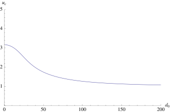
Figure 4: $u_{c}$ versus $d_{0}(=n_{B})$ with $c_{0}=100$

2.2 $SU(2)$ Breaking

Our aim is to introduce a finite “baryon number” corresponding to the $U(1)$ subgroup of $SU(2)$ generated by $t_{3}\;$. When this is done there are configurations of the type shown in the second diagram in Figure 1 where the two branes separate. The branes are parallel at large $u$, but separated by a finite distance. This Higgses the $SU(2)$ to $U(1)$ as in the Georgi-Glashow model.

The question is whether there will be a condensate that spontaneously breaks this $U(1)$ as happens in the BCS case. Note that on the boundary this is a global symmetry, so in this sense it is like superfluidity. However what is non trivial is that a fermion bilinear must condense in order for this symmetry to break. This is more like BCS than condensation of a bosonic field.

$u_{c}$ has a (rather complicated) dependence on $d_{0}(=n_{B})\;$ and $c_{0}\;$. Also, the angle of the brane depends on $n_{B}$. We have to choose values so that $u_{c}$ has the same value for both branes. Thus to begin with $c_{1}=c_{2};~{}~{}d_{1}=d_{2}\;$. We then turn on $d_{1}-d_{2}\;$, but change $c_{1},c_{2}$ such that $u_{c}$ remains the same. This can be done numerically.

Thus if we turn on a charge corresponding to $t_{3}$, which is the difference $n_{(3)}=n_{B1}-n_{B2}\;$, then we expect that the two branes will subtend different angles at $u_{c}\;$. Thus the situation is as shown in Figure (1). For small values of $n_{B}$ and the angle $\alpha_{c}\;$, $\alpha_{c1,d_{1}}-\alpha_{c2,d_{2}}\propto n_{B1}-n_{B2}=n_{(3)}\;$.

When two branes meet at an angle, in general there is a tachyonic mode. This mode corresponds to the tendency of the branes to smoothen out the angle and straighten out - see Figure (2) . In the presence of the electric field the situation is somewhat different. The presence of the electric field implies that there must be open strings which connect the two branes and carry the electric flux. The tension of these open strings then in principle can prevent the separation of the branes. In fact a perturbative stability analysis shows that there is no tachyon.

In general one expects the relation between the slope $\alpha_{c}$ and the electric field $n_{B}$ to be modified by the condensate. The condensation corresponds to $\phi^{\pm}$ and in general also $w^{\pm}$.

The background configuration breaks $SU(2)$ . The Non Abelian DBI action [42] is well defined as long as the background is diagonal, which means it lies in the $U(1)\times U(1)$ subgroup of $U(2)$. Otherwise there are ambiguities in the definition of the determinant . There is the symmetrized trace prescription that is often used, though in general it is known that there are modifications at the $O({\alpha^{\prime}})^{6}$[43, 44].

When the $SU(2)$ fields are small one can study this problem in the Yang-Mills approximation to the Dirac-Born Infeld. In Section 3 we give an exact solution of the Yang-Mills equations in flat space. This solution is not the most general. It has $\phi^{+}=0\;$, although $w^{+}\neq 0\;$. As a consequence the asymptotic slope is still fixed by the electric field.

In the presence of the D4 D8 background and the supersymmetry breaking metric function $f(u)\;$, we find an approximate solution of the Yang-Mills equations by neglecting some terms in the equation of motion. We find that at least when $u_{c}>>R_{AdS}$ the neglected terms are small and we expect our solution to be a good approximation. This is described in Section 4. To do better than this one needs a numerical solution. We give some exact numerical solutions in Section 4. The solutions where the $SU(2)$ fields are small a posteriori justify the Yang-Mills approximation and are thus very close to the exact solutions of the DBI action.

The conclusion is thus that as soon as we turn on a charge (corresponding to $t_{3}$) we have a solution where there is a charge violating condensate. This must be a reflection of the fact that from the boundary theory viewpoint, as soon as we have a Fermi surface (i.e. a non zero chemical potential) there is an instability towards a BCS phase.

As a caveat one should note that this analysis does not take into account the tachyon condensation that represents the fermion mass generation. However this should not affect the BCS instability, which only requires gapless excitation above the Fermi surface. The existence of this is not affected by the fermions being massive.

In the next section we analyze the stability of this solution in flat space using Yang-Mills as an approximation to Dirac-Born- Infeld.

3 The Yang-Mills Approximation

We will assume that the fields on the $D8$ brane depend only on $(t,u)\;$, thus keeping translational invariance in $(x^{1},x^{2},x^{3})\;$. The $S^{4}$ coordinate dependence is also not assumed. The $D8$ brane has only one transverse direction, $\tau$, which we call $\phi$ here. The index $\mu$ on the Yang-Mills gauge field $A_{\mu}$ has nine values. However, we set $A_{\mu}=0$ along the four directions of the $S^{4}\;$. For the stability analysis we concentrate on $A_{0},A_{u}$ and $\phi$. For other purposes, such as calculating correlators of the boundary theory, we also use $A_{x^{1}}$.

We define the $SU(2)$ generators $(t_{+},t_{-},t_{3})\;$:

$$t_{+}=\left(\begin{array}[]{cc}0&1\\ 0&0\end{array}\right)~{}~{}~{}~{}~{}~{}t_{-}=\left(\begin{array}[]{cc}0&0\\ 1&0\end{array}\right)~{}~{}~{}~{}~{}~{}t_{3}=\frac{1}{2}\;\left(\begin{array}[]{cc}1&0\\ 0&-1\end{array}\right)$$ (3.1)

which satisfy the $SU(2)$ algebra

$$[t_{3},t_{\pm}]=\pm\;t_{\pm},~{}~{}~{}~{}[t_{+},t_{-}]=2\;t_{3}~{}~{}~{}~{}\{t_{+},t_{-}\}=I\;\;.$$

If we write $A=A^{+}t_{+}+A^{-}t_{-}+A^{3}t_{3}\;$ then $Tr(AA)={1\over 2}[(A^{3})^{2}+4A^{+}A^{-}]\;$.

In this basis we define the Yang-Mills field $A_{\mu}=A^{+}_{\mu}t_{+}+A^{-}_{\mu}t_{-}+A^{3}_{\mu}t_{3}\;$ and, similarly, an adjoint scalar field $\phi=\phi^{+}t_{+}+\phi^{-}t_{-}+\phi^{3}t_{3}\;$ where $\phi^{3}$ is real and $\phi^{\pm}$ are complex conjugates of each other. The covariant derivative is defined by

$$D_{\mu}\phi=\partial_{\mu}\phi+i[A_{\mu},\phi]$$

and the field strength by

$$F_{\mu\nu}=\partial_{\mu}A_{\nu}-\partial_{\nu}A_{\mu}+i[A_{\mu},A_{\nu}]\;\;.$$

We can write the Yang-Mills and scalar field action as

$$S=-{1\over 2}Tr[F_{\mu\nu}F^{\mu\nu}]-Tr[D_{\mu}\phi D^{\mu}\phi]\;\;.$$ (3.2)

3.1 Solutions of the Equations of Motion

We first study the case where the background space time is flat. Later, we will study the case where the background space time is curved.

3.1.1 Solution with $A_{\mu}=0$

The simplest non trivial solution is of course the Higgs phase where $\phi^{3}=const$. The resulting unbroken symmetry is just $U(1)\;$. In the brane language this corresponds to a constant separation of the $D8$ branes in the $\tau$ direction.

The configuration of intersecting $D8$ branes corresponds, in the Yang-Mills description to having $\phi=qut_{3}\;$ where $q$ is the slope. Clearly this satisfies the equations of motion

$$D^{\mu}D_{\mu}\phi=0\;\;,\;\;\;D^{\mu}F_{\mu\nu}=[\phi,D_{\nu}\phi]$$

where $D_{\mu}(*)=\partial_{\mu}(*)+i[A_{\mu},(*)]\;$. For the given configuration $D_{u}\phi$ is constant and $A_{\mu}$ is zero, so it clearly satisfies the equations of motion.

When we embed $D8$ branes in $D4$ brane background, as the discussion in the previous section shows, there are solutions that interpolate between these two solutions. However this requires a non zero $A_{0}$.

3.1.2 Solutions with $A_{0}\neq 0$

We can have a configuration where $A_{0}^{3}=-Eu\;$, in addition to the above $\phi\;$. This corresponds to a constant electric field $E$ and also clearly satisfies the equations of motion. It is this solution (near $u=u_{c}$) that interpolates with the $\phi=const$ solution near $u=\infty\;$, in the $D4$ background.

Solution I:

We choose a gauge where $A_{0}^{\pm}=A_{u}^{3}=0\;$. By imposing this everywhere including the boundary, we are freezing the Goldstone modes (pions) [23]. We consider time independent configurations and also set the charged scaler to zero. We list below the various equations, after the choice of gauge :

The equations are:

$$\partial_{u}^{2}A^{3}_{0}-4w^{+}w^{-}A^{3}_{0}=0$$ (3.3)

$$\partial_{u}^{2}\phi^{3}-4w^{+}w^{-}\phi^{3}=0$$ (3.4)

$$\partial_{u}(w^{+}A^{3}_{0})+w^{+}\partial_{u}A^{3}_{0}=0$$ (3.5)

$$((A^{3}_{0})^{2}-(\phi^{3})^{2})\;w^{+}=0$$ (3.6)

$$\partial_{u}(w^{+}\phi_{3})+w^{+}\partial_{u}\phi_{3}=0$$ (3.7)

Eqn (3.5) implies that $(A_{0}^{3})^{2}w^{+}=c$, where is $c$ is a constant. Clearly $\phi^{3}=A_{0}^{3}$ is required too. Finally plugging into (3.3), Gauss law, we can integrate to get

$$A_{0}^{3}(u)=\phi^{3}(u)=\sqrt{{du^{2}\over 4}+{4c\over d}};~{}~{}~{}~{}~{}~{}w^{+}=w^{-}={c\over{du^{2}\over 4}+{4c\over d}}$$ (3.8)

The D8 brane has the expected profile - the intersection region is smoothed out, but it does not straighten out fully, and there is a condensate of $w^{\pm}$ representing open strings connecting the two D8 branes. This solution was also studied in [46].

Solution II:

A solution can also be obtained if there are two adjoint scalars $\phi_{1}$ and $\phi_{2}\;$, with the action given by

$$S=-{1\over 2}Tr[F_{\mu\nu}F^{\mu\nu}]-Tr[D_{\mu}\phi_{1}D^{\mu}\phi_{1}]-Tr[D_{\mu}\phi_{2}D^{\mu}\phi_{2}]+Tr[\phi_{1},\phi_{2}]^{2}\;\;.$$ (3.9)

We define

$$\chi = \chi^{3}t_{3}+\chi^{+}t_{+}+\chi^{-}t_{-}\equiv\phi_{1}+i\phi_{2}$$

$$= (\phi_{1}^{3}+i\phi_{2}^{3})t_{3}+(\phi_{1}^{+}+i\phi_{2}^{+})t_{+}+(\phi_{1}^{-}+i\phi_{2}^{-})t_{-}$$

and, in an obvious way,

$$\chi^{*} = (\chi^{3})^{*}t_{3}+(\chi^{+})^{*}t_{+}+(\chi^{-})^{*}t_{-}\equiv\phi_{1}-i\phi_{2}$$

$$= (\phi_{1}^{3}-i\phi_{2}^{3})t_{3}+(\phi_{1}^{+}-i\phi_{2}^{+})t_{+}+(\phi_{1}^{-}-i\phi_{2}^{-})t_{-}\;\;,$$

and, finally,

$$\bar{\chi}\equiv(\chi^{*})^{T}=(\chi^{3})^{*}t_{3}+(\chi^{+})^{*}t_{-}+(\chi^{-})^{*}t_{+}\;\;.$$

Thus $\bar{\chi}^{+}=(\chi^{-})^{*}\;$, $\;\bar{\chi}^{-}=(\chi^{+})^{*}\;$, and $\;\bar{\chi}^{3}=(\chi^{3})^{*}\;$.

Of course if we set $\chi=0$ we have the same solution as before. Furthermore, if we set one of the scalar fields, such as $\phi_{1}=0\;$, then the system is again the earlier one and we only have an analytic solution where $\phi_{2}$ is also zero. So we try to set a different set to zero. One can try for instance to set $\phi_{1}^{3}=0=\phi_{2}^{\pm}\;$

The equations and details of the solution are given in the Appendix F.

When all the dust settles we find that $\chi^{+}$ can be nonzero: either a constant or linear in $u$. But this changes fairly dramatically the behavior of $A_{0}^{3}$ - it becomes exponential rather than linear. If we take $\chi^{+}=\chi_{0}=constant$ then $A_{0}^{3}$ can be solved for in closed form: One finds using the same methods as earlier

$$A_{0}^{3}(u)=\sqrt{a\chi_{0}}\;cosh~{}(\chi_{0}\;u)$$ (3.10)

Note that $\partial_{u}A^{3}_{0}(0)=0\;$, and thus the electric field vanishes at $u=0$ as required by symmetry.

3.2 Stability

In this section we study the stability of the solutions given in the last section. The stability of the solution with linear $\phi^{3}$ has been analyzed by [41, 45, 46, 47] and as mentioned earlier a tachyon was found. This tachyonic instability is illustrated in Figure 2.

The instability would continue till the initially intersecting branes straighten out completely, if we take this linearized picture seriously. However what actually happens is more complex. The condensing tachyon is a charged field. Once there are charges one has to take into account electric fields. The situation when there is an electric field present is described in Figure 3. Since the electric fields point in opposite directions on the two branes (we are considering the $U(1)$ generated by $t_{3}$ of $SU(2)$), as the branes separate open strings need to be formed to carry the electric flux. These open strings between the separating branes have tension, oppose stretching, and do not want to stretch beyond a point. This stabilizes the configuration.

This intuitive picture is consistent with the linearized stability analysis given below: One finds that $(mass)^{2}={(q^{2}-E^{2})^{3\over 2}\over q^{2}}\;(2n+1)\;$ when $q^{2}>E^{2}>0\;$, and $(mass)^{2}=(2n-1)\;|q|$ when $E=0\;$, with $n=0,1,2,\cdots\;$. Thus, the lowest $(mass)^{2}\propto(q^{2}-E^{2})^{3\over 2}>0$ when $E\neq 0\;$, and the lowest $(mass)^{2}<0$ when $E=0\;$.

The $N_{f}=2\;$ number of $D8$ branes in our case are in a background space curved by the $D4$ branes. Nevertheless near the cusp at $u=u_{c}\;$, where these two $D8$ branes intersect, the local physics can be studied using the flat space model. This is what is done below.

The equations for small fluctuations is derived in the Appendix G.

Let us assume $\phi^{+}(t,u)=\phi(u)\;e^{-imt}\;$ and $w^{+}(t,u)=iw(u)\;e^{-imt}\;$. Using $\phi^{3}=qu$ and $A^{3}_{0}=-Eu\;$, we then get

$$\partial_{u}^{2}\phi+q\;(2+u\partial_{u})w+(m+Eu)^{2}\phi=0$$ (3.11)

$$(q^{2}u^{2}-(m+Eu)^{2})w=q(1-u\partial_{u})\phi$$ (3.12)

Define

$$b^{2}=q^{2}-E^{2}\;\;,\;\;\;c=\frac{m^{2}q^{2}}{b^{2}}\;\;,\;\;\;\tilde{u}=u-\frac{mE}{b^{2}}$$

and the functions $P(u)\;$ and $Q(u)\;$ by

$$P(u)=\frac{2mq^{2}}{(m+Eu)\;Q(u)}\;\;\;,\;\;\;\;\;Q(u)=q^{2}u^{2}-(m+Eu)^{2}=b^{2}\tilde{u}^{2}-c\;\;.$$

Then using (3.12) the equation (3.11) becomes

$$\partial_{u}^{2}\phi-uP\;\partial_{u}\phi-(Q-P)\;\phi\;=\;0\;\;.$$ (3.13)

For large $u\;$, we have $uP\sim 0\;$, $P\sim 0\;$, and $Q\sim b^{2}u^{2}\;$. So, asymptotically for large $u\;$, this is a Schrödinger equation for harmonic oscillator. Let $\phi=e^{-\frac{b}{2}\tilde{u}^{2}}F\;$ where $b=\sqrt{q^{2}-E^{2}}\;>0\;$ and $\tilde{u}\;$ has been defined earlier. We then have

$$\partial_{u}^{2}F-(2b\tilde{u}+uP)\;\partial_{u}F+(c-b+(1+bu\tilde{u})P)\;F\;=\;0\;\;.$$ (3.14)

Letting $F(u)=u^{n}\;$, where $n\geq 0\;$ is an integer, and noting that $P\sim\frac{1}{u^{3}}\;$ for large $u\;$, we get from the coefficient of $u^{n}$ the eigenvalue condition: $c=(2n+1)\;b\;$, which shows that $m^{2}={(q^{2}-E^{2})^{3\over 2}\over q^{2}}\;(2n+1)\;$ is always non-negative. When $q^{2}=E^{2}\;$, the spectrum is gapless.

This is to be contrasted with the situation where $E=0\;$. Observe that $P\sim\frac{2mq^{2}}{b^{2}E}\;\frac{1}{u^{3}}\;$ for large $u\;$ if $E\neq 0\;$, irrespective of how small $|E|$ is. But, if $E=0$ exactly then $P\sim\frac{2q^{2}}{b^{2}}\;\frac{1}{u^{2}}\;$ for large $u\;$. This results in the $(bu\tilde{u}PF)-$term contributing to the eigenvalue condition which is now: $c=(2n+1)\;b-\frac{2q^{2}}{b}$ which gives $m^{2}=(2n-1)\;|q|$ since $b=|q|$ and $c=m^{2}$ when $E=0\;$. This condition reveals the presence of a tachyonic mode when $E=0\;$.

The new solution with $w^{\pm}\neq 0$, described in the last section has the same asymptotics as the above solution, hence we do not expect a tachyon. Nevertheless, since $q=E$, there are massless modes and so we expect that there are continuous deformations. This is certainly true since the solutions are characterized by integration constants $(c,d)\;$ which are free parameters and can be changed continuously.

Finally, the fact that the negative $(mass)^{2}$ is proportional to the angle, which in turn, is proportional to the number density, suggests that the critical temperature at which superconductivity is lost is proportional to a power of the number density. This is different from the usual BCS relation and is closer to the strong coupling BCS result given in the Introduction.

4 Solutions in Curved Space Time

In this section we give the curved space counterparts of the flat space equations given in Section 3.1. We also attempt to find a solution that is the counterpart of the one presented there. Our aim will be to establish in a qualitative way that the flat space solutions presented in Section 3.1 have a generalization to the $D4D8$ background. A quantitative (numerical) study of these equations is not attempted in this paper.

4.1 Equations of Motion

Our starting point is the Dirac-Born-Infeld action, with $\sigma=u\;$,

$$S_{DBI}=-\tilde{T}\int d^{4}x~{}du~{}{u^{5\over 2}\over\sqrt{f}}\;\;[1+u^{3}f^{2}\tau^{\prime 2}-f(\partial_{u}a_{0})^{2}]^{1\over 2}-n_{B}\tilde{T}a_{0}(u_{c})$$ (4.1)

For the moment we ignore the source term. We have

$$[1+u^{3}f^{2}\tau^{\prime 2}-f(\partial_{u}a_{0})^{2}]^{1\over 2}\approx 1+{1\over 2}u^{3}f^{2}\tau^{\prime 2}-{1\over 2}f(\partial_{u}a_{0})^{2}\;\;.$$ (4.2)

The last two terms are nothing but ${1\over 2}g^{uu}g_{\tau\tau}(\partial_{u}\tau)^{2}+{1\over 2}g^{00}g^{uu}f_{0u}^{2}$ which are the world volume scalar kinetic term $g_{\tau\tau}\;\partial_{\mu}\tau\partial^{\mu}\tau\;$ and the Maxwell term $f_{\mu\nu}f^{\mu\nu}\;$ written in curved space-time. The factor $g_{\tau\tau}$ is a component of the background space–time metric in the transverse direction.

For the case of two D8 branes, we need the non-Abelian Dirac-Born-Infeld action [42]. However this is not very well defined although there are prescriptions that are known to be consistent up to some order [43, 44]. We will bypass this complication by expanding the Dirac-Born-Infeld action as was done above and using the Yang-Mills approximation for the non Abelian gauge field $A_{\mu}\;$ and keeping the Dirac-Born-Infeld structure for the $U(1)$ gauge field $a_{\mu}\;$. In order to get the correct normalization of the the commutator term $[A_{0},\tau]^{2}$ we will start with a $U(1)$ theory that has time derivatives of $\tau\;$, covariantize and then set the time derivative to zero. See C and D also.

Thus our starting point is:

$$[(g_{00}+g_{\tau\tau}\dot{\tau}^{2})(g_{uu}+g_{\tau\tau}\tau^{\prime 2})+f_{0u}^{2}]^{1\over 2}$$

$$=[g_{00}g_{uu}(1+g^{00}g_{\tau\tau}{\dot{\tau}}^{2})(1+g^{uu}g_{\tau\tau}{\tau^{\prime}}^{2}))+f_{0u}^{2}]^{1\over 2}$$

$$=[g_{00}g_{uu}((1+g^{00}g_{\tau\tau}{\dot{\tau}}^{2})(1+g^{uu}g_{\tau\tau}{\tau^{\prime}}^{2})+g^{00}g^{uu}f_{0u}^{2})]^{1\over 2}$$

$$=[g_{00}g_{uu}((1+g^{uu}g_{\tau\tau}{\tau^{\prime}}^{2}+g^{00}g^{uu}f_{0u}^{2})+(1+g^{uu}g_{\tau\tau}{\tau^{\prime}}^{2})g^{00}g_{\tau\tau}{\dot{\tau}}^{2})]^{1\over 2}$$

Covariantize now $\dot{\tau}$ and set the time derivative to zero : $\dot{\tau}\rightarrow D_{0}\tau\rightarrow i[A_{0},\tau]\;$. This gives:

$$S_{DBI}=-\tilde{T}\int d^{4}x~{}du~{}{u^{5\over 2}\over\sqrt{f}}\;\sqrt{X}\;-\;n_{B}^{U(1)}a_{0}(u_{c})\;-\;\vec{n}_{B}^{SU(2)}\cdot\vec{A}_{0}(u_{c})$$ (4.3)

where $X$ is given, denoting the $SU(2)$ part of $\tau$ by $\phi\;$, by

$$X\equiv 1+g^{uu}g_{\tau\tau}[\tau^{{}^{\prime}2}+2Tr({D_{u}\phi})^{2}]+\;g^{00}g^{uu}[(\partial_{u}a_{0})^{2}+2\;Tr(F_{0u})^{2}]$$

$$+(1+g^{uu}g_{\tau\tau}\tau^{\prime 2})g^{00}g_{\tau\tau}\;2Tr(i\;[A_{0},\phi])^{2}$$

Note that the factor of 2 for $SU(2)$ traces is because the $t_{3}$ generator is defined to be ${1\over 2}\tau_{3}$ where $\tau_{3}$ is the Pauli matrix.

For the $SU(2)$ part, the covariant derivative $D_{\mu}*=\partial_{\mu}*+i[A_{\mu},*]$ has been introduced in place of the ordinary derivative, and $F_{\mu\nu}=\partial_{\mu}A_{\nu}-\partial_{\nu}A_{\mu}+i[A_{\mu},A_{\nu}]$ is the non-Abelian field strength. Had the $SU(2)$ fields been entirely in the diagonal $t_{3}$ direction, this action would have been exact. This was discussed in Section 1. To the extant that there are off diagonal terms, this action is not correct. It can also be shown that if the off diagonal terms are entirely in the antisymmetric $F_{0u}$ part, then the symmetrized trace prescription gives exactly this action. (A proof is given in the C). Since the symmetrized trace prescription is itself known to be correct only up to $O((\alpha^{\prime})^{6})$ we will not belabor this point here. However we assume for the moment that the off diagonal terms are small and work with this action and expand the $SU(2)$ part in the square root keeping the background $U(1)$ inside the square root.

Defining $\Delta=1+g_{\tau\tau}g^{uu}\tau^{{}^{\prime}2}+g^{00}g^{uu}(\partial_{u}a_{0})^{2}\;$, we have

$$S_{DBI}\approx-\tilde{T}\int d^{4}x~{}du~{}{u^{5\over 2}\over\sqrt{f}}\;\sqrt{\Delta}\;[1+{1\over 2\Delta}\;[g^{uu}g_{\tau\tau}\;2Tr(D_{u}\phi)^{2}$$

$$+(1+g^{uu}g^{00}\tau^{\prime 2})g^{00}g_{\tau\tau}\;2Tr(i[A_{0},\phi])^{2}+g^{00}g^{uu}\;2Tr(F_{0u})^{2}]\;]$$

$$=\tilde{T}\int d^{4}x~{}du~{}[{u^{5\over 2}\over\sqrt{f}}\;\sqrt{\Delta}\;+\underbrace{u^{5\over 2}\over\sqrt{f\;\Delta}}_{{\rm``}\;\sqrt{-g}\;"}\;[g^{uu}g_{\tau\tau}Tr(D_{u}\phi)^{2}$$

$$+\;(1+g^{uu}g^{00}\tau^{\prime 2})g^{00}g_{\tau\tau}Tr(i[A_{0},\phi])^{2}+g^{00}g^{uu}Tr(F_{0u})^{2}\;]\;]\;\;.$$ (4.4)

The pre factor multiplying the Yang-Mills action has been denoted symbolically as $\sqrt{-g}$.

Note that if we had $g^{\tau\tau}$ instead of $g_{\tau\tau}$, then in the limit $f=1$ the scalar could have been thought of as another vector and the action would be the same as the flat space action up to an overall factor. It is easy to see that in this case the flat space solution given in the last section can be generalized very directly to curved space.

We are interested in static and translation invariant (in the $(x^{1},x^{2},x^{3})$ directions) solutions of the equations of motion. The fields thus depend only on $u$. The equations are the following. These equations assume that $\tau^{\prime}=0\;$, i.e. neglect the bending of the D8 branes.

$${\delta S\over\delta A^{3}_{0}}=-\partial_{u}\;(\sqrt{-g}g^{00}g^{uu}\partial_{u}A^{3}_{0})+4\;\sqrt{-g}g^{00}\;(g^{uu}w^{+}w^{-}+g_{\tau\tau}\phi^{+}\phi^{-})\;A^{3}_{0}$$

$${\delta S\over\delta A^{3}_{1}}=2i\;\sqrt{-g}g^{uu}g_{\tau\tau}\;(\phi^{-}D_{u}\phi^{+}-\phi^{+}D_{u}\phi^{-})$$

$${\delta S\over\delta\phi^{3}}=\partial_{u}(\sqrt{-g}g^{uu}g_{\tau\tau}D_{u}\phi^{3})-2i\;\sqrt{-g}g^{uu}g_{\tau\tau}\;(w^{-}D_{u}\phi^{+}-w^{+}D_{u}\phi^{-})$$

$${\delta S\over\delta A^{-}_{0}}=2i\;\partial_{u}\;(\sqrt{-g}g^{00}g^{uu}w^{+}A^{3}_{0})+2i\;\sqrt{-g}g^{00}g^{uu}w^{+}\partial_{u}A^{3}_{0}-2\sqrt{-g}g^{00}g_{\tau\tau}A^{3}_{0}\phi^{3}\phi^{+}$$

$${\delta S\over\delta A^{-}_{1}}=2i\;\sqrt{-g}g^{uu}g_{\tau\tau}\;(\phi^{+}D_{u}\phi^{3}-\phi^{3}D_{u}\phi^{+})-2\sqrt{-g}g^{00}g^{uu}\;(A^{3}_{0})^{2}w^{+}$$

$${\delta S\over\delta\phi^{-}}=2\partial_{u}\;(\sqrt{-g}g^{uu}g_{\tau\tau}D_{u}\phi^{+})-2i\;\sqrt{-g}g^{uu}g_{\tau\tau}w^{+}D_{u}\phi^{3}-2\sqrt{-g}g^{00}g_{\tau\tau}(A^{3}_{0})^{2}\phi^{+}$$ (4.5)

where

$$D_{u}\phi^{3}=\partial_{u}\phi^{3}-2i\;(w^{-}\phi^{+}-w^{+}\phi^{-})\;\;\;,\;\;\;\;D_{u}\phi^{+}=\partial_{u}\phi^{+}-iw^{+}\phi^{3}\;\;.$$

Here, we note the following. Let $\phi^{\pm}=\phi\;e^{\pm i\theta}\;$ and $w^{\pm}=w\;e^{\pm i\Omega}\;$ where $\phi$ and $w$ are real. It then follows from ${\delta S\over\delta A^{3}_{1}}$ and ${\delta S\over\delta A^{-}_{1}}$ equations above that $\Omega=\theta+\frac{\pi}{2}=constant\;$.

As mentioned above if we replace $g_{\tau\tau}$ by $g^{\tau\tau}$ and set $f(u)=1$ (which is a good approximation if $u>>u_{KK}$), then one can set $\phi^{+}=0$ as in flat space and recover the same solution. Thus one would get $\sqrt{-g}\;(A^{3}_{0})^{2}w^{+}=\sqrt{-g}\;(\phi^{3})^{2}w^{+}=const$, which except for the factor $\sqrt{-g}$ is exactly as in flat space. But $g_{\tau\tau}=u^{3\over 2}$, so clearly one cannot do this. However this suggests a change of variables: Introduce auxiliary fields $\psi^{a}$ satisfying: $g_{\tau\tau}D_{u}\phi^{a}=g^{\tau\tau}D_{u}\psi^{a}\;$. In all the equations where $\phi^{a}$ enter linearly, this change gets rid of $\phi^{a}$ and those equations look exactly like the flat space case. However where $\phi^{a}$ enter quadratically, one ends up with both $\phi^{a}$ and $\psi^{a}\;$. This happens in the gauge field variations. However, since $D_{u}\phi^{a}=(g^{\tau\tau})^{2}\;D_{u}\psi^{a}=u^{-3}\;D_{u}\psi^{a}\;$, one expects that $D_{u}\phi^{a}$ are very small compared to $D_{u}\psi^{a}\;$ for large $u\;$. It is plausible that terms involving $\phi^{a}$ are much smaller than the other terms, at least for very large $u\;$. Thus our strategy will be to set these terms to zero as the zeroth approximation. The equations of motion can now be solved analytically for $\psi^{a}\;$. In terms of $\psi^{a}$ one can solve for $\phi^{a}\;$. In the case where we set $\Delta=1\;$, this can in fact be done analytically, though only a numerical solution is possible in general. One can now verify whether there is some range of parameters where the neglected terms are really small, so that we have a self consistent procedure. We do find for very large $u\approx 1000$ and specific values of the parameters, the correction terms are a few percent of the terms we keep.

We give the substituted equations below. The terms involving $\phi^{a}\;$ which are supposedly small are in boldface.

$${\delta S\over\delta A^{3}_{0}}=-\partial_{u}\;(\sqrt{-g}\partial_{u}A^{3}_{0})+4\sqrt{-g}A^{3}_{0}w^{+}w^{-}+\boldsymbol{4\sqrt{-g}\phi^{-}\phi^{+}A^{3}_{0}}$$ (4.6)

$${\delta S\over\delta A^{3}_{1}}=2i\;\sqrt{-g}\;(\phi^{-}\partial_{u}\psi^{+}-\phi^{+}\partial_{u}\psi^{-})+2\sqrt{-g}\;(\phi^{-}w^{+}+\phi^{+}w^{-})\;\psi^{3}$$ (4.7)

$${\delta S\over\delta\phi^{3}}=\partial_{u}\;(\sqrt{-g}\partial_{u}\psi^{3})-2i\partial_{u}\;(\sqrt{-g}(\psi^{+}w^{-}-\psi^{-}w^{+}))$$

$$-2i\;\sqrt{-g}\;(w^{-}\partial_{u}\psi^{+}-w^{+}\partial_{u}\psi^{-})-4\;\sqrt{-g}\;w^{+}w^{-}\;\psi^{3}$$ (4.8)

$${\delta S\over\delta A^{-}_{0}}=2i\;\partial_{u}\;(\sqrt{-g}w^{+}A^{3}_{0})+2i\;\sqrt{-g}\;w^{+}\partial_{u}A^{3}_{0}-\boldsymbol{2\;\sqrt{-g}\;A^{3}_{0}\phi^{3}\phi^{+}}$$ (4.9)

$${\delta S\over\delta A^{-}_{1}}=-2\;\sqrt{-g}\;((A^{3}_{0})^{2}-\phi^{3}\psi^{3})\;w^{+}+\boldsymbol{2i\sqrt{-g}(\phi^{+}\partial_{u}\psi^{3}-\phi^{3}\partial_{u}\psi^{+})}$$

$$+\boldsymbol{4\sqrt{-g}\phi^{+}(\psi^{+}w^{-}-\psi^{-}w^{+})}$$ (4.10)

$${\delta S\over\delta\phi^{-}}=2\;\partial_{u}\;(\sqrt{-g}\;\partial_{u}\psi^{+})-2i\;\partial_{u}\;(\sqrt{-g}\;w^{+}\psi^{3})-2i\;\sqrt{-g}\;w^{+}\partial_{u}\psi^{3}$$

$$-4\;\sqrt{-g}\;(w^{-}\psi^{+}-w^{+}\psi^{-})\;w^{+}-\boldsymbol{2\sqrt{-g}(A^{3}_{0})^{2}\phi^{+}}$$ (4.11)

Equation (4.7) can be satisfied identically by the reality conditions: $\phi^{\pm}=\pm\;i\;\phi(u)\;$, $\;\psi^{\pm}=\pm\;i\;\psi(u)$ and $w^{\pm}=w(u)\;$. The following configurations solve the equations (4.6, 4.8, 4.9, 4.11), when the terms in bold are neglected:

$$A^{3}_{0}=\sqrt{{D_{A}G(u)^{2}\over 2}+{2C_{A}^{2}\over D_{A}}}\;\;\;,\;\;\;\;\sqrt{-g}(A^{3}_{0})^{2}\;w(u)=C_{A}$$

$$\psi^{3}=\sqrt{{D_{3}G(u)^{2}\over 2}+{2C_{3}^{2}\over D_{3}}}\;\;\;,\;\;\;\;\sqrt{-g}(\psi^{3})^{2}\;w(u)=C_{3}$$

$$\psi=\sqrt{{D_{+}G(u)^{2}\over 2}+{2C_{+}^{2}\over D_{+}}}\;\;\;,\;\;\;\;\sqrt{-g}(\psi^{+})^{2}\;w(u)=C_{+}$$ (4.12)

where $G(u)-G(u_{c})=\int^{u}_{u_{c}}du^{\prime}\;{2\over\sqrt{-g(u^{\prime})}}\;\;$. The above equations imply that

$${D_{A}\over C_{A}}={D_{3}\over C_{3}}={D_{+}\over C_{+}}\;\;.$$ (4.13)

Given $\psi^{a}$ one can solve for $\phi^{a}\;$. There are some constants of integration that can be fixed by choosing boundary conditions for $\phi^{3},\phi^{+}\;$.

If equation (4.10) is to be satisfied by a finite $A^{3}_{0}\;$ then $\phi^{3}$ cannot be negligibly small. Thus we choose the boundary condition on $\phi^{3}$ so that (4.10) is satisfied with finite $A^{3}_{0}\;$. This implies that $\phi^{3}$ cannot be very small. It is also found that $\phi^{3}\psi^{3}$ has approximately the same functional form as $(A^{3}_{0})^{2}$ only for large $u\;$. So we restrict ourselves to large $u>100\;$. We also choose therefore to set $C_{+}=0$ ($\implies\psi^{+}=0$) so that terms involving $\phi^{3}\psi^{+}$ are negligible.

Finally the various constants of integration have to be adjusted so that the terms in bold are smaller than the others in each equation. For example, with the boundary being at $u=1000\;$, $C_{A}=10^{-7};~{}~{}C_{3}=10^{-6};~{}~{}D_{A}=10^{-4};~{}~{}C_{+}=0;\;\;\phi^{3}(1000)\simeq 4.47*10^{-6};~{}~{}~{}\phi^{+}(1000)=0\;$. We also set $\Delta=1$ as an approximation.

Thus for these values, as an example, (4.10) evaluated at $u=900$ is $\simeq-3.97*10^{-12}$, and a typical large term in the equation $(\sqrt{-g}(A^{3}_{0})^{2}w^{+})|_{u=900}\simeq 5.81*10^{-7}\;$. The same quantities evaluated at $u=100$ are $\simeq-3.02*10^{-12}$ and $1.0*10^{-7}$ respectively. This shows that the equations are satisfied to a very good accuracy.

As mentioned in the beginning of this section, all the restrictions have to do with justifying perturbation theory around an analytic solution. In order to get a more general solution one has to resort to numerical methods.

Some exact numerical solutions to the equations (excluding (4.10)) are given below along with the analytic approximations.

Figure 9 and 10 give a comparison of some of the analytical and numerical solutions. As expected the agreement is very good for large $u$.

Figure 5: Plot of $A_{0}^{3}$- numerical. The second plot expands the small $u$ region.

Figure 6: Plot of the charged scalar field - numerical. The second plot expands the small $u$ region.

Figure 7: Plot of the charged W boson - numerical. The second plot expands the small $u$ region.

Figure 8: Plot of $\phi^{3}$ - numerical. The second plot expands the small $u$ region.

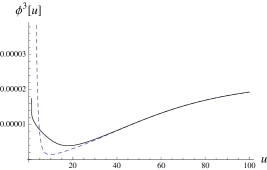
Figure 9: Comparison of analytical (dashed) and numerical solutions for $u<100$. The agreement is good for large $u$ as expected.

Figure 10: Comparison of analytical (dashed) and numerical solutions for asymptotic values of $u$. The dashed line is not visible as the agreement is good.

A technical comment about the numerical solutions is that equation (4.10) is not automatically implemented. However gauge invariance of the action implies the following relation between the equations: $D_{\mu}{\partial\cal L\over\partial A_{\mu}}+ie[\phi,{\partial\cal L\over\partial\phi}]=0\;$. Thus, in this context it means that

$$\partial_{u}({\partial S\over\partial A_{u}^{-}})=2iA_{u}^{+}({\partial S\over\partial A_{u}^{3}})+iA_{0}^{3}({\partial S\over\partial A_{0}^{-}})+i(\phi_{3}({\partial S\over\partial\phi^{-}})-2\phi^{+}({\partial S\over\partial\phi^{3}}))$$ (4.14)

This means that if the other equations are satisfied (4.10) must evaluate to a constant. Thus for some choice of boundary conditions this constant will become zero and the equation will be satisfied. Thus we have scanned over different values of the boundary values till (4.10) evaluates to zero. The result of this is an exact solution that satisfies all the equations of motion. This is shown in Figures 5,6,7 and 8. The value of the $SU(2)$ fields for this solution are very small in the entire region and hence the Yang-Mills approximation to DBI is reliable. This then establishes unambiguously that a condensate is indeed formed.

5 Phases as a function of $\mu$ and $T$

This section summarizes the phase structure (at zero temperature) based on the calculations of the earlier sections. To study the thermodynamics we go to Euclidean section by setting $it=t_{E}$ where $t_{E}$ has a period $\beta={1\over T}\;$. To compare the phases at zero temperature we consider the Euclidean action with $\beta=\infty$, which effectively means consider the coefficient of $\beta$. We have a background field $A_{0}=A_{t}$. Wick rotation converts this to $A_{t_{E}}$ which satisfies $A_{t_{E}}dt_{E}=A_{t}dt$. Thus $A_{t_{E}}={A_{t}\over i}\;$. When one does the Euclidean functional integral we analytically continue to real $A_{t_{E}}$ and integrate over real $A_{t_{E}}$ field configurations. However if there is a background real $A_{t}$ (that is a solution of the classical Minkowski equations with a real charge), this has to be put in as an imaginary background value for $A_{t_{E}}\;$. Thus if one wants to perform the functional integral at one loop, then one has to work with real $A_{t_{E}}$ fluctuating about an imaginary background value. However at the classical level, we need not do all this - we can just plug in the Minkowski solution into the action without introducing $A_{t_{E}}\;$.

Since the configurations depend only on $u$, we need only worry about the $u$ integral. Thus we need to look at $S[A^{3}_{0}(u),\;\tau(u)]$ evaluated on the solutions.

As a first step we just consider the solutions of the Dirac-Born-Infeld equations considered in Section 1 where the sources are localized as $\delta(u-u_{c})$. This can tell us whether the phase with $t_{3}$ number being non zero is preferred over the phase with net $t_{3}$ number being zero. We remind the reader that we are referring to the $t_{3}$ component of the $U(1)\times SU(2)\;$. ($t_{a}\;$ are the $SU(2)$ generators.) We assume that the $U(1)_{B}$ baryon charge is already non zero and we have the cusp configuration. When $t_{3}$ number is non zero, one can further ask whether there is a $t_{3}$ number violating condensate. This has to be asked within the Yang-Mills approximation. This is the second step.

The Dirac-Born Infeld action with source is (see equation (2.4))

$$S_{DBI}=-\tilde{T}\int~{}d\sigma~{}{u^{5\over 2}\over\sqrt{f}}\;\;[u^{\prime 2}+u^{3}f^{2}\tau^{\prime 2}-f(\partial_{\sigma}a_{0})^{2}]^{1\over 2}-n_{B}\tilde{T}a_{0}(u_{c})$$ (5.1)

and the solution for $a_{0}$ is

$$(\partial_{u}a_{0})^{2}={d_{0}^{2}\;(1+u^{3}f^{2}{\tau^{\prime}}^{2})\over f\;(u^{5}+d_{0}^{2})}$$ (5.2)

This determines $a_{0}(u)$ in terms of $d_{0}$. In our case we have two branes. We write $d_{1},d_{2}$ corresponding to the two branes as:

$$d_{1}=d_{0}+{d_{3}\over 2}~{}~{}~{}~{}d_{2}=d_{0}-{d_{3}\over 2}$$

where $d_{3}$ is the $t_{3}$ charge that we are concerned with. The chemical potential $\mu_{3}=A^{3}_{0}(\infty)$. We will fix a gauge by setting $A^{3}_{0}(u_{c})=0\;$.

We have two branes with different profiles $\tau(u)$, which in turn depend on the constants $d$ and $c$, see equation (2.10) . We need to impose that $u_{c}$ is the same for both branes. So if $d_{1},c_{1}$ are given, then $u_{c}$ is fixed and so $c_{2}$ is fixed once $d_{2}$ is. Thus we Legendre transform $\tau^{\prime}(u)$ in terms of $c_{0}$. We can also substitute the solution for $a_{0}(u)$ and $\tau(u)$. Thus we find that the Legendre transformed (with respect to $\tau$) is

$$\Omega(\mu,\;c_{0})={fu^{8}-c_{0}^{2}\over fu^{3\over 2}\;\sqrt{D(d_{0},c_{0})}}\;\;\;,\;\;\;\;D(d_{0},c_{0})=u^{8}f+d_{0}^{2}u^{3}f-c_{0}^{2}\;\;.$$

Generalizing to two branes one finds:

$$\Omega(\mu_{0},\mu_{3},c_{0})=\int du\;\left({fu^{8}-c_{1}^{2}\over fu^{3\over 2}\;\sqrt{D(d_{1},c_{1})}}+{fu^{8}-c_{2}^{2}\over fu^{3\over 2}\;\sqrt{D(d_{2},c_{2})}}\right)$$

where $d_{1}=d_{0}+{d_{3}\over 2}$ and $d_{2}=d_{0}-{d_{3}\over 2}\;$.

One can compare this action with the action with $d_{3}=0$ and the same value of $\mu_{3}$ at the boundary. If $d_{3}=0$ then the branes are right on top of each other and there is no separation. Thus not only is there no $t_{3}$ charge, there is also no $t_{3}$ number violating condensate. We have an unbroken $SU(2)$ gauge symmetry. If $d_{3}=0$ then $A^{3}_{0}$ is constant everywhere and is pure gauge. The action is

$$\Omega_{0}(\mu_{0},\mu_{3},c_{0})=2\;\int du\;{fu^{8}-c_{0}^{2}\over fu^{3\over 2}\;\sqrt{D(d_{0},c_{0})}}\;\;.$$

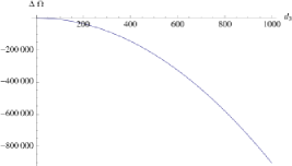
Figure 11: Free Energy difference: $c_{1}=10^{3},d_{1}=10^{3}$

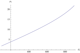
Figure 12: $\mu_{3}$ vs $d_{3}$ with $c_{1}=10^{3},d_{1}=10^{3}$

The precise relation between $\mu$ and $d_{0}$ can be obtained by first calculating the free energy $F(d_{0},c_{0})$ with fixed $d_{0}$ (Legendre transform of $\Omega$ with respect to $\mu\;$, or equivalently, of $S$ with respect to $a_{0}\;$).

$$F(d_{0},c_{0})=\tilde{T}\;\int_{u_{c}}^{\infty}du\;{\sqrt{D(d_{0},c_{0})}\over f(u)u^{3\over 2}}\;\;+\;{\tilde{T}\;d_{0}\over 3}\;u_{c}\;\;.$$

We have included the D4-brane action of the $U(1)$ charges. This gives

$$\mu={\partial F\over\partial d_{0}}=\tilde{T}\int_{u_{c}}^{\infty}du~{}\partial_{u}a_{0}\;+\;{\tilde{T}\;u_{c}\over 3}=\tilde{T}\int_{u_{c}}^{\infty}du~{}{d_{0}u^{3\over 2}\over\sqrt{D(d_{0},c_{0})}}\;+\;{\tilde{T}\;u_{c}\over 3}\;\;.$$

The free energy difference is $\Omega(d_{1})+\Omega(d_{2})-2\;\Omega(d_{0})\;$. This has to be plotted for different $\mu_{3}$ keeping fixed $\mu_{0}=\mu_{1}+\mu_{2}$. It is simpler to plot the free energy $\Omega$ as a function of $d_{3}$ and give a separate plot giving $\mu_{3}$ versus $d_{3}$.

The chemical potential is given by:

$$\mu_{3}=\mu_{1}-\mu_{2}=\int_{u_{c}}^{\infty}du~{}\left({d_{1}u^{3\over 2}\over\sqrt{D(d_{1},c_{1})}}\;-\;{d_{2}u^{3\over 2}\over\sqrt{D(d_{2},c_{2})}}\right)$$

Figure 12 shows a plot of $\mu_{3}$ vs $d_{3}$ for the separated D8 brane solution (i.e. with a $t_{3}$ number) for a sample value of $c_{0},d_{0}\;$. The free energies are plotted as a function of $d_{3}$ in Figure 11. We see that for all values of $d_{3}$ the free energy difference is negative. For e.g. for $d_{3}=10$ (so that $d_{3}<<d_{0}$), we find that $\Delta\Omega\simeq-89.97\;$. Thus one infers that as $\mu_{3}$ increases so does $d_{3}$ (see Figure 12), and so (see Figure 11) one has a phase transition to the phase with non zero $t_{3}$ number.

We have thus established that when there is a non zero chemical potential for $t_{3}$ the phase with a finite number density of $t_{3}$ charge is favored. We also have exact (numerical) solutions for this phase which have charged fields condensing. A calculation of the free energy difference for the given exact solution gives $\simeq-4.40*10^{-4}$ and shows that this condensate is favored over the trivial solution (with condensate being zero). Thus putting these results together we have established that a BCS condensate is formed and we have a holographic description of the ground state. This is the main conclusion of this paper. We now discuss below the implications of this for the boundary theory.

Our experience with the boundary BCS theory says that there should be a condensate, since when there is a finite number density of fermions, and hence a Fermi Surface, one expects the BCS instability. This should thus reflect itself in a $t_{3}$ number violating condensate of charged fields. As mentioned above the existence of this condensate is proved by the holographic calculation.

The nature of the boundary condensate also needs to be determined. As discussed in the Introduction the most plausible candidate seems to be a BCS like Cooper pair $BB$ if $N_{c}$ is odd. We are at zero temperature and in the confining phase in the boundary. $B=\epsilon_{a_{1},a_{2},\cdots,a_{N_{c}}}u^{a_{1}}d^{a_{2}}u^{a_{3}}d^{a_{4}}\cdots u^{a_{N_{c}}}$. If $N_{c}$ is even, one could have scalar baryons with $t_{3}=+1$ condensate. This would be analogous to a BEC because the particles are strongly bound already, before they condense.

The effect of this condensate should be visible in the conductivity. Thus if one calculates the current current correlator one should find a gap in the imaginary part (equivalently in the real part of the conductivity). This is a problem for the future. In the next section we take a first step in this direction by considering the conductivity of the Sakai-Sugimoto model without any $SU(2)$ breaking.

6 Conductivity

Consider the DBI action given by equation (2.4) with $n_{B}=0$ and $\sigma=u\;$,

$$S_{DBI}=-\tilde{T}\int d^{4}x~{}du~{}{u^{5\over 2}\over\sqrt{f}}\;\;[1+u^{3}f^{2}\tau^{\prime 2}-f(\partial_{u}a_{0})^{2}]^{1\over 2}\;\;.$$ (6.1)

The equations of motion are

$$\frac{u^{11}f^{3}\;\tau^{\prime 2}}{1+u^{3}f^{2}\tau^{\prime 2}-f(\partial_{u}a_{0})^{2}} = c_{0}^{2}$$

$$\frac{u^{5}f\;(\partial_{u}a_{0})^{2}}{1+u^{3}f^{2}\tau^{\prime 2}-f(\partial_{u}a_{0})^{2}} = d_{0}^{2}$$ (6.2)

where $c_{0}$ and $d_{0}$ are constants. These equations imply, see equations (2.10),

$$(\partial_{u}a_{0})^{2}={d_{0}^{2}\;u^{3}\over D}\;\;\;,\;\;\;\;(\partial_{u}\tau)^{2}={c_{0}^{2}\over u^{3}f^{2}D}$$ (6.3)

where $D=u^{8}f+d_{0}^{2}u^{3}f-c_{0}^{2}\;$ and, hence, that

$${\cal L}={u^{5\over 2}\over\sqrt{f}}\;\;[1+u^{3}f^{2}\tau^{\prime 2}-f(\partial_{u}a_{0})^{2}]^{1\over 2}=\frac{u^{13\over 2}}{\sqrt{D}}\;\;.$$ (6.4)

The $D8$ brane ends at $u=u_{0}$ where $\partial_{u}\tau\to\infty$ i. e. $D(u_{0})=0\;$. This gives $u_{0}$ in terms of other parameters as

$$(u_{0}^{5}+d_{0}^{2})\;u_{0}^{3}f_{0}=c_{0}^{2}\;\;,\;\;\;f_{0}=f(u_{0})\;\;.$$ (6.5)

6.1 Fluctuation about the background

Let us turn on the $U(1)$ gauge field $a_{2}(\sigma^{\mu})$ along the $\sigma^{2}=x\;$ direction of the $D8$ brane worldvolume. We will consider this as small fluctuation around the background described in previous section and neglect any back reaction. For simplicity let us first assume $a_{2}$ to be a function of $t$ and $u$ only. We will also assume $a_{2}(t,u)=a(u)e^{-i\omega t}$. Let a dot $(\dot{})$ and a prime (^′) denote $t$ and $u$ derivatives.

For matrices $M$ and $\delta M$, where $\delta M$ is assumed to be small, we have

$$\frac{\sqrt{det\;(M+\delta M)}}{\sqrt{det\;M}} = 1+\frac{1}{2}\;tr(M^{-1}\delta M)+\frac{1}{8}\;\left(tr(M^{-1}\delta M)\right)^{2}$$ (6.6)

$$-\frac{1}{4}\;tr(M^{-1}\delta M)^{2}+{\cal O}(\delta M)^{3}\;\;.$$

Applying this relation to the Lagrangian ${\cal L}_{DBI}=\sqrt{det\;(G+F+\delta F)}\;$ gives

$${\cal L}_{DBI}\approx\mathcal{L}-\frac{1}{4}\mathcal{L}~{}~{}tr((G+F)^{-1}\delta F)^{2}+{\cal O}(\delta F)^{3}$$ (6.7)

where ${\cal L}=\sqrt{det\;(G+F)}\;$. For the problem considered here, ${\cal L}$ is given explicitly in equation (6.4), and we have $\;tr((G+F)^{-1}\delta F)=0\;$. We can construct $3\times 3$ matrices out of $(G+F)$ and $\delta F$ to compute the traces, as $\delta F$ is of the form,

$$\delta F=\left(\begin{array}[]{cccc}0&0&\dot{a}_{2}&\\ 0&0&a_{2}^{\prime}&\mbox{\Huge$0$}\\ -\dot{a}_{2}&-a_{2}^{\prime}&0&\\ &\mbox{\Huge$0$}&&\\ &&&\mbox{\Huge$0$}\end{array}\right)\;\;.$$ (6.8)

Let us call the truncated blocks of $(G+F)$ and $\delta F\;$ as $B$ and $\delta B$ respectively,

$$B = \left(\begin{array}[]{ccc}-u^{3\over 2}&-a_{0}^{\prime}&0\\ a_{0}^{\prime}&\frac{1}{u^{3\over 2}f}(1+u^{3}f^{2}\tau^{\prime}(u)^{2})&0\\ 0&0&u^{3\over 2}\end{array}\right)$$ (6.12)

$$\delta B = \left(\begin{array}[]{ccc}0&0&\dot{a}_{2}\\ 0&0&a_{2}^{\prime}\\ -\dot{a}_{2}&-a_{2}^{\prime}&0\end{array}\right)$$ (6.16)

Then,

$$tr((G+F)^{-1}\delta F)^{2}=\frac{1}{\mathcal{L}^{2}}\;\frac{2u^{2}}{f}\;((1+u^{3}f^{2}\tau^{\prime 2})(\dot{a}_{2})^{2}-u^{3}f(a^{\prime}_{2})^{2})$$ (6.17)

Then the Lagrangian $\mathcal{L}_{f}$ for the fluctuations is given by

$$\mathcal{L}_{f}=\frac{1}{2}\left(\frac{(u^{5}+d_{0}^{2})}{\sqrt{u^{3}D}}\;(\dot{a}_{2})^{2}-\sqrt{D\over u^{3}}\;(a^{\prime}_{2})^{2}\right)\;\;.$$ (6.18)

The equation of motion is then given by

$$\left(\sqrt{D\over u^{3}}\;a^{\prime}_{2}\right)^{\prime}-\frac{(u^{5}+d_{0}^{2})}{\sqrt{u^{3}D}}\;\ddot{a}_{2}=0\;\;.$$ (6.19)

Setting $a_{2}(t,u)=a(u)e^{-i\omega t}$, we get

$$\left(\sqrt{D\over u^{3}}\;a^{\prime}\right)^{\prime}+\frac{(u^{5}+d_{0}^{2})}{\sqrt{u^{3}D}}\;\omega^{2}=0\;\;.$$ (6.20)

The equation of motion is same for the world volume fluctuations considered above for both $D8$ and $\overline{D8}$ branes. In the absence of charges, continuity of flux would require that the fields continue in the same direction along the other brane and reemerge on the boundary. So we can consider $a(u)$ to be the field on both $D8$ and $\overline{D8}$ branes, but $u$ is a bad co-ordinate choice for such a representation. We can consider a change of co-ordinate given by $y^{2}=1-\frac{u_{0}}{u}$. $y\in(0,1)$ corresponds to brane and $y\in(0,-1)$ anti-brane. The brane and anti-brane are joined at $y=0\;$, the $y=\pm 1$ are corresponds to the intersection of the brane and anti brane with $D4\;$. We will call $y=1$ boundary and $y=-1$ the “horizon”. The differential equation will be solved with “in-going boundary condition at the horizon”, and we will use “AdS/CFT correspondence” to evaluate the boundary Green’s function.

This choice of boundary condition does not have a rigorous justification. However we can argue heuristically. We want boundary conditions corresponding to the normal modes or more correctly quasi normal modes. The eigenvalues then give the poles of the Green function. We motivate boundary conditions as follows. In the case of the black hole, in the AdS/CFT context, these boundary conditions were first introduced in [48, 49] where it was argued that at the horizon, ingoing boundary conditions are useful because with the usual Dirichlet/Neumann boundary condition the eigenvalues are strictly real. The latter would give real poles for the boundary Green function and would not describe thermalization which requires an imaginary part for the poles. Ingoing boundary condition is one option that does give an imaginary part to the pole location. Furthermore ingoing boundary condition has the reasonable physical interpretation of complete absorption by the black hole.

In the present case also we only have a few reasonable boundary conditions and we pick one that seems to give the right pole structure. Ingoing, is one such and corresponds to perfect absorption. Are there situations other than a black hole horizon where one expects complete absorption? The answer is yes. Consider electromagnetic waves in a wave guide with an oscillator source at one end and the other end open and radiating via an antenna into three dimensional space. The cross section of the wave guide is two dimensional. It is well known that when there is impedance matching the entire output of the wave guide is radiated and there is no reflection at the boundary. The radiating antenna behaves like a perfect absorber at the end of the wave guide. The correct boundary condition inside the wave guide in such a situation is the ingoing one. Thus perfect absorption is not unknown outside the black hole context. In our case we have a lower dimensional wave propagation channel opening out into a higher dimensional space - the cross section of the D8 brane is effectively three dimensional and is connecting to a four dimensional D4 brane. This gives a possible physical motivation for considering ingoing boundary conditions in the present situation.

We will set $u_{KK}=1$ in all the future calculations. The differential equation for $a(y)$ near “horizon”, i.e. near $y=-1\;$, is given by

$$(1+y)\;\frac{d^{2}a}{dy^{2}}-\frac{1}{2}\;\frac{da}{dy}+\frac{2\omega^{2}}{u_{0}}a=0$$ (6.21)

which gives the near-horizon behavior of $a(y)$ as,

$$a\sim e^{\pm i\frac{2\sqrt{2}\omega}{\sqrt{u_{0}}}\sqrt{1+y}}$$ (6.22)

The solution $a\sim e^{-i\frac{2\sqrt{2}\omega}{\sqrt{u_{0}}}\sqrt{1+y}}$ gives the in-going wave. Let $a(y)=e^{-i\frac{2\sqrt{2}\omega}{\sqrt{u_{0}}}\sqrt{1+y}}\rho(y)\;$. Then the differential equation for $\rho(y)$ is solved numerically to obtain $a(y)$, with boundary condition that $\rho(y_{h})=1+\frac{2\sqrt{2}i\omega}{\sqrt{u_{0}}}\sqrt{1+y_{h}}$ and $\rho^{\prime}(y_{h})=\frac{\sqrt{2}~{}i~{}\omega}{\sqrt{u_{0}}\sqrt{1+y_{h}}}\;$, where $y_{h}$ is a cut-off near $y=-1\;$. The expression for $\rho(y_{h})$ is obtained by doing a series solution of the differential equation near $y=-1\;$.

The differential equation for $a(y)$ near “boundary”, i.e. near $y=+1\;$, is given by

$$(1-y)\;\frac{d^{2}a}{dy^{2}}+\frac{1}{2}\;\frac{da}{dy}+\frac{2\omega^{2}}{u_{0}}a=0$$ (6.23)

The solution for $a(y)$ near boundary, i.e. near $y=+1\;$, behaves as

$$a(y) \sim A\;(1+A_{1}(1-y)+A_{2}(1-y)^{2}+\cdots)$$ (6.24)

$$+B\;(1-y)^{\frac{3}{2}}\;(1+B_{1}(1-y)+B_{2}(1-y)^{2}+\cdots)$$

where $A$ and $B$ are arbitrary constants determined by boundary conditions. $A_{i}$ and $B_{i}$ are constants determined in terms of parameters of the differential equation. So, the Green’s function is given by,

$$G_{R}(\omega,u_{0},d_{0})\sim\frac{B}{A}=\lim_{y\to 1}\;\frac{\frac{4}{3}~{}\sqrt{(1-y)}}{a(y)}\;\frac{d^{2}a}{dy^{2}}\;\;.$$ (6.25)

The conductivity can then be obtained by

$$\sigma=\frac{G_{R}}{i~{}\omega}\;\;.$$ (6.26)

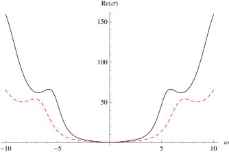
Figure 13: Real part of Conductivity with $d_{0}=0$: $u_{0}=10$ (Black, continuous) and $u_{0}=15$ (Red, dashed)

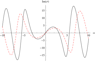
Figure 14: Imaginary part of Conductivity with $d_{0}=0$: $u_{0}=10$ (Black, continuous) and $u_{0}=15$ (Red, dashed).

Figures 13 and 14 show variation of conductivity with frequency. We have set $d_{0}=0$ in our conductivity calculations as the variation of conductivity with $d_{0}$ is very small.

6.2 Modified Sakai-Sugimoto model

In the original paper, the scalar bi-fundamental tachyon field arising from open string between $D8$ and $\overline{D8}$-brane was neglected. Later various authors [27, 34] have included the contribution of the tachyon field which is expected to be the origin of quark mass and condensate. The effect of tachyon field for the case of gauge field fluctuation is that the fluctuations become massive, with mass proportional to the tachyon field. The tachyon field has an approximate behavior like $e^{-\frac{u}{u_{0}}}$ asymptotically. We will assume the mass term corresponding to the $a_{2}$ fluctuation is proportional to $m_{0}^{2}e^{-\frac{u}{u_{0}}}\;$, to get a qualitative nature of the effect of tachyon on the conductivity. More rigorous analysis needs to be done for quantitative results. Let us consider the modification of equation (6.20) given by

$$\left(\sqrt{D\over u^{3}}\;a^{\prime}\right)^{\prime}+\frac{(u^{5}+d_{0}^{2})}{\sqrt{u^{3}D}}\;(\omega^{2}-m_{0}^{2}e^{-\frac{u}{u_{0}}})=0\;\;.$$ (6.27)

A similar analysis, as in the previous section, can be done to obtain conductivity. Figures 15 and 16 show the conductivity for various values of $m_{0}\;$. We see that with a non-zero value of $m_{0}$ the conductivity develops a mass-gap. Effect of $d_{0}$ on the conductivity is very small, and we have set $d_{0}=0$ for all our numerics. As we increase $m_{0}$, both mass gap and peak heights increases. Also, for any finite value of $m_{0}$, a pole appears at $\omega=0$ for the imaginary part of conductivity (fig. 16), which implies a delta function peak for real part of the conductivity by Kramers-Kronig relation. The delta function function peak can not be captured by numerics.

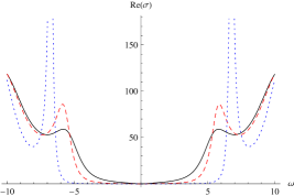
Figure 15: Real part of Conductivity with $d_{0}=0$, $u_{0}=10$: $m_{0}=0$ (Black, continuous), $m_{0}=5$ (Red, dashed) and $m_{0}=10$ (Blue, dotted). As we increase the mass $m_{0}$, the peak height increases. The peak for $m_{0}=10$ is outside the range of the ordinate value shown in the figure.

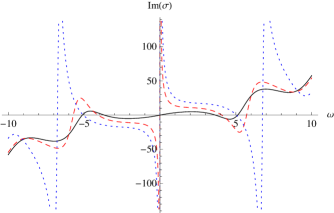
Figure 16: Imaginary part of Conductivity with $d_{0}=0$, $u_{0}=10$: $m_{0}=0$ (Black, continuous), $m_{0}=5$ (Red, dashed) and $m_{0}=10$ (Blue, dotted). The peak for $m_{0}=10$ is outside the range of the ordinate value shown in the figure

7 Summary and Conclusions

In this paper we have attempted to find a holographic description of the BCS Cooper pairing instability and thence describe the strong coupling microscopic BCS phenomenon. The analogy with chiral symmetry breaking in QCD was exploited and the Sakai Sugimoto model with finite number density of flavored fermions was studied. The background charge corresponds to a $U(1)_{3}$ embedded in the $SU(2)_{flavour}$. The flavor $SU(2)$ was broken to $U(1)_{3}$ by the background and it was shown that in this situation there is a tachyonic instability that causes fields charged under this $U(1)_{3}$ to condense. This is the bulk description of the BCS instability. Analytic solutions describing this condensate were given in flat space. The stability properties were also studied. The curved space equations were then solved analytically in some approximation. The exact solutions have also been done numerically. The free energy difference shows that this solution is favored over the trivial solution. This solution then describes the BCS ground state of the superconductor.

Once we have this solution one should be able to calculate various quantities such as the AC conductivity using the AdS/CFT dictionary. However there are two complications. One is that the bulk is not asymptotically AdS. The second is that the flavor branes do not extend all the way to the interior. Thus the usual “infalling” boundary conditions prescription has to be modified. A preliminary exploration of this problem in the original Sakai-Sugimoto model was done in Section 7. The chiral current Greens function was calculated. It has the expected properties of a mass gap.

The detailed analysis of this in the context of the Sakai-Sugimoto model as well as in the modified form in this paper need to be studied. Another important question is to look for the bulk signature of the Fermi surface in the boundary.

We hope to return to these questions soon.

Acknowledgements: We thank G. Baskaran and R. Shankar for many useful discussions. We also thank the unknown referee of Nuclear Physics B for very useful comments.

Appendix A $D8$ brane with non zero electric field

In this Appendix, we formulate the equations describing the profile of $D8$ brane in the background of $D4$ branes, and with a non zero world volume electric field turned on.

We write the Dirac-Born-Infeld part of the $D8$ brane action in the ten dimensional background of $D4$ branes as

$$S_{DBI}=-C_{9}\;\int d^{9}\sigma\;g_{s}e^{-\Phi}\;\sqrt{-det\;G}$$

where the components $G_{\mu\nu}$ of the matrix $G$ are given by

$$G_{\mu\nu}=g_{MN}\;\partial_{\mu}X^{M}\partial_{\nu}X^{N}+F_{\mu\nu}$$

with $g_{MN}$ being the ten dimensional background metric,

$$X^{M}=(x^{0},u,x^{1},x^{2},x^{3},\tau,\theta^{1},\cdots,\theta^{4})$$

are the ten dimensional coordinates with $\tau\sim\tau+2\pi r_{4}$, and $F_{\mu\nu}=\partial_{\mu}a_{\nu}-\partial_{\nu}a_{\mu}$ is the $U(1)$ gauge field strength on the brane. We choose the nine dimensional brane coordinates $\sigma^{\mu}$ to be given by

$$\sigma^{\mu}=(x^{0},\sigma,x^{1},x^{2},x^{3},\theta^{1},\cdots,\theta^{4})\;\;.$$

We consider the case where $a_{0}$ is the only non vanishing component of the $U(1)$ gauge field and $(u,\tau,a_{0})$ depend on $\sigma$ only. The functions $u(\sigma)$ and $\tau(\sigma)$ describe the $D8$ brane profile in the $(u,\tau)$ plane. It then follows that

$$G_{\sigma\sigma}=g_{uu}\;u_{\sigma}^{2}+g_{\tau\tau}\;\tau_{\sigma}^{2}\;\;\;,\;\;\;G_{0\sigma}=-G_{\sigma 0}=F_{0\sigma}=-(a_{0})_{\sigma}\;\;,$$

and $G_{\mu\nu}=g_{\mu\nu}$ otherwise. The subscripts $\sigma$ on $(u,\tau,a_{0})$ denote their
$\sigma-$derivatives.

In order to solve the equations of motion which follow from the action $S_{DBI}$ and to obtain the $\sigma-$dependence of $(u,\tau,a_{0})$, note that $S_{DBI}$ now resembles a world line action

$$S_{DBI}\sim\;\int d\sigma\;\sqrt{h_{\alpha\beta}\;\xi^{\alpha}_{\sigma}\xi^{\beta}_{\sigma}}$$

where $\xi^{\alpha}=(u,\tau,a_{0})$, the subscript $\sigma$ on $\xi$ denotes its $\sigma-$derivative. For our case, $g_{MN}$ is diagonal and we have $h_{\alpha\beta}\equiv diag\;(h_{1},h_{2},h_{3})\;$ where

$$h_{1} = g_{s}^{2}e^{-2\Phi}\;(-\;det\;g_{\mu\nu})\;|_{\sigma=u}$$

$$h_{2} = g^{uu}g_{\tau\tau}\;h_{1}$$

$$h_{3} = g^{uu}g^{00}\;h_{1}$$

and depend on $\xi^{1}=u$ only. The consequent ‘geodesic’ equations then give

$$h_{2}\;\tau_{\sigma}=c_{0}$$ (A.1)

$$h_{3}\;(a_{0})_{\sigma}=d_{0}$$ (A.2)

$$h_{1}\;u_{\sigma}^{2}+h_{2}\;\tau_{\sigma}^{2}+h_{3}\;(a_{0})_{\sigma}^{2}=E$$ (A.3)

$$2\;h_{1}\;u_{\sigma\sigma}+(h_{1})_{u}\;u_{\sigma}^{2}-(h_{2})_{u}\;\tau_{\sigma}^{2}-(h_{3})_{u}\;(a_{0})_{\sigma}^{2}=0$$ (A.4)

where $c_{0}$, $d_{0}$, and $E$ are constants and the subscripts $u$ on the $h$s denote their $u-$derivatives. It follows from the above equations that

$$u_{\sigma}^{2}=\frac{1}{h_{1}}\;\left(E-\frac{c_{0}^{2}}{h_{2}}-\frac{d_{0}^{2}}{h_{3}}\right)\;\;.$$ (A.5)

The right hand side of the above equation is a function of $u\;$. Generically the location $u=u_{0}$ of its zero, if exists, denotes a turning point for $u(\sigma)$. Thus if $u(\sigma)\to u_{0}$ from above as $\sigma\to\sigma_{0}$ then, generically, $u$ starts increasing as $\sigma$ increases beyond $\sigma_{0}\;$ which can be seen from $u_{\sigma\sigma}$ equation. Also, generically, the evolution of $\tau(\sigma)$ and $a_{0}(\sigma)$ is monotonous across $\sigma_{0}\;$. In the context of $D8$ branes in the background of $D4$ branes, $u_{0}$ will denote the lowest point of $D8$ brane profile in the $(u,\tau)$ plane. Also, $(a_{0})_{\sigma}$ equation above with $d_{0}\neq 0$ shows that such a $D8$ brane can support a non trivial $U(1)$ gauge field on its worldvolume. It is now straightforward to obtain the evolution in terms of $u$ alone using $\tau_{u}=\frac{\tau_{\sigma}}{u_{\sigma}}$ and similarly for $(a_{0})_{u}\;$. Using $F_{0u}=-(a_{0})_{u}\;$ and the expressions for $h_{2}$ and $h_{3}\;$ in equation (A.3), we have

$$\Delta\equiv 1+g^{uu}g_{\tau\tau}\;\tau_{u}^{2}+g^{00}g^{uu}\;F_{0u}^{2}=\frac{E}{h_{1}\;u_{\sigma}^{2}}$$ (A.6)

where $u_{\sigma}^{2}$ is given in equation (A.5).

Writing the ten dimensional background fields of $D4$ branes as

$$ds_{10}^{2} = g_{MN}dx^{M}dx^{N}$$

$$= H^{-\frac{1}{2}}\left(-(dx^{0})^{2}+\sum_{i=1}^{3}(dx^{i})^{2}+fd\tau^{2}\right)+H^{\frac{1}{2}}\left(\frac{du^{2}}{f}+u^{2}d\Omega_{4}^{2}\right)$$

and $e^{\Phi}=g_{s}\;H^{-\frac{1}{4}}\;$ where $H=\frac{1}{u^{3}}\;$, and $f=1-\frac{u_{KK}^{3}}{u^{3}}\;$, we have

$$(h_{1},h_{2},h_{3})=u^{8}\;\left(\frac{H}{f},\;f,\;-H\right)\;\;,\;\;\;u_{\sigma}^{2}=\frac{D}{Hu^{16}}\;\;,\;\;\;\Delta=\frac{u^{8}f\;E}{D}$$

where $D=(Eu^{8}+\frac{d_{0}^{2}}{H})f-c_{0}^{2}\;$, and

$$(a_{0})_{u}^{2}=\frac{d_{0}^{2}}{H\;D}\;\;,\;\;\;\;\tau_{u}^{2}=\frac{c_{0}^{2}\;H}{f^{2}\;D}\;\;.$$

The expressions for $(a_{0})_{u}^{2}\;$ and $\tau_{u}^{2}$ given in equations (2.10) correspond to the choice $E=1\;$.

Appendix B Embedding of the $SU(2)$ group in $SU(2N_{d})$

We have two sets of coincident branes. For concreteness and clarity of presentation let us assume that each coincident set has three branes, i.e $N_{d}=3$. (The minimum required is two). So we have six branes in all. Our configuration breaks $U(1)\times SU(6)$ down to $U(1)\times U(1)\times SU(3)\times SU(3)$. We have 36 generators in $U(6)$. We can write them using the direct product notation. Let $\lambda$ stand for the Gell-Mann Lambda matrices for the $SU(3)$ part: $\lambda^{1,2,..8}$ and $\lambda^{0}$ be the identity matrix.

$$\lambda^{0}=\left(\begin{array}[]{ccc}1&0&0\\ 0&1&0\\ 0&0&1\end{array}\right)$$

Similarly $\sigma^{1,2,3}$ are the $SU(2)$ matrices with $\sigma^{0}$ being the identity.

Then the unbroken generators of $U(6)$ are: $\lambda^{0}\otimes\sigma^{0},\lambda^{0}\otimes\sigma^{3}$ are the two unbroken $U(1)$’s. Schematically (the labels 1,2 stand for the two branes):

$$U(1)_{1}=\left(\begin{array}[]{cc}\lambda^{0}&0\\ 0&0\end{array}\right);~{}~{}~{}U(1)_{2}=\left(\begin{array}[]{cc}0&0\\ 0&\lambda^{0}\end{array}\right)$$

or equivalently:

$$U(1)_{B}=\left(\begin{array}[]{cc}\lambda^{0}&0\\ 0&\lambda^{0}\end{array}\right);~{}~{}~{}U(1)_{3}:2t_{3}=\left(\begin{array}[]{cc}\lambda^{0}&0\\ 0&-\lambda^{0}\end{array}\right)$$ (B.1)

Similarly $\lambda^{a}\otimes(\sigma^{0}+\sigma^{3})/2,\lambda^{a}\otimes(\sigma^{0}-\sigma^{3})/2,~{}~{}a~{}=1,2...8$ are the two $SU(3)$. These are not excited in our condensate solutions. They do contribute in an instanton contribution localized at $u=u_{c}$. They generate the Chern Simons interaction which gives a source at $u=u_{c}$. Schematically:

$$\left(\begin{array}[]{cc}\lambda^{a}&0\\ 0&0\end{array}\right);~{}~{}~{}\left(\begin{array}[]{cc}0&0\\ 0&-\lambda^{a}\end{array}\right)$$ (B.2)

The eighteen broken generators are:

$\lambda^{0}\otimes\sigma^{1,2}$ are the generators corresponding to the $W^{1,2}$ massive gauge fields of the $SU(2)$ that condense. Schematically

$$t_{1}=\left(\begin{array}[]{cc}0&\lambda^{0}\\ \lambda^{0}&0\end{array}\right);~{}~{}~{}t_{2}=\left(\begin{array}[]{cc}0&-i\lambda^{0}\\ i\lambda^{0}&0\end{array}\right)$$ (B.3)

Finally the sixteen $\lambda^{a}\otimes\sigma^{1,2}$ are the broken generators corresponding to gauge fields that are not excited. Schematically:

$$\left(\begin{array}[]{cc}0&\lambda^{a}\\ \lambda^{a}&0\end{array}\right);~{}~{}~{}\left(\begin{array}[]{cc}0&-i\lambda^{a}\\ i\lambda^{a}&0\end{array}\right)$$ (B.4)

The total number of generators is 36 as required for $U(6)$. This is easily generalized to $U(2N_{d})$.

The Yang-Mills analysis in this paper involves $t_{1},t_{2},t_{3}$. As can be seen they see nothing of the $SU(3)$ internal structure. Hence these indices are suppressed in all the equations of this paper.

Thus for each set of three coincident D8 branes the DBI analysis given in this paper follows that of [20, 34].

Appendix C Symmetrized Trace Prescription

In this appendix we give a useful result on symmetrized trace (Str) prescription. This is useful in the two flavor case when there is only the $0$ component of the $U(2)$ Yang-Mills fields being non-zero and the branes are on top of each other (so that the symmetric “metric” part of the Dirac-Born-Infeld is proportional to the identity). Evaluate using symmetrized trace prescription the object

$$e^{{1\over 2}\;Tr\;ln(1+F_{3}+F)}\;\;.$$

The prescription is to expand in a power series in $F_{3}+F$ and symmetrize each term.

Let $F=F^{+}\tau^{+}+F^{-}\tau^{-}$ and $F_{3}={1\over 2}\;F^{3}\tau^{3}\;$.

Observations:

1. Since $F_{u0}=-F_{0u}$ is the only non zero component, the trace (over Lorentz indices) of an odd number of $F$’s is zero.

2. $$F_{3}^{2}={(F^{3})^{2}\over 4}I$$

   $$F^{2}=F^{+}F^{-}\{\tau^{+},\tau^{-}\}=F^{+}F^{-}I$$

   $$F_{3}F+FF_{3}=0\;\;.$$

3. Consider a term $F_{3}^{n}F^{m}$. It has to be symmetrized completely so we have all permutations. Consider the first two places: If it is $F_{3}F.....$ then one has to add the permutation $FF_{3}....$ where the three dots are identical in both cases. This will give $F_{3}F...+FF_{3}...=\{F_{3},F\}...=0\;$. Thus we can conclude that in the first position either there should be two $F$’s or two $F_{3}$’s. Having done this operation on the first two places, we consider the next two places. The same argument holds. This can be repeated.

   Thus we conclude that $Str~{}(F_{3}^{n}F^{m})\approx(F^{2})^{m\over 2}(F_{3}^{2})^{n\over 2}\;$. (Here $F_{3}^{2}={(F^{3})^{2}\over 4}$ and $F^{2}=F^{+}F^{-}$, i.e. without any matrices.) We need to determine the precise coefficient. There are $(n+m)!\over n!m!$ permutations. So

   $$Str~{}(F_{3}^{n}F^{m})={n!m!\over(n+m)!}\;\;Tr\sum_{Perm}(F_{3}^{n}F^{m})\;\;.$$

   The number of non zero terms is the number of ways we can pick ${m\over 2}$ places to place the $F^{2}$ in a total of $m+n\over 2$ places (i.e of the form $F^{2}F_{3}^{2}F^{2}F^{2}F_{3}^{2}....\;$). This is ${m+n\over 2}!\over{n\over 2}!{m\over 2}!\;$. So the final answer is (A factor of 2 for the trace)

   $$Str(F_{3}^{n}F^{m})=2{{m+n\over 2}!\over{n\over 2}!{m\over 2}!}\;{n!m!\over(n+m)!}\;(F^{2})^{m\over 2}(F_{3}^{2})^{n\over 2}\;\;.$$

4. Based on the above $n,m$ have to be even.

Our starting point is

$$e^{{1\over 2}\;Tr\;ln(1+F_{3}+F)}$$ (C.1)

$$=Exp\left[{1\over 2}\left(-2({(F_{3}+F)^{2}\over 2}+{((F_{3}+F)^{2})^{2}\over 4}+{((F_{3}+F)^{2})^{3}\over 6}+...)\right)\right]$$

using the fact that odd powers vanish. This is the power series expansion of $\sqrt{1-(F+F_{3})^{2}}\;$. So let us define $C_{n}$ by:

$$\sqrt{1-y^{2}}=\sum_{n=0}^{\infty}C_{n}(y^{2})^{n}\;\;.$$

Then

$$e^{{1\over 2}\;Tr\;ln(1+F_{3}+F)}=\sum_{n}C_{n}((F+F_{3})^{2})^{n}\;\;.$$

Thus the coefficient of a term $F_{3}^{n}F^{m}$ in the above is $C_{n+m\over 2}\;{(n+m)!\over n!m!}\;$. Thus using the formula for symmetrized trace derived above we get:

$$C_{n+m\over 2}\;{(n+m)!\over n!m!}\;\;2{{m+n\over 2}!\over{n\over 2}!{m\over 2}!}\;\;{n!m!\over(n+m)!}\;(F^{2})^{m\over 2}(F_{3}^{2})^{n\over 2}$$

$$=C_{n+m\over 2}\;\;2{{m+n\over 2}!\over{n\over 2}!{m\over 2}!}\;(F^{2})^{m\over 2}(F_{3}^{2})^{n\over 2}\;\;.$$

We can now use it to get coefficient of powers of $F^{2}\;$:

Case 1 $\;m=0\;$: This gives

$$2\;C_{n\over 2}\;(F_{3}^{2})^{n\over 2}\;\;.$$

Summing over $n$ (even) gives $2\sqrt{1-F_{3}^{2}}\;$.

Case 2 $\;m=2\;$:

$$2\;C_{{n\over 2}+1}\;({n\over 2}+1)\;F^{2}\;(F_{3}^{2})^{{n\over 2}}\;\;.$$

We need to perform the sum (write $n=2n_{1}$)

$$2F^{2}\sum_{n_{1}=0}^{\infty}C_{n_{1}+1}(n_{1}+1)(F_{3}^{2})^{n_{1}}\;\;.$$

Let us rescale $F_{3}^{2}\rightarrow xF_{3}^{2}\;$. Then we get:

$$2F^{2}\sum_{n_{1}}C_{n_{1}+1}(n_{1}+1)x^{n_{1}}(F_{3}^{2})^{n_{1}}$$

which can be rewritten as

$${d\over dx}\;2F^{2}\sum_{n_{1}}C_{n_{1}+1}x^{n_{1}+1}(F_{3}^{2})^{n_{1}}$$

$$={d\over dx}\;2{F^{2}\over F_{3}^{2}}\sum_{n_{1}}C_{n_{1}+1}x^{n_{1}+1}(F_{3}^{2})^{n_{1}+1}$$

$$={d\over dx}\;2{F^{2}\over F_{3}^{2}}\sum_{n_{2}=1}^{\infty}C_{n_{2}}x^{n_{2}}(F_{3}^{2})^{n_{2}}$$

where, in the last expression, $n_{2}=n_{1}+1\;$. We can extend the lower limit of sum to $n_{2}=0$ by the addition of an $x$-independent term without any change in it’s value. Thus we get

$${d\over dx}2{F^{2}\over F_{3}^{2}}\sum_{n_{2}=0}^{\infty}C_{n_{2}}x^{n_{2}}(F_{3}^{2})^{n_{2}}$$

$$={d\over dx}2{F^{2}\over F_{3}^{2}}\sqrt{1-xF_{3}^{2}}$$

$$=-{F^{2}\over\sqrt{1-F_{3}^{2}}}$$

(setting $x=1\;$).

Thus the first two terms in the power series for $F^{2}$ is

$$2\sqrt{1-F_{3}^{2}}-{F^{2}\over\sqrt{1-F_{3}^{2}}}\;\;.$$

General Case:

Let us consider the general term with $(F^{2})^{m\over 2}$. Let ${n\over 2}=n_{1}$ and ${m\over 2}=m_{1}$. Then we have

$$2C_{n_{1}+m_{1}}{(n_{1}+m_{1})!\over n_{1}!m_{1}!}(F^{2})^{m_{1}}(F_{3}^{2})^{n_{1}}$$

$$=2(F^{2})^{m_{1}}C_{n_{1}+m_{1}}{(n_{1}+m_{1})(n_{1}+m_{1}-1)....(n_{1}+1)\over m_{1}!}(F_{3}^{2})^{n_{1}}\;\;.$$

Replacing $F_{3}^{2}\rightarrow xF_{3}^{2}$ as before we can write this as:

$$2(F^{2})^{m_{1}}C_{n_{1}+m_{1}}{1\over m_{1}!}{d^{m_{1}}\over dx^{m_{1}}}x^{n_{1}+m_{1}}(F_{3}^{2})^{n_{1}}$$

$$=2({F^{2}\over F_{3}^{2}})^{m_{1}}C_{n_{1}+m_{1}}{1\over m_{1}!}{d^{m_{1}}\over dx^{m_{1}}}x^{n_{1}+m_{1}}(F_{3}^{2})^{n_{1}+m_{1}}\;\;.$$

Do the sum over $n_{1}$:

$$=2({F^{2}\over F_{3}^{2}})^{m_{1}}{1\over m_{1}!}{d^{m_{1}}\over dx^{m_{1}}}\sum_{n_{1}=0}^{\infty}C_{n_{1}+m_{1}}x^{n_{1}+m_{1}}(F_{3}^{2})^{n_{1}+m_{1}}\;\;.$$

Let $n_{1}+m_{1}=n_{2}$. Then we get:

$$=2({F^{2}\over F_{3}^{2}})^{m_{1}}{1\over m_{1}!}{d^{m_{1}}\over dx^{m_{1}}}\sum_{n_{2}=m_{1}}^{\infty}C_{n_{2}}x^{n_{2}}(F_{3}^{2})^{n_{2}}\;\;.$$

Because of the derivative we can extend the sum over $n_{2}$ to 0.

$$=2({F^{2}\over F_{3}^{2}})^{m_{1}}{1\over m_{1}!}{d^{m_{1}}\over dx^{m_{1}}}\sum_{n_{2}=0}^{\infty}C_{n_{2}}x^{n_{2}}(F_{3}^{2})^{n_{2}}$$

$$=2({F^{2}\over F_{3}^{2}})^{m_{1}}{1\over m_{1}!}{d^{m_{1}}\over dx^{m_{1}}}\sqrt{1-xF_{3}^{2}}\;\;.$$ (C.2)

Summing over $m_{1}$ one finds a Taylor series for

$$2\sqrt{1-{(F^{3})^{2}\over 4}-F^{+}F^{-}}\;\;.$$ (C.3)

Actually one can conclude that this had to be so from the first term in the Taylor series, (the case $m=2$) and requiring Lorentz invariance of the final expression, which uniquely fixes the expression inside the square root.

Appendix D $N_{f}$ number of $D8$ branes: Action

In this Appendix, we consider the non abelian generalization of the action $S_{DBI}$ for $N_{f}$ number of $D8$ branes. We set $\sigma=u\;$. Thus, the worldvolume coordinates $\sigma^{\mu}$ are

$$\sigma^{\mu}=(x^{0},u,x^{1},x^{2},x^{3},\theta^{1},\cdots,\theta^{4})\;\;.$$

The $D8$ brane action may now be written as

$$S_{DBI}=-\tilde{C_{9}}\int d^{9}\sigma\;g_{s}e^{-\Phi}\;Str\;\sqrt{-det\;(G+M)}$$

where the components $G_{\mu\nu}$ and $M_{\mu\nu}$ of the matrices $G$ and $M$ are given by

$$G_{\mu\nu} = g_{\mu\nu}+g_{\tau\tau}\;\partial_{\mu}\tau\;\partial_{\nu}\tau\;+F_{\mu\nu}$$

$$M_{\mu\nu} = g_{\tau\tau}\;{\cal D}_{\mu}\phi\;{\cal D}_{\nu}\phi\;+f_{\mu\nu}$$

with $g_{MN}$ the background metric of $D4$ branes. In the above expressions, we have split the $U(N_{f})$ terms into the abelian $U(1)$ terms $\partial_{\mu}\tau$ and $F_{\mu\nu}\;$, and into the non abelian $SU(N_{f})$ terms ${\cal D}_{\mu}\phi=({\cal D}_{\mu}\phi^{a})\;t_{a}\;$, $\;\phi=\phi^{a}\;t_{a}\;$, and $f_{\mu\nu}=f_{\mu\nu}^{a}\;t_{a}$ where $t_{a}$ are the $SU(N_{f})$ generators satisfying the algebra $[t_{b},\;t_{c}]=i\;C^{a}_{\;\;bc}\;t_{a}\;$ and

$${\cal D}_{\mu}\phi^{a} = \partial_{\mu}\phi^{a}+\;g\;C^{a}_{\;\;bc}\;A_{\mu}^{b}\;\phi^{c}$$

$$f_{\mu\nu}^{a} = \partial_{\mu}A_{\nu}^{a}-\partial_{\nu}A_{\mu}^{a}+\;g\;C^{a}_{\;\;bc}\;A_{\mu}^{b}\;A_{\nu}^{c}\;\;.$$ (D.1)

The $SU(N_{f})$ invariant action is to be obtained by symmetrized trace ($Str$) prescription. In this paper, $g=-1\;$.

In this paper, we will keep $\tau$ and $F_{\mu\nu}$ terms fully, but keep the non abelian $\phi$ and $f_{\mu\nu}\;$ terms only up to quadratic order. We have

$$\frac{\sqrt{det\;(G+M)}}{\sqrt{det\;G}} = 1\;+\;\frac{1}{2}\;G^{\mu\nu}M_{\nu\mu}\;+\;\frac{1}{8}\;(G^{\mu\nu}\;M_{\nu\mu})^{2}$$ (D.2)

$$-\;\frac{1}{4}\;G^{\mu\nu}G^{\lambda\sigma}\;M_{\nu\lambda}M_{\sigma\mu}\;+\;{\cal O}(M^{3})$$

where $G^{\mu\nu}$ are the components of the matrix $G^{-1}\;$. Let

$$G_{\pm}^{\mu\nu}=\frac{1}{2}\;(G^{\mu\nu}\pm G^{\nu\mu})$$

denote the symmetric and antisymmetric part of $G^{\mu\nu}\;$. Taking the symmetrized trace over the group indices we then have

$$G^{\mu\nu}M_{\nu\mu} = G_{+}^{\mu\nu}\;g_{\tau\tau}\;{\cal D}_{\mu}\phi^{a}\;{\cal D}_{\nu}\phi^{a}$$

$$(G^{\mu\nu}\;M_{\nu\mu})^{2} = (G_{-}^{\mu\nu}\;f_{\mu\nu}^{a})^{2}$$

$$G^{\mu\nu}G^{\lambda\sigma}\;M_{\nu\lambda}M_{\sigma\mu} = -\;(G_{+}^{\mu\nu}G_{+}^{\lambda\sigma}\;-\;G_{-}^{\mu\nu}G_{-}^{\lambda\sigma})\;f_{\mu\lambda}^{a}f_{\nu\sigma}^{a}$$

up to quadratic order in $\phi^{a}$ and $f_{\mu\nu}^{a}\;$. The negative signs in the last expression arise because of the shuffling of $\mu,\nu,\cdots$ indices. We write the resulting action as

$$S_{DBI}=-\tilde{C_{9}}\int d^{9}\sigma\;\gamma\;{\cal L}_{*}\;\;\;,\;\;\;\;\gamma=g_{s}e^{-\Phi}\;\sqrt{-det\;G}$$ (D.3)

with ${\cal L}_{*}\;$ given, up to quadratic order in $\phi^{a}$ and $f_{\mu\nu}^{a}\;$, by

$${\cal L}_{*} = 1+\frac{1}{2}\;G_{+}^{\mu\nu}\;g_{\tau\tau}\;{\cal D}_{\mu}\phi^{a}\;{\cal D}_{\nu}\phi^{a}+\frac{1}{8}\;(G_{-}^{\mu\nu}\;f_{\mu\nu}^{a})^{2}$$ (D.4)

$$+\;\frac{1}{4}\;(G_{+}^{\mu\nu}G_{+}^{\lambda\sigma}\;-G_{-}^{\mu\nu}G_{-}^{\lambda\sigma})\;f_{\mu\lambda}^{a}f_{\nu\sigma}^{a}\;\;.$$

The equations of motion for the fields $(\phi^{a},\;A_{\mu}^{a})\;$ can now be obtained. The $G_{-}$ terms cancel each other if the rank of the matrix $G_{-}$ is two (which is the present case) or three. Ignoring therefore the $G_{-}$ terms, the equations of motion are given by

$${\cal D}_{\mu}\left(\gamma\;G_{+}^{\mu\nu}\;g_{\tau\tau}\;{\cal D}_{\nu}\phi^{a}\right)\;=\;0$$ (D.5)

$${\cal D}_{\mu}\left(\gamma\;G_{+}^{\mu\nu}G_{+}^{\lambda\sigma}\;f_{\nu\sigma}^{a}\right)\;=\;g\;C^{a}_{\;\;bc}\;\phi^{b}\;\left(\gamma\;G_{+}^{\lambda\sigma}\;g_{\tau\tau}\;{\cal D}_{\sigma}\phi^{c}\right)$$ (D.6)

where ${\cal D}_{\mu}(*^{a})=\partial_{\mu}(*^{a})+\;g\;C^{a}_{\;\;bc}\;A_{\mu}^{b}\;(*^{c})\;$.

In our case, $a_{0}$ is the only non vanishing component of the $U(1)$ gauge field and $(\tau,a_{0})$ depend on $u$ only. Hence $F_{0u}=-(a_{0})_{u}\;$,

$$G_{uu}=g_{uu}+g_{\tau\tau}\;\tau_{u}^{2}\;\;\;,\;\;\;G_{0u}=-G_{u0}=F_{0u}\;\;,$$

and $G_{\mu\nu}=g_{\mu\nu}$ otherwise. The subscripts $u$ on $(\tau,a_{0})$ denote their
$u-$derivatives. $G^{\mu\nu}$ and $G_{\pm}^{\mu\nu}\;$ are now given by

$$G^{00}=G_{+}^{00}=\frac{g^{00}}{\Delta}\;(1+g^{uu}g_{\tau\tau}\;\tau_{u}^{2})\;\;\;\;,\;\;\;\;\;\;G^{uu}=G_{+}^{uu}=\frac{g^{uu}}{\Delta}$$

$$G^{0u}=-G^{u0}=G_{-}^{0u}\;=\;\frac{g^{00}\;g^{uu}}{\Delta}\;\;F_{0u}$$ (D.7)

and $G^{\mu\nu}=G_{+}^{\mu\nu}=g^{\mu\nu}$ and $G_{-}^{\mu\nu}=0\;$ otherwise. $\Delta\;$ in these equations is defined in equation (A.6), namely

$$\Delta=1+g^{uu}g_{\tau\tau}\;\tau_{u}^{2}+g^{00}g^{uu}\;F_{0u}^{2}\;\;.$$

With these substitutions, and noting that

$$\gamma=g_{s}e^{-\Phi}\;\sqrt{-det\;G}=u^{4}\;\sqrt{\frac{H}{f}}\;\sqrt{\Delta}$$ (D.8)

for the $D4$ brane background given in equation (LABEL:d4metric), it can be checked that the action $S_{DBI}\;$ above gives the action in equation (4.4). For the $D4$ brane background, we also have

$$\gamma = \left(\frac{u^{8}f}{D}\right)\frac{\sqrt{HD}}{f}$$

$$G_{+}^{00} = -\left(\frac{D+c_{0}^{2}}{u^{8}f}\right)\sqrt{H}$$

$$G_{+}^{uu} = \left(\frac{D}{u^{8}f}\right)\frac{f}{\sqrt{H}}$$ (D.9)

where $D=(u^{8}+\frac{d_{0}^{2}}{H})f-c_{0}^{2}\;$ and the terms inside the brackets above $\to 1\;$ for large $u\;$.

The analysis leading to the action given in (D.3) is also applicable to the case where, instead of non abelian fields, one switches on other component(s) of the abelian $U(1)$ field and studies their leading order fluctuations. For example, let $a_{2}(t,u)\;$ be the $U(1)$ gauge field along the $\sigma^{2}=x^{1}$ direction in the $D8$ brane world volume. Then the action is given, up to quadratic order in $a_{2}\;$, by

$$S(a_{2}) \sim \int\gamma\;G_{+}^{\mu\nu}G_{+}^{\lambda\sigma}\;(\partial_{\mu}a_{\lambda}-\partial_{\lambda}a_{\mu})\;(\partial_{\nu}a_{\sigma}-\partial_{\sigma}a_{\nu})\;$$ (D.10)

$$\sim \int\gamma\;(G_{+}^{00}\;G_{+}^{22}\;(\partial_{t}a_{2})^{2}+G_{+}^{uu}\;G_{+}^{22}\;(\partial_{u}a_{2})^{2})\;\;.$$

The second line follows since $a_{2}$ is a function of $(\sigma^{0},\sigma^{1})=(t,u)$ only. Using equation (D.9) and $G_{+}^{22}=g^{22}=\sqrt{H}\;$, we get the action given in (6.18)

$$S(a_{2})\sim\int\sqrt{HD}\;\left(-\frac{H(D+c_{0}^{2})}{fD}\;(\partial_{t}a_{2})^{2}+(\partial_{u}a_{2})^{2}\right)$$

since $\frac{H(D+c_{0}^{2})}{f}=(u^{5}+d_{0}^{2})\;$.

Appendix E $N_{f}\;(=2)$ number of $D8$ branes:
Equations of motion

In this Appendix, we write down the general equations of motion which follow from the action given in equation (D.3). These equations may then be specialized to the various cases studied in the paper.

Consider the case where $A_{\mu}^{a}=0$ if $\mu\neq 0,1\;$ and the fields $(A_{0}^{a},A_{1}^{a},\phi^{a})\;$ depend only on $(\sigma^{0},\sigma^{1})=(t,\;u)\;$. Then $f_{\mu\nu}^{a}=0\;$ if $\{\mu,\nu\}\neq\{0,1\}\;$. Taking $G_{+}^{\mu\nu}\;$ to be diagonal and defining

$$\gamma^{0}=\gamma\;G_{+}^{00}\;g_{\tau\tau}\;\;,\;\;\;\gamma^{1}=\gamma\;G_{+}^{uu}\;g_{\tau\tau}\;\;,\;\;\;\gamma^{f}=\gamma\;G_{+}^{00}G_{+}^{uu}$$

the equations of motion (D.5) and (D.6) for the fields $(\phi^{a},A_{0}^{a},A_{1}^{a})\;$ become

$${\cal D}_{0}(\gamma^{0}\;{\cal D}_{0}\phi^{a})\;+\;{\cal D}_{1}(\gamma^{1}\;{\cal D}_{1}\phi^{a}) = 0$$ (E.1)

$${\cal D}_{0}(\gamma^{f}\;f_{01}^{a})\;-\;g\;C^{a}_{\;\;bc}\;\phi^{b}\;(\gamma^{1}\;{\cal D}_{1}\phi^{c}) = 0$$ (E.2)

$${\cal D}_{1}(\gamma^{f}\;f_{01}^{a})\;+\;g\;C^{a}_{\;\;bc}\;\phi^{b}\;(\gamma^{0}\;{\cal D}_{0}\phi^{c}) = 0\;\;.$$ (E.3)

We now specialize to the case of $SU(2)\;$, namely $N_{f}=2\;$. We choose the $SU(2)$ generators to be $(t_{+},\;t_{-},\;t_{3})\;$ with the independent non vanishing components of the structure constants $C^{a}_{\;\;bc}=-\;C^{a}_{\;\;cb}\;$ given by

$$C^{+}_{\;\;3+}=-\;i\;\;,\;\;\;C^{-}_{\;\;3-}=+\;i\;\;,\;\;\;C^{3}_{\;\;+-}=-\;2i\;\;.$$

The fields $(\phi^{a},A^{a}_{\mu})\;$ are given by

$$\phi=\phi^{a}\;t_{a} = \phi^{+}\;t_{+}+\phi^{-}\;t_{-}+\phi^{3}\;t_{3}$$

$$A_{\mu}=A_{\mu}^{a}\;t_{a} = A_{\mu}^{+}\;t_{+}+A_{\mu}^{-}\;t_{-}+A_{\mu}^{3}\;t_{3}$$

where $(\phi^{+},A^{+}_{\mu})\;$ are complex fields, $(\phi^{-},A^{-}_{\mu})\;$ their complex conjugates, and $(\phi^{3},A^{3}_{\mu})\;$ are real fields. Then ${\cal D}_{\mu}\phi^{a}\;$ are given by

$${\cal D}_{\mu}\phi^{\pm} = \partial_{\mu}\phi^{\pm}\;\mp\;ig\;(A_{\mu}^{3}\phi^{\pm}-A_{\mu}^{\pm}\phi^{3})$$ (E.4)

$${\cal D}_{\mu}\phi^{3} = \partial_{\mu}\phi^{3}\;-\;2ig\;(A_{\mu}^{+}\phi^{-}-A_{\mu}^{-}\phi^{+})$$ (E.5)

and $f_{\mu\nu}^{a}\;$ by

$$f_{\mu\nu}^{\pm} = \partial_{\mu}A_{\nu}^{\pm}-\partial_{\nu}A_{\mu}^{\pm}\;\mp\;ig\;(A_{\mu}^{3}A_{\nu}^{\pm}-A_{\mu}^{\pm}A_{\nu}^{3})$$ (E.6)

$$f_{\mu\nu}^{3} = \partial_{\mu}A_{\nu}^{3}-\partial_{\nu}A_{\mu}^{3}\;-\;2ig\;(A_{\mu}^{+}A_{\nu}^{-}-A_{\mu}^{-}A_{\nu}^{+})\;\;.$$ (E.7)

We further choose a gauge where $A_{0}^{\pm}=A_{1}^{3}=0\;$. ($A^{a}_{1}\;$ corresponds to the gauge field along $\sigma^{1}=u\;$ direction.) The non vanishing gauge field components are then $(A_{0}^{3},A_{1}^{\pm})\equiv(A,w^{\pm})\;$. Then

$$({\cal D}_{0}\phi^{\pm}\;,\;\;{\cal D}_{0}\phi^{3}) = (\phi^{\pm}_{t}\mp igA\phi^{\pm}\;,\;\;\phi^{3}_{t})$$ (E.8)

$$({\cal D}_{1}\phi^{\pm}\;,\;\;{\cal D}_{1}\phi^{3}) = (\phi^{\pm}_{u}\pm igw^{\pm}\phi^{3}\;,\;\;\phi^{3}_{u}-2ig(w^{+}\phi^{-}-w^{-}\phi^{+}))$$

$$(f_{01}^{\pm}\;,\;\;f_{01}^{3}) = (w^{\pm}_{t}\mp igAw^{\pm}\;,\;\;-A_{u})$$ (E.10)

where the subscripts $t,u$ on the fields $(\phi^{a},A,w^{\pm})$ denote their derivatives with respect to $t,u\;$.

The equations of motion (D.5) and (D.6) for $a=3$ become

$$(\gamma^{0}\phi^{3}_{t})_{t}+(\gamma^{1}\phi^{3}_{u})_{u}-2ig(\gamma^{1}(w^{+}\phi^{-}-w^{-}\phi^{+}))_{u}$$

$$-2ig\gamma^{1}(w^{+}\phi^{-}_{u}-w^{-}\phi^{+}_{u})-4g^{2}\gamma^{1}w^{+}w^{-}\phi^{3}\;=\;0$$ (E.11)

$$-(\gamma^{f}A_{u})_{t}+2ig\gamma^{1}(\phi^{+}\phi^{-}_{u}-\phi^{-}\phi^{+}_{u})$$

$$+2g^{2}\gamma^{1}(w^{+}\phi^{-}+w^{-}\phi^{+})\phi^{3}\;=\;0$$ (E.12)

$$-(\gamma^{f}A_{u})_{u}-2ig\gamma^{f}(w^{+}w^{-}_{t}-w^{-}w^{+}_{t})-2ig\gamma^{0}(\phi^{+}\phi^{-}_{t}-\phi^{-}\phi^{+}_{t})$$

$$+4g^{2}(\gamma^{f}w^{+}w^{-}+\gamma^{0}\phi^{+}\phi^{-})A\;=\;0\;\;,$$ (E.13)

and, for $a=+\;$, they become

$$(\gamma^{0}(\phi^{+}_{t}-igA\phi^{+}))_{t}+(\gamma^{1}(\phi^{+}_{u}+igw^{+}\phi^{3}))_{u}-ig\gamma^{0}A\phi^{+}_{t}$$

$$+ig\gamma^{1}w^{+}\phi^{3}_{u}+2g^{2}\gamma^{1}(w^{+}\phi^{-}-w^{-}\phi^{+})w^{+}-g^{2}\gamma^{0}A^{2}\phi^{+}\;=\;0$$

(E.14)

$$(\gamma^{f}(w^{+}_{t}-igAw^{+}))_{t}-ig\gamma^{f}Aw^{+}_{t}+ig\gamma^{1}(\phi^{3}\phi^{+}_{u}-\phi^{+}\phi^{3}_{u})$$

$$-2g^{2}\gamma^{1}(w^{+}\phi^{-}-w^{-}\phi^{+})\phi^{+}-g^{2}(\gamma^{1}(\phi^{3})^{2}+\gamma^{f}A^{2})w^{+}\;=\;0$$

(E.15)

$$(\gamma^{f}w^{+}_{t})_{u}-ig\gamma^{0}(\phi^{3}\phi^{+}_{t}-\phi^{+}\phi^{3}_{t})-ig(\gamma^{f}w^{+}A)_{u}$$

$$-ig\gamma^{f}w^{+}A_{u}-g^{2}\gamma^{0}A\phi^{3}\phi^{+}\;=\;0\;\;,$$ (E.16)

and the $a=-$ equations of motion are the complex conjugates of the $a=+$ ones. In the static case, all $t-$derivatives vanish. Let $\phi^{\pm}=\phi\;e^{\pm i\theta}\;$ and $w^{\pm}=w\;e^{\pm i\Omega}\;$ where $\phi$ and $w$ are real. It then follows from equations (E.12) and (E) that $\Omega=\theta+\frac{\pi}{2}=constant\;$.

In this paper, $g=-1\;$. Setting $\gamma^{0}=\gamma^{f}=-1\;$ and $\gamma^{1}=1\;$ and charged scalars to zero, gives the flat space equations of motion (3.3) – (3.7). With $\gamma^{0}=\sqrt{-g}g^{00}g_{\tau\tau}\;$, $\gamma^{1}=\sqrt{-g}g^{uu}g_{\tau\tau}\;$, and $\gamma^{f}=\sqrt{-g}g^{00}g^{uu}\;$, and with all $t-$derivatives vanishing, the above equations give static curved space equations of motions (4.5).

Appendix F Flat Space Equations

Two solutions were given in the text. The equations of motion are given here. The field $\chi$ was defined in Section 3. If below we assume that $\chi=\phi_{1}$ is real then we have the solution with one adjoint scalar corresponding to the D8 brane case. If we leave $\chi$ complex the equations could be used for other branes.

The equations of motion, in the same gauge as above, and with time derivatives set to zero, are:

$${\mathbf{\delta S\over\delta A_{0}^{3}}}=-\partial_{u}^{2}A_{0}^{3}+2\;(2w^{+}w^{-}+\bar{\chi}^{+}\chi^{-}+\bar{\chi}^{-}\chi^{+})\;A_{0}^{3}$$ (F.1)

$${\mathbf{\delta S\over\delta A_{u}^{3}}}=\chi^{+}\partial_{u}\bar{\chi}^{-}-\chi^{-}\partial_{u}\bar{\chi}^{+}+\bar{\chi}^{+}\partial_{u}\chi^{-}-\bar{\chi}^{-}\partial_{u}\chi^{+}$$

$$+iw^{+}\;(\chi^{3}\bar{\chi}^{-}+\bar{\chi}^{3}\chi^{-})+iw^{-}\;(\chi^{3}\bar{\chi}^{+}+\bar{\chi}^{3}\chi^{+})$$ (F.2)

$${\mathbf{\delta S\over\delta\chi^{3}}}={1\over 2}\partial_{u}^{2}\bar{\chi}^{3}+2i\;(w^{+}\partial_{u}\bar{\chi}^{-}-w^{-}\partial_{u}\bar{\chi}^{+})+i\;(\bar{\chi}^{-}\partial_{u}w^{+}-\bar{\chi}^{+}\partial_{u}w^{-})$$

$$-{1\over 2}\;\left[\bar{\chi}^{+}(\bar{\chi}^{3}\chi^{-}-\chi^{3}\bar{\chi}^{-})+\bar{\chi}^{-}(\bar{\chi}^{3}\chi^{+}-\chi^{3}\bar{\chi}^{+})\right]-2w^{+}w^{-}\;\bar{\chi}^{3}$$ (F.3)

$${\mathbf{\delta S\over\delta A_{0}^{-}}}=2i\;\partial_{u}(w^{+}A_{0}^{3})+2i\;w^{+}\partial_{u}A_{0}^{3}-(\chi^{3}\bar{\chi}^{+}+\bar{\chi}^{3}\chi^{+})\;A_{0}^{3}$$ (F.4)

$${\mathbf{\delta S\over\delta A_{u}^{-}}}=i\;(\bar{\chi}^{+}\partial_{u}\chi^{3}-\chi^{3}\partial_{u}\bar{\chi}^{+})+i\;(\chi^{+}\partial_{u}\bar{\chi}^{3}-\bar{\chi}^{3}\partial_{u}\chi^{+})$$

$$+\;2\;((A_{0}^{3})^{2}-\bar{\chi}^{+}\chi^{-}-\bar{\chi}^{-}\chi^{+}-\chi^{3}\bar{\chi}^{3})\;w^{+}+4\;\bar{\chi}^{+}\chi^{+}\;w^{-}$$ (F.5)

$${\mathbf{\delta S\over\delta\chi^{-}}}=\partial_{u}^{2}\bar{\chi}^{+}-2i\;w^{+}\partial_{u}\bar{\chi}^{3}-i\;\bar{\chi}^{3}\partial_{u}w^{+}+\;2\;(w^{+}\bar{\chi}^{-}-w^{-}\bar{\chi}^{+})\;w^{+}$$

$$+\;(A_{0}^{3})^{2}\;\bar{\chi}^{+}+{1\over 2}\;\bar{\chi}^{3}(\bar{\chi}^{3}\chi^{+}-\chi^{3}\bar{\chi}^{+})-\bar{\chi}^{+}(\chi^{+}\bar{\chi}^{-}-\chi^{-}\bar{\chi}^{+})$$ (F.6)

Of course if we set $\chi=0$ we have the same solution as before. Furthermore, if we set one of the scalar fields, such as $\phi_{1}=0\;$, then the system is again the earlier one and we only have an analytic solution where $\phi_{2}$ is also zero. So we try to set a different set to zero. One can try for instance to set $\phi_{1}^{3}=0=\phi_{2}^{\pm}\;$.

The $A^{-}_{0}$ equation in fact suggests this possibility: $\chi^{3}=\bar{\chi}^{3}$ and $\chi^{+}+\bar{\chi}^{+}=0\;$. Thus the term $(\chi^{3}\bar{\chi}^{+}+\bar{\chi}^{3}\chi^{+})A_{0}^{3}$ vanishes and we get the same relation as earlier between $A_{0}^{3}$ and $w^{+}\;$. Note that $\bar{\chi}^{+}=(\chi^{-})^{*}\;$. Thus $\chi^{+}=-(\chi^{-})^{*}\;$.

In the $A_{u}^{3}$ equation, the coefficient of $w$ vanishes and the derivative terms become: $2\chi^{-}\partial_{u}\chi^{+}-2\chi^{+}\partial_{u}\chi^{-}\;$. This vanishes if the phase of $\chi^{+}$ is constant, independent of $u\;$.

The $A^{-}_{u}$ equation reduces to $(A_{0}^{3})^{2}=(\chi^{3})^{2}$ if we choose $\chi^{+}w^{-}=\chi^{-}w^{+}\;$, which means $\chi^{+}w^{-}$ should be imaginary. Thus we let $\chi^{+}=i\chi=-\chi^{-}$ and $w^{+}=w^{-}=w\;$, so the phase of $w^{+}$ is also $u$-independent.

Using $\chi^{+}w^{-}=\chi^{-}w^{+}$ and the fact that the phases of $\chi$ and $w$ are constants, we see that in the $\chi^{3}$ equation the derivative terms cancel. And using the reality properties of $\chi\;$, we get the same equation as earlier:

$${1\over 2}\partial_{u}^{2}\chi^{3}+2\chi^{+}\chi^{-}\chi^{3}-2w^{+}w^{-}\chi^{3}=0\;\;.$$

Note that $\chi^{+}\chi^{-}$ is negative definite.

Finally the $\chi^{-}$ equation reduces to $\partial_{u}^{2}\chi^{+}=0$ and $2iw^{+}\partial_{u}\chi^{3}+i\chi^{3}\partial_{u}w^{+}=0\;$. We impose these two separately, because $\chi^{3}$ has to satisfy the same equation as $A_{0}^{3}\;$.

Thus, when all the dust settles we have a system of equations, very similar to the earlier one, except that $\chi^{+}$ can be nonzero: either a constant or linear in $u$. But this changes fairly dramatically the behavior of $A_{0}^{3}$ - it becomes exponential rather than linear. If we take $\chi^{+}=\chi_{0}=constant$ then $A_{0}^{3}$ can be solved for in closed form: One finds using the same methods as earlier

$$A_{0}^{3}(u)=\sqrt{a\chi_{0}}\;cosh~{}(\chi_{0}\;u)$$ (F.7)

Note that $\partial_{u}A^{3}_{0}(0)=0\;$, and thus the electric field vanishes at $u=0$ as required by symmetry.

Appendix G $N_{f}\;(=2)$ number of $D8$ branes:
Set up for the study of Stability

In this Appendix, we write down the general equations of motion for small field fluctuations in the background of non zero $A^{3}_{0}\;$ and $\phi^{3}\;$. They may then be specialized to the case studied in the paper.

Consider solutions to the equations (E.11) – (E.16) for the static case and with $\phi^{\pm}=w^{\pm}=0\;$. Setting $\phi^{3}=B\;$, equations (E.11) and (E.13) give

$$(\gamma^{1}B_{u})_{u}\;=\;(\gamma^{f}A_{u})_{u}\;=\;0\;\;.$$ (G.1)

Hence $\gamma^{1}B_{u}=q$ and $\gamma^{f}A_{u}=E$ where $q$ and $E$ are constants. Other equations are satisfied identically. Setting $B(u_{c})=A(u_{c})=0\;$, we have

$$A(u)=E\;\int^{u}_{u_{c}}\;\frac{du}{\gamma^{f}(u)}\;\;\;\;,\;\;\;\;\;\;B(u)=q\;\int^{u}_{u_{c}}\;\frac{du}{\gamma^{1}(u)}\;\;.$$

Consider the fluctuations of the fields around this static background. Thus, we write

$$A(t,u)=A(u)+a(t,u)\;\;\;,\;\;\;\;B(t,u)=B(u)+b(t,u)$$

where $A(u)$ and $B(u)$ are the static background solutions given above. The fields $(a,w^{\pm},b,\phi^{\pm})$ are functions of $(t,u)\;$ and are assumed to be small. Their equations of motion follow from equations (E.11) – (E.16). Noting that $(\gamma^{0},\gamma^{1},\gamma^{f})$ depend only on $u$ and that $A(u)$ and $B(u)$ are static background solutions, we have, to the linear order in $(a,w^{\pm},b,\phi^{\pm})$,

$$(\gamma^{0}b_{t})_{t}+(\gamma^{1}b_{u})_{u}\;=\;(\gamma^{f}a_{u})_{t}\;=\;(\gamma^{f}a_{u})_{u}\;=\;0$$ (G.2)

$$\gamma^{0}\phi^{+}_{tt}-2ig\gamma^{0}A\phi^{+}_{t}+(\gamma^{1}\phi^{+}_{u})_{u}+ig(\gamma^{1}Bw^{+})_{u}$$

$$+ig\gamma^{1}B_{u}w^{+}-g^{2}\gamma^{0}A^{2}\phi^{+}\;=\;0$$ (G.3)

$$\gamma^{f}w^{+}_{tt}-2ig\gamma^{f}Aw^{+}_{t}+ig\gamma^{1}(B\phi^{+}_{u}-B_{u}\phi^{+})$$

$$-g^{2}(\gamma^{1}B^{2}+\gamma^{f}A^{2})w^{+}\;=\;0$$ (G.4)

$$(\gamma^{f}w^{+}_{t})_{u}-ig\gamma^{0}B\phi^{+}_{t}-ig(\gamma^{f}Aw^{+})_{u}$$

$$-ig\gamma^{f}A_{u}w^{+}-g^{2}\gamma^{0}AB\phi^{+}\;=\;0\;\;.$$ (G.5)

In the above equations, $A$ and $B$ are the static background solutions and the $t,\;u$ subscripts denote $t$ and $u$ derivatives.

The independent set of fluctuations are $(a)\;$, $(b)\;$, and $(w^{\pm},\phi^{\pm})\;$. We have that $(\gamma^{f}a_{u})$ must be constant and, hence, it simply shifts the background constant $E\;$. The $b$ fields are traveling wave type fluctuations. In the following we set $a=b=0\;$ and take $(w^{\pm},\phi^{\pm})\;$ to be given by

$$\phi^{+}(t,u)=\phi(u)e^{-imt}\;\;\;,\;\;\;\;w^{+}(t,u)=iw(u)\;e^{-imt}$$

where $m$ is a constant and $(w,\phi)$ are functions of $u$ only. After a little algebra, their linearized equations of motion given above may be written as

$$(\gamma^{1}\phi_{u})_{u}-g\;((\gamma^{1}w)_{u}B+2\gamma^{1}wB_{u})-\gamma^{0}(m+gA)^{2}\;\phi\; = \;0$$ (G.6)

$$g\gamma^{1}\;(B\phi_{u}-B_{u}\phi)-(\gamma^{f}(m+gA)^{2}+g^{2}\gamma^{1}B^{2})\;w\; = \;0$$ (G.7)

$$((\gamma^{f}w)_{u}(m+gA)+2g\gamma^{f}wA_{\mu})-g\gamma^{0}(m+gA)B\;\phi\; = \;0\;\;.$$ (G.8)

An equation for $\phi$ alone can now be obtained. For this purpose, let

$$h_{A}=\gamma^{f}(m+gA)^{2}\;\;,\;\;\;h_{B}=g^{2}\gamma^{1}B^{2}\;\;,\;\;\;h=h_{A}+h_{B}\;\;.$$

Then equation (G.7) and equation (G.8), multiplied by $(m+gA)\;$, may be written as

$$g\gamma^{1}\;(B\phi_{u}-B_{u}\phi)-hw\;=\;0\;=\;(w\;h_{A})_{u}-\frac{g\gamma^{0}}{\gamma^{f}}\;h_{A}B\phi\;\;.$$

Using the above equations or, equivalently, equations (G.6) and (G.7), it can be shown after a straightforward algebra that

$$\phi_{uu}+\left(ln\;\frac{\gamma^{1}h_{A}}{h}\right)_{u}\;\phi_{u}-\left[\frac{\gamma^{0}h}{\gamma^{f}\gamma^{1}}+\frac{B_{u}}{B}\;\left(ln\;\frac{h_{A}}{h}\right)_{u}\right]\;\phi\;=\;0\;\;.$$ (G.9)

Consider the case where $g=-1\;$, $\gamma^{0}=\gamma^{f}=-1\;$, and $\gamma^{1}=1\;$. Then $B=qu\;$, $A=-Eu\;$, and

$$h_{A}=-(m+Eu)^{2}\;\;,\;\;\;h_{B}=q^{2}u^{2}\;\;,\;\;\;h=q^{2}u^{2}-(m+Eu)^{2}\;\;.$$

Equations (G.6), (G.7), and (G.8) become

$$\phi_{uu}+\;(w_{u}B+2wB_{u})+(m-A)^{2}\;\phi\;=\;0$$ (G.10)

$$(B\phi_{u}-B_{u}\phi)+\left(B^{2}-(m-A)^{2}\right)w\;=\;0$$ (G.11)

$$(-w_{u}(m-A)+2wA_{u})-(m-A)B\;\phi\;=\;0$$ (G.12)

which are same as equations (3.11) – (3.12) (Amongst these three equations only two are independent). Equation (G.9) becomes

$$\phi_{uu}-\;\frac{2mq^{2}u}{(m+Eu)\;h}\;\phi_{u}-\left(h-\frac{2mq^{2}}{(m+Eu)\;h}\right)\;\phi\;=\;0$$

since, now, $\gamma^{1}=1\;$ and

$$\left(ln\;\frac{h_{A}}{h}\right)_{u}\;=\;\frac{h_{B}}{h}\;\left(ln\;\frac{h_{A}}{h_{B}}\right)_{u}\;=\;-\;\frac{2mq^{2}u}{(m+Eu)\;h}\;\;.$$

This is same as equation (3.13) for $\phi_{uu}$ with obvious identifications.

References

- [1] C. P. Herzog, P. Kovtun, S. Sachdev and D. T. Son, “Quantum critical transport, duality, and M-theory,” Phys. Rev. D 75, 085020 (2007) [arXiv:hep-th/0701036].
- [2] F. Denef, S. A. Hartnoll and S. Sachdev, “Quantum oscillations and black hole ringing,” Phys. Rev. D 80, 126016 (2009) [arXiv:0908.1788 [hep-th]].
- [3] S. S. Gubser, “TASI lectures: Collisions in anti-de Sitter space, conformal symmetry, and holographic superconductors,” arXiv:1012.5312 [hep-th].
- [4] S. S. Gubser, S. S. Pufu and F. D. Rocha, “Quantum critical superconductors in string theory and M-theory,” Phys. Lett. B 683, 201 (2010) [arXiv:0908.0011 [hep-th]].
-
[5]
S. A. Hartnoll, C. P. Herzog and G. T. Horowitz,
“Building a Holographic Superconductor,”
Phys. Rev. Lett. 101, 031601 (2008)
[arXiv:0803.3295 [hep-th]];
S. A. Hartnoll, C. P. Herzog and G. T. Horowitz, “Holographic Superconductors,” JHEP 12, 015 (2008) [arXiv:0810.1563 [hep-th]]. - [6] H. Liu, J. McGreevy and D. Vegh, “Non-Fermi liquids from holography,” arXiv:0903.2477 [hep-th].
- [7] T. Faulkner, H. Liu, J. McGreevy and D. Vegh, “Emergent quantum criticality, Fermi surfaces, and AdS2,” arXiv:0907.2694 [hep-th].
- [8] C. Y. Huang, F. L. Lin and D. Maity, “Holographic Multi-Band Superconductor,” arXiv:1102.0977 [hep-th].
- [9] R. A. Konoplya, A. Zhidenko, “Holographic conductivity of zero temperature superconductors,” Phys. Lett. B686, 199-206 (2010). [arXiv:0909.2138 [hep-th]].
- [10] P. Kovtun, D. T. Son, A. O. Starinets, “Viscosity in strongly interacting quantum field theories from black hole physics,” Phys. Rev. Lett. 94, 111601 (2005). [hep-th/0405231].
- [11] J. Casalderrey-Solana, H. Liu, D. Mateos, K. Rajagopal and U. A. Wiedemann, “Gauge/String Duality, Hot QCD and Heavy Ion Collisions,” arXiv:1101.0618 [hep-th].
- [12] T. Faulkner and J. Polchinski, “Semi-Holographic Fermi Liquids,” arXiv:1001.5049 [hep-th].
- [13] D. Nickel and D. T. Son, “Deconstructing holographic liquids,” arXiv:1009.3094 [hep-th].
- [14] T. Faulkner, H. Liu and M. Rangamani, “Integrating out geometry: Holographic Wilsonian RG and the membrane paradigm,” arXiv:1010.4036 [hep-th].
- [15] I. Heemskerk and J. Polchinski, “Holographic and Wilsonian Renormalization Groups,” arXiv:1010.1264 [hep-th].
- [16] C. Csaki, H. Ooguri, Y. Oz and J. Terning, “Glueball mass spectrum from supergravity,” JHEP 01, 017 (1999) [arXiv:hep-th/9806021].
- [17] R. C. Brower, S. D. Mathur and C. I. Tan, “Glueball Spectrum for QCD from AdS Supergravity Duality,” Nucl. Phys. B 587, 249 (2000) [arXiv:hep-th/0003115].
- [18] G. F. de Teramond and S. J. Brodsky, “The hadronic spectrum of a holographic dual of QCD,” Phys. Rev. Lett. 94, 201601 (2005) [arXiv:hep-th/0501022].
- [19] E. Witten, “Anti-de Sitter space, thermal phase transition, and confinement in gauge theories,” Adv. Theor. Math. Phys. 2, 505 (1998) [arXiv:hep-th/9803131].
-
[20]
T. Sakai and S. Sugimoto,
“Low energy hadron physics in holographic QCD,”
Prog. Theor. Phys. 113, 843 (2005)
[arXiv:hep-th/0412141];
“More on a holographic dual of QCD,” Prog. Theor. Phys. 114, 1083 (2005) [arXiv:hep-th/0507073].
H. Hata, T. Sakai, S. Sugimoto and S. Yamato, “Baryons from instantons in holographic QCD,” Prog. Theor. Phys. 117, 1157 (2007) [arXiv:hep-th/0701280]. - [21] A. Karch and E. Katz, “Adding flavor to AdS/CFT,” JHEP 06, 043 (2002) [arXiv:hep-th/0205236].
- [22] M. Kruczenski, D. Mateos, R. C. Myers and D. J. Winters, “Towards a holographic dual of large-N(c) QCD,” JHEP 05, 041 (2004) [arXiv:hep-th/0311270].
- [23] T. Sakai and J. Sonnenschein, “Probing flavored mesons of confining gauge theories by supergravity,” JHEP 09, 047 (2003) [arXiv:hep-th/0305049].
- [24] J. Erlich, E. Katz, D. T. Son and M. A. Stephanov, “QCD and a Holographic Model of Hadrons,” Phys. Rev. Lett. 95, 261602 (2005) [arXiv:hep-ph/0501128].
- [25] A. Karch, E. Katz, D. T. Son and M. A. Stephanov, “Linear Confinement and AdS/QCD,” Phys. Rev. D 74, 015005 (2006) [arXiv:hep-ph/0602229].
-
[26]
E. Antonyan, J. A. Harvey, S. Jensen and D. Kutasov,
“NJL and QCD from string theory,”
arXiv:hep-th/0604017;
E. Antonyan, J. A. Harvey and D. Kutasov, “The Gross-Neveu Model from String Theory,” Nucl. Phys. B 776, 93 (2007) [arXiv:hep-th/0608149];
E. Antonyan, J. A. Harvey and D. Kutasov, “Chiral symmetry breaking from intersecting D-branes,” Nucl. Phys. B 784, 1 (2007) [arXiv:hep-th/0608177]. -
[27]
A. Dhar and P. Nag,
“Sakai-Sugimoto model, Tachyon Condensation and Chiral
symmetry Breaking,”
JHEP 01, 055 (2008)
[arXiv:0708.3233 [hep-th]];
A. Dhar and P. Nag, “Tachyon condensation and quark mass in modified Sakai-Sugimoto model,” Phys. Rev. D 78, 066021 (2008) [arXiv:0804.4807 [hep-th]]. - [28] O. Aharony, J. Sonnenschein and S. Yankielowicz, “A holographic model of deconfinement and chiral symmetry restoration,” Annals Phys. 322, 1420 (2007) [arXiv:hep-th/0604161].
- [29] O. Bergman, S. Seki and J. Sonnenschein, “Quark mass and condensate in HQCD,” JHEP 12, 037 (2007) [arXiv:0708.2839 [hep-th]].
-
[30]
M. Ammon, J. Erdmenger, M. Kaminski and P. Kerner,
“Superconductivity from gauge/gravity duality with flavor,”
Phys. Lett. B 680, 516 (2009)
[arXiv:0810.2316 [hep-th]].
“Flavor Superconductivity from Gauge/Gravity Duality,” JHEP 0910, 067 (2009) [arXiv:0903.1864 [hep-th]]. -
[31]
Y. Nambu and G. Jona-Lasinio,
“Dynamical model of elementary particles based on an analogy
with superconductivity. I,”
Phys. Rev. 122, 345 (1961);
Y. Nambu and G. Jona-Lasinio, “Dynamical model of elementary particles based on an analogy with superconductivity. II,” Phys. Rev. 124, 246 (1961). - [32] R. Shankar, “Renormalization group approach to interacting fermions,” Rev. Mod. Phys. 66, 129 (1994).
- [33] C. Vafa and E. Witten, “Restrictions On Symmetry Breaking In Vector-Like Gauge Theories,” Nucl. Phys. B 234, 173 (1984).
- [34] O. Bergman, G. Lifschytz and M. Lippert, “Holographic Nuclear Physics,” JHEP 11, 056 (2007) [arXiv:0708.0326 [hep-th]].
- [35] W. y. Chuang, S. H. Dai, S. Kawamoto, F. L. Lin and C. P. Yeh, “Dynamical Instability of Holographic QCD at Finite Density,” arXiv:1004.0162v4 [hep-th].
- [36] S. Kobayashi, D. Mateos, S. Matsuura, R. C. Myers and R. M. Thomson, “Holographic phase transitions at finite baryon density,” JHEP 02, 016 (2007) [arXiv:hep-th/0611099].
- [37] M. G. Alford, K. Rajagopal and F. Wilczek, “QCD at finite baryon density: Nucleon droplets and color superconductivity,” Phys. Lett. B 422, 247 (1998) [arXiv:hep-ph/9711395].
- [38] J. R. David, M. Mahato, S. Thakur and S. R. Wadia, “Hydrodynamics of R-charged D1-branes,” JHEP 01, 014 (2011) [arXiv:1008.4350 [hep-th]].
- [39] M. Berkooz, M. R. Douglas and R. G. Leigh, “Branes intersecting at angles,” Nucl. Phys. B 480, 265 (1996) [arXiv:hep-th/9606139].
- [40] A. Hashimoto and W. Taylor, “Fluctuation spectra of tilted and intersecting D-branes from the Born-Infeld action,” Nucl. Phys. B 503, 193 (1997) [arXiv:hep-th/9703217].
- [41] S. Nagaoka, “Fluctuation analysis of non-Abelian Born-Infeld action in the background intersecting D-branes,” Prog. Theor. Phys. 110, 1219 (2004) [arXiv:hep-th/0307232].
- [42] R. C. Myers, “Dielectric-branes,” JHEP 12, 022 (1999) [arXiv:hep-th/9910053].
- [43] A. Sevrin and A. Wijns, “Higher order terms in the non-Abelian D-brane effective action and magnetic background fields,” JHEP 08, 059 (2003) [arXiv:hep-th/0306260].
- [44] P. Koerber and A. Sevrin, “The non-abelian D-brane effective action through order alpha’**4,” JHEP 10, 046 (2002) [arXiv:hep-th/0208044].
- [45] K. Hashimoto and S. Nagaoka, “Recombination of intersecting D-branes by local tachyon condensation,” JHEP 06, 034 (2003) [arXiv:hep-th/0303204];
- [46] K. Hashimoto and W. Taylor, “Strings between branes,” JHEP 10, 040 (2003) [arXiv:hep-th/0307297].
- [47] F. T. J. Epple and D. Lust, “Tachyon condensation for intersecting branes at small and large angles,” Fortsch. Phys. 52, 367 (2004) [arXiv:hep-th/0311182].
- [48] S. Kalyana Rama and B. Sathiapalan, “On the role of chaos in the AdS / CFT connection,” Mod. Phys. Lett. A 14 (1999) 2635 [arXiv:hep-th/9905219].
- [49] G. T. Horowitz and V. E. Hubeny, “Quasinormal modes of AdS black holes and the approach to thermal equilibrium,” Phys. Rev. D 62, 024027 (2000) [arXiv:hep-th/9909056].