Morphology of Galaxy Clusters: A Cosmological Model-Independent Test of the Cosmic Distance-Duality Relation
Abstract
Aiming at comparing different morphological models of galaxy clusters, we use two new methods to make a cosmological model-independent test of the distance-duality (DD) relation. The luminosity distances come from Union2 compilation of Supernovae Type Ia. The angular diameter distances are given by two cluster models (De Filippis et al. and Bonamente et al.). The advantage of our methods is that it can reduce statistical errors. Concerning the morphological hypotheses for cluster models, it is mainly focused on the comparison between elliptical -model and spherical -model. The spherical -model is divided into two groups in terms of different reduction methods of angular diameter distances, i.e. conservative spherical -model and corrected spherical -model. Our results show that the DD relation is consistent with the elliptical -model at confidence level (CL) for both methods, whereas for almost all spherical -model parameterizations, the DD relation can only be accommodated at CL, particularly for the conservative spherical -model. In order to minimize systematic uncertainties, we also apply the test to the overlap sample, i.e. the same set of clusters modeled by both De Filippis et al. and Bonamente et al.. It is found that the DD relation is compatible with the elliptically modeled overlap sample at CL, however for most of the parameterizations, the DD relation can not be accommodated even at CL for any of the two spherical -models. Therefore it is reasonable that the marked triaxial ellipsoidal model is a better geometrical hypothesis describing the structure of the galaxy cluster compared with the spherical -model if the DD relation is valid in cosmological observations.
Subject headings:
Galaxies: clusters: general — distance scale — X-rays: galaxies: clusters — cosmic background radiation — Cosmology: observations — supernovae: general1. Introduction
Galaxy clusters are crucial to our understanding of the universe. For example, galaxy clusters have been used to derive the Hubble constant (Reese et al., 2000; Mason et al., 2001; Cunha et al., 2007; Freedman & Madore, 2010), to discriminate between different cosmological models (Mohr et al., 1995; Thomas et al., 1998; Suwa et al., 2003; Ho et al., 2006), to test the intracluster gas mass distribution and temperature profile (Cooray, 1998; Piffaretti et al., 2003; Puchwein & Bartelmann, 2007; Prokhorov et al., 2011), and to trace out the thermodynamical history using scaling relations among cluster observables (Morandi et al., 2007; Shang et al., 2009). These studies often require modeling of cluster morphology and hence can benefit from a better understanding of cluster morphology.
Hypotheses about an object’s three-dimensional properties are not easily tested through two-dimensional observations (Lee & Suto, 2004). One of the major questions about cluster morphology is whether it is spherical or triaxial (Fox & Pen, 2002). Simulations have shown that dark matter halos are triaxial (Jing & Suto, 2002; Kasun & Evrard, 2005), and there is evidence from strong gravitational-lensing observations (Gavazzi, 2005) as well. Moreover, some efforts have been made to reconstruct three-dimensional cluster morphology and correct the projection effect using observational data (Lee & Suto, 2004; Puchwein & Bartelmann, 2006; Sereno, 2007). In this paper, we examine the spherical and elliptical models of cluster morphology using the cosmic distance-duality (DD) relation (Etherington, 1933, also called Etherington relation).
The DD relation plays a fundamental role in observational cosmology, covering the analyses of galaxy cluster observations (Cunha et al., 2007), gravitational-lensing phenomena (Schneider et al., 1999) and the cosmic microwave background (CMB) data (Komatsu et al., 2011). The DD relation connects different metric distances via
| (1) |
where and are the luminosity distance and angular diameter distance respectively, with being the redshift. The DD relation is a general duality in all metric theories of gravity, as long as there is no sink or source along the null geodesics.
One way to test the validity of the DD relation is to combine the metric distance results from both observations and theoretical expressions in a given cosmological model. Uzan et al. (2004) proposed the idea of testing the DD relation using from X-ray surface brightness and Sunyaev-Zel’dovich effect (SZE, Sunyaev & Zel’dovich, 1972) measurements of galaxy clusters. They concluded that there was no significant violation of the DD relation for a -Cold Dark Matter (CDM) model. de Bernardis et al. (2006) examined the DD relation with of 38 clusters from the Bonamente et al. (2006) sample. They defined and found at 1 confidence level (CL). Thus, there is no violation for the DD relation in the framework of the CDM model. With from data compilation of Type Ia supernovae (SNe Ia), the DD relation was also used to constrain cosmic opacity by Avgoustidis et al. (2010). They introduced a parameter to analyze the deviation of the DD relation in a flat CDM model, by assuming that it satisfies , and got the constraint, ( CL). Holanda et al. (2011) offered a method for testing the DD relation using WMAP (7-year) results by fixing the CDM model. Particularly, they considered two different geometries for galaxy clusters, i.e. elliptical and spherical models. of these two models were derived by the joint analysis of X-ray surface brightness observations plus SZE data. Their analysis was based on two parametric representations of , i.e. and . They concluded that the best-fit value for the elliptical model is close to at CL, whereas for the spherical model, the result is only marginally compatible at CL.
More robust, another possibility of testing the DD relation is via the combination of different sets of observations that furnish both metric distances, i.e. and , independently. Holanda et al. (2010) made such kind of cosmological model-independent test of the DD relation with from galaxy clusters observations and from Constitution SNe Ia data. They employed the data from two cluster models. The first model was defined by 25 of clusters (De Filippis et al., 2005) using an elliptical -model over the redshift interval . The second model contained 38 of clusters (Bonamente et al., 2006) in the redshift range observed by Chandra and Owens Valley Radio Observatory/Berkeley-Illinois-Maryland Association interferometric arrays. For each cluster, they selected one SN Ia which has the closest redshift to the cluster’s, requiring that the difference in redshift () is smaller than 0.005. So a direct test for the DD relation could be allowed. They also referred to as the aforementioned two representations, and obtained ( CL) for the elliptical model and ( CL) for the spherical model.
In a subsequent paper, Li et al. (2011) also performed a cosmological model-independent test of the DD relation, using the most recent compilation which consists of 557 SNe Ia (Union2 compilation, Amanullah et al., 2010). Compared with the Constitution set used by Holanda et al. (2010), the values of are more centered around the line. Furthermore, they assumed two more general parameterizations for the test of the DD relation, i.e. and . Finally, they obtained the conclusion that the DD relation can be accommodated at and CLs for the elliptical and spherical models with and , whereas and CLs by postulating two more general parameterizations for the two models.
There are two aims of this paper: (1) making a cosmological model-independent test of the DD relation with two new methods using SNe Ia data from Union2 compilation and galaxy clusters data from two morphological models reported by De Filippis et al. (2005) and Bonamente et al. (2006), (2) testing the intrinsic shape of clusters if the DD relation is compatible with present observations. In this paper, two new methods to obtain at cluster redshifts are employed: (I) fitting the Union2 SNe Ia data with weighted least-squares and interpolating at each cluster’s redshift, (II) binning SNe Ia within the redshift range to get at the cluster’s redshift. In doing so, we also take into account the asymmetric uncertainties in Bonamente et al. (2006)’s data. Furthermore, two cluster morphological models, i.e. elliptical -model and spherical -model, are tested. The latter model is divided into two groups in terms of the different reduction methods of the angular diameter distance data, i.e. conservative spherical -model and corrected spherical -model. To avoid limitations of any particular parameterizations of the deviation from the DD relation, four one-dimensional and four two-dimensional parameterizations are applied to the maximum likelihood estimation test.
This paper is organized as follows. In Section 2 we briefly describe the SNe Ia data and galaxy cluster models. The analysis methods and results are presented in Section 3. Section 4 gives our conclusions and discussions.
2. SNe Ia Data and Galaxy Cluster Models
In our analysis, the validity of the DD relation is tested using and results from mutually and cosmologically independent measurements. Two sets of data from X-ray and SZE observations of galaxy clusters are considered. In order to get , we choose the Union2 sample of Amanullah et al. (2010), which contains 557 well-measured SNe Ia. Compared with the “Union” SNe Ia compilation, the new compilation increases the number of well-measured distant SNe Ia by including the events discovered in ground-based searches during 2001 and then followed with the Wide Field Planetary Camera 2 on the Hubble Space Telescope.
An important issue is that there are only eight SNe Ia host galaxies for which high-quality Cepheid distance measurements are possible (Riess et al., 2011). In other words, although the sample in Union2 compilation is sufficiently large, the calibration of SNe Ia still suffers from small number statistical uncertainty, due to lack of SNe Ia calibrators (Freedman & Madore, 2010). In order to consider this uncertain absolute magnitude, we add an uncertainty of 0.05 magnitudes in quadrature as a covariance among all distance moduli of 557 SNe Ia, provided by Supernova Cosmology Project111http://supernova.lbl.gov/Union/ (Amanullah et al., 2010).
Both Holanda et al. (2010) and Li et al. (2011) employed a moderate redshift criterion, , and selected the nearest SN Ia for every galaxy cluster to test the DD relation statistically. However using merely one luminosity distance from all those available within the same redshift range will lead to larger statistical errors.222For instance, there is a galaxy cluster Abell 1413, at (Bonamente et al., 2006). Five SNe Ia in the Union2 SNe Ia compilation satisfy the criterion : SN2005fj (), SN2005fw (), SN1999bm (), SN2005ld () and SN2005gx () (Amanullah et al., 2010). Then how to choose one from the 2 SNe Ia at ? Using both will improve the statistics. Hence, as a generalization, we propose to use all SNe Ia within . Instead of using of Union2 SNe Ia directly, two new methods are adopted,
(I) fitting the Union2 SNe Ia data and interpolating at each cluster’s redshift;
(II) Binning the Union2 SNe Ia within the redshift range to get at the cluster’s redshift.
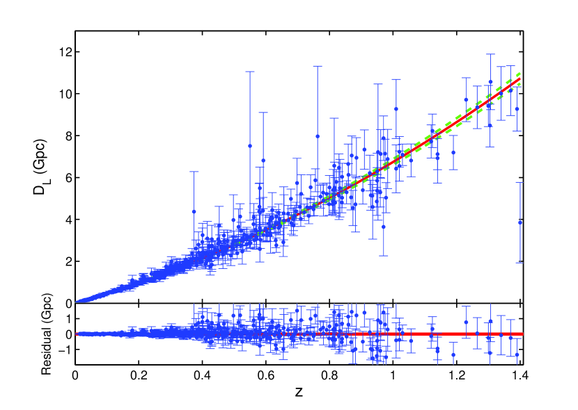
In realizing method (I), a quadratic fit is applied to all the data with errors under the principle of weighted least-squares fitting (in other words, fitting (Press et al., 1992)). The fitting curve and its CL are plotted along with the original data in Figure 1.
As suggested by others (Holanda et al., 2010; Li et al., 2011), the criterion is employed to select SNe Ia data. But in method (II), we take an inverse variance weighted average of all the selected data in the following manner. Assuming that represents th appropriate SNe Ia luminosity distance data (within ) with denoting its reported observational uncertainty, in light of conventional data reduction techniques by Bevington & Robinson (2003, Chap. 4), it is straightforward to obtain
| (2) |
where stands for the weighted mean luminosity distance at the corresponding galaxy cluster redshift, and is its uncertainty.
To get reasonable results for cluster , one has to assume certain cluster morphologies. The structure of clusters is an essential cosmological probe, as it plays important roles in discriminating different cosmological models via the mass density of the universe (Richstone et al., 1992; Suwa et al., 2003), and constraining the halo evolution models (Jing & Suto, 2002). Moreover, different assumptions of cluster shape affect the measurements of baryon fraction significantly (Cooray, 1998; Allen et al., 2004). Generally speaking, a robust way to measure cluster is through the joint analysis of X-ray emission and SZE. The hot intracluster medium interacts with CMB photons via inverse Compton scattering, causing a change in the apparent brightness of CMB and a small distortion of CMB spectrum, i.e. the SZE (Sunyaev & Zel’dovich, 1972; Birkinshaw, 1999)(also see Carlstrom et al., 2002, for a recent review). This effect is insensitive to the redshift of galaxy clusters, particularly at high redshifts () (Carlstrom et al., 2002). In calculating thermal SZE, one should consider the relativistic corrections. Itoh et al. (1998) proposed a convenient analytical expression up to fifth order terms in . If the peculiar velocity of clusters is non-negligible, namely the kinematic SZE, the relativistic corrections are presented by Nozawa et al. (1998). Mostly recently, Nozawa et al. (2006) improve these corrections to fourth order in .
Two cluster models under different morphological hypotheses are utilized. The first model involves 25 X-ray-selected clusters, with measured SZE temperature decrements (De Filippis et al., 2005). A marked triaxial ellipsoidal -model is reconstructed to describe the cluster structure, as described by
| (3) |
with defining the intrinsic orthogonal coordinates aligned with the three corresponding principal axes. represent the axial ratios (note that one of them is unity), and denotes the core radius along one of the principal axis. As a combination of Chandra, XMM-Newton and ROSAT observations, this data set consists of two sub-samples, one of which is comprised of 18 galaxy clusters with (Reese et al., 2002). The other sub-sample, analyzed by Mason et al. (2001), contains seven clusters from the X-ray flux-limited sample of Ebeling et al. (1996). The second morphological model includes 38 galaxy clusters in the redshift range from 0.14 to 0.89, provided by Bonamente et al. (2006). They modeled the electron density profile by a generalized spherical -model,
| (4) |
where and correspond to the two core radii which describe the inner and outer portions of density distribution respectively, and is a factor between zero and unity. The angular diameter distance data of every individual galaxy cluster with the two models are summarized in Table 1.
As reported by Bonamente et al. (2006), almost all angular diameter distances for the spherical -model are followed by asymmetric uncertainties. According to D’Agostini (2004), the sources of asymmetric uncertainties include non-Gaussianity of the likelihood curve, nonlinear propagation, and some systematic effects. And thus, the real value of physical quantities of interest is biased. Holanda et al. (2010) and Li et al. (2011) addressed this issue by combining the statistical and systematic uncertainties in quadrature. As stressed by Bonamente et al. (2006), the modeling uncertainties of the angular diameter distances presented in their Table 2, 4 and 5, contribute to statistical uncertainties. Therefore, it is reasonable to make the following corrections and estimations (D’Agostini, 2004, equations (15) and (16)), i.e. . We also use the reported value as the expected value () and the larger flank of each two-sided error (max()) as the standard deviation (). Hereafter we name the original spherical set the conservative spherical -model, and the set, which has been applied a moderate compensation shift to, the corrected spherical -model. Results of the angular diameter distances with conservative and corrected spherical -models are also listed in Table 1. Separately, we extract an overlap sample of clusters that are analyzed by both elliptical and spherical models. The result from the overlap sample provides a direct comparison of two morphological models of galaxy clusters.
3. Analysis Method and Results

It is straightforward to introduce the test parameter according to Eq. (1),
| (5) |
Then, the -associated one-dimensional parameterizations for are expressed as follows,
| (6a) | |||||
| (6b) | |||||
| (6c) | |||||
| (6d) | |||||
Note that can not be obtained directly from the techniques of SZE plus X-ray surface brightness observations. Uzan et al. (2004) gave a relation that describes the angular diameter distance determined from observations, i.e. , which reduces to only when , i.e. the DD relation holds with no violation. Combining this relation with Eq. (5), it is straightforward to achieve the target equation for further statistical analysis, i.e.
| (7) |
where the expression of is checked four times according to Eqs. (6a)–(6d). Maximum likelihood estimation is employed to determine the most probable values for the parameters, via and
| (8) |
where and its uncertainty is given by
| (9) |
Utilizing methods (I) and (II) described in Section 2, we are able to determine all corresponding data at each cluster’s redshift. Moreover, conservative spherical -model and corrected spherical -model are retrieved from the original data of the kpc-cut isothermal -model reported by Bonamente et al. (2006) (see Table 1). In Table 1, the number of SNe Ia selected for each galaxy cluster for method (II) analyses is also listed. For the majority of galaxy clusters, more than one SNe Ia are used. Thus the statistics is improved, especially for nearby cluster sample, e.g. Abell 1656. Because there is no SN satisfying from the cluster CL J1226.9+3332 (the nearest one is at ), this object is excluded, and also removed from method (I) analyses for the sake of direct comparison between our two methods. Our methods not only avoid double counting of any SNe Ia data, but also take into account all possible clusters data.
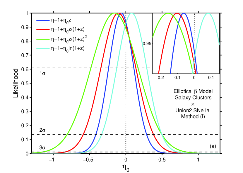
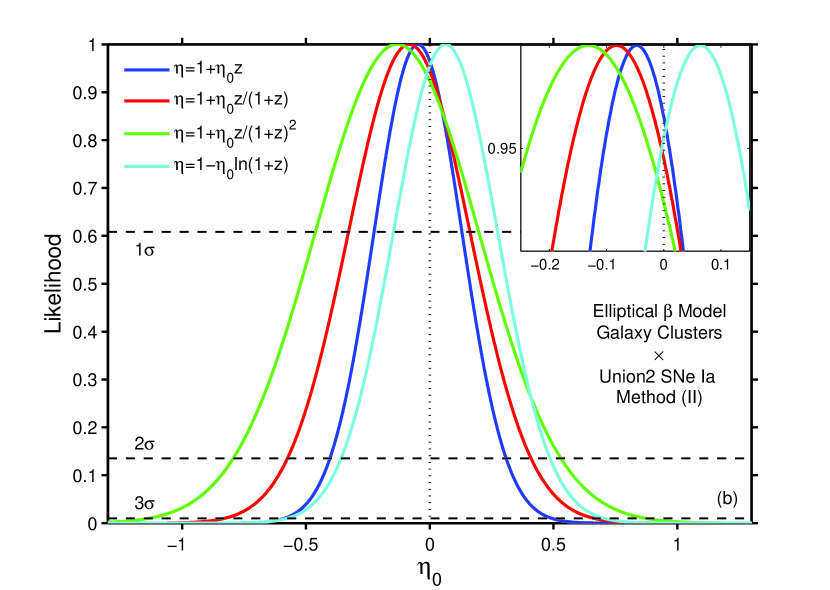
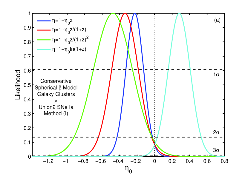
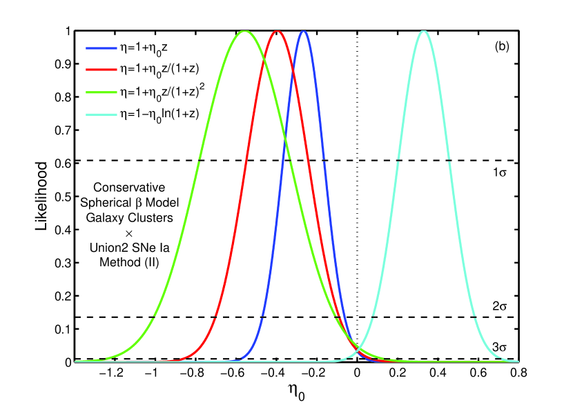
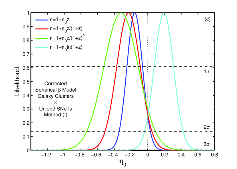
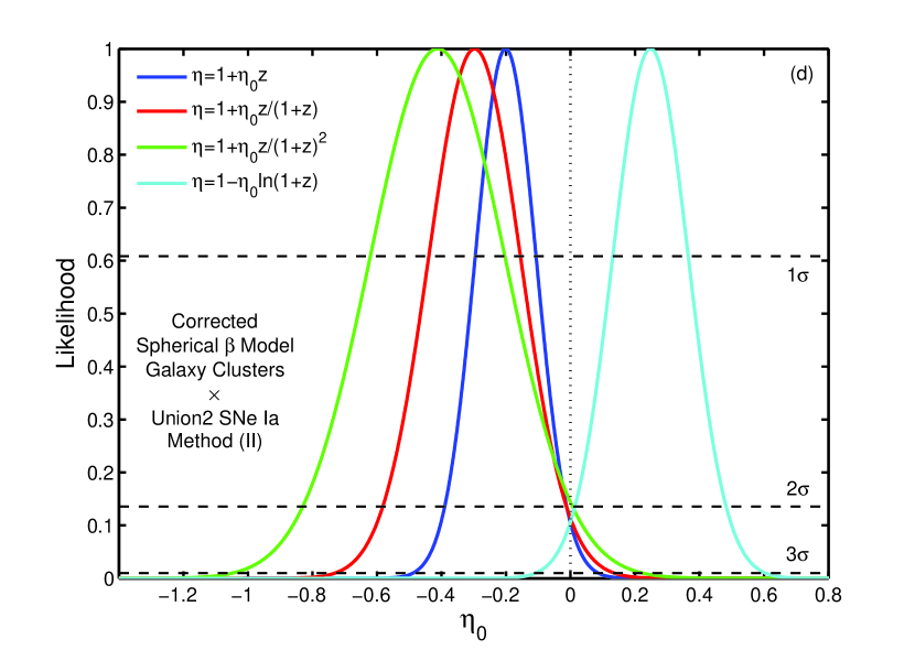
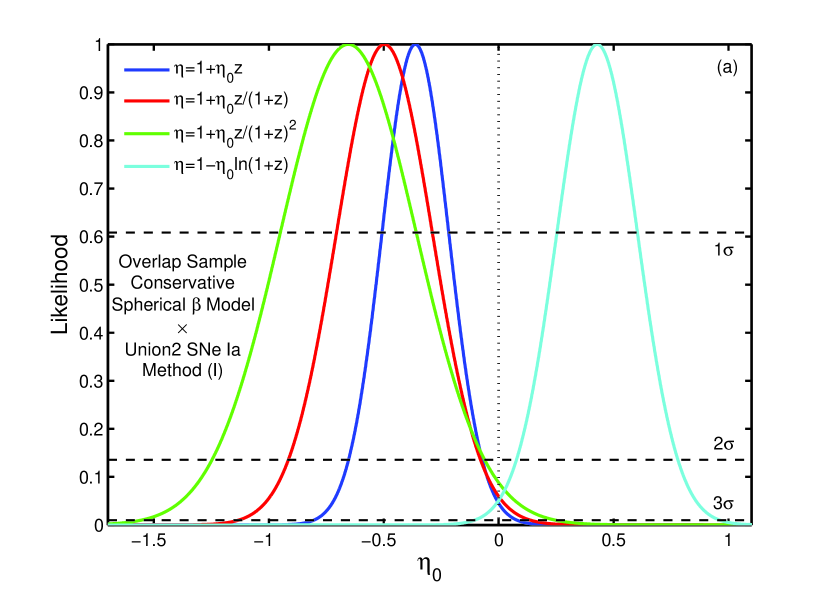
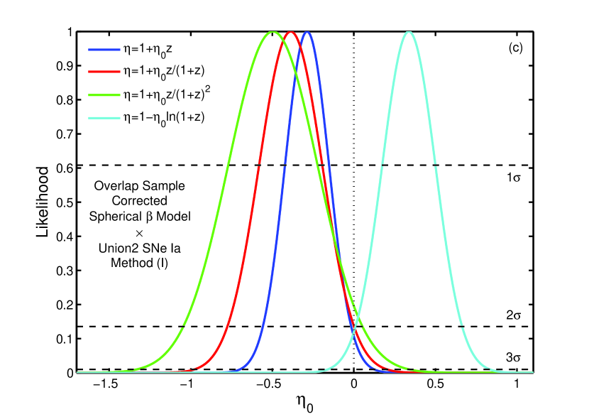
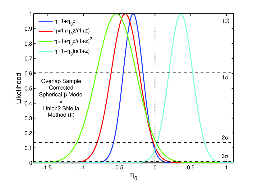
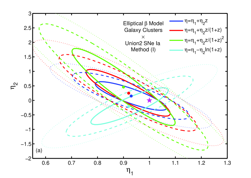
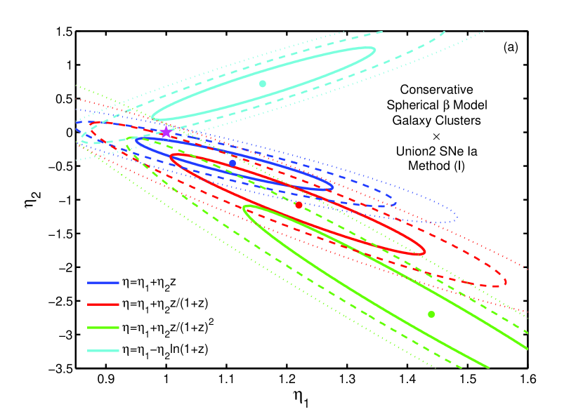
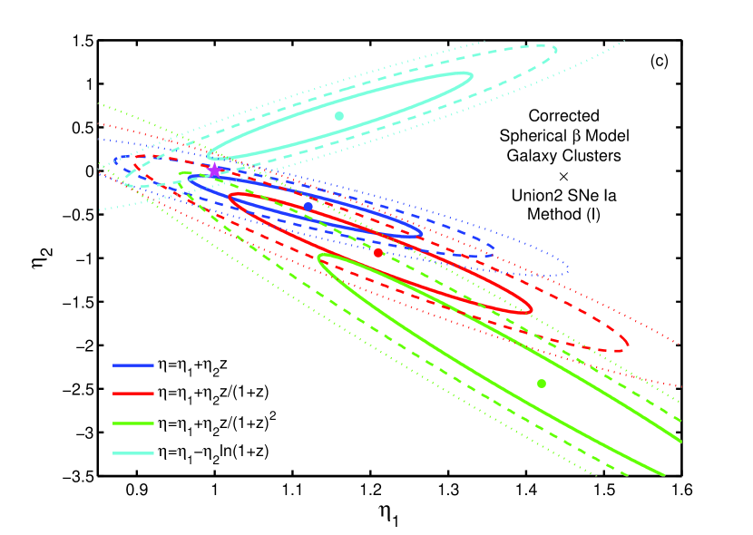
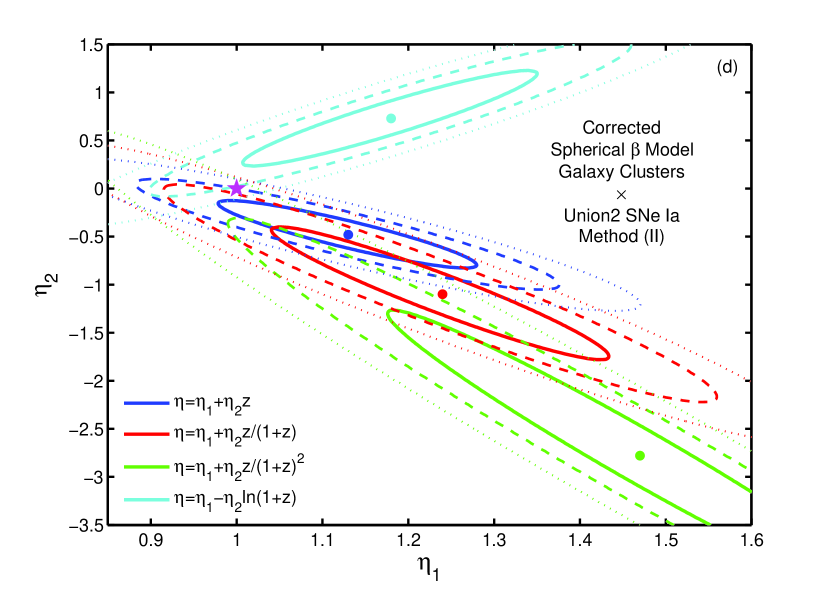
According to the results shown in Figure 2 and Table 2, the consistency is clear between the DD relation and the elliptical geometry hypothesis, since the DD relation value () is always within CL of the best-fit values of elliptical -model using both methods. However the best-fit values of conservative and corrected spherical -models depart from at nearly CL (see Figure 3), especially for conservative spherical -model (both methods) and corrected spherical -model (method (II)).
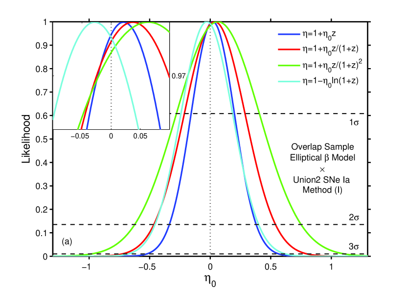
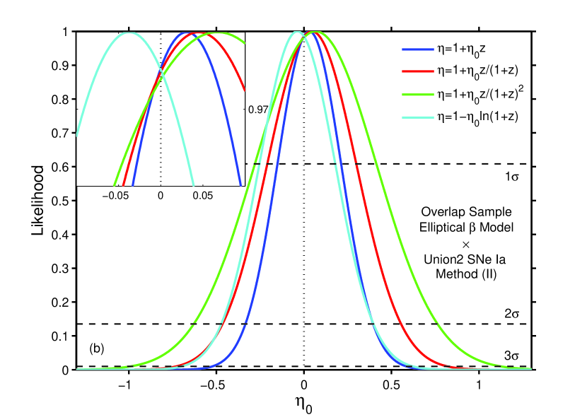
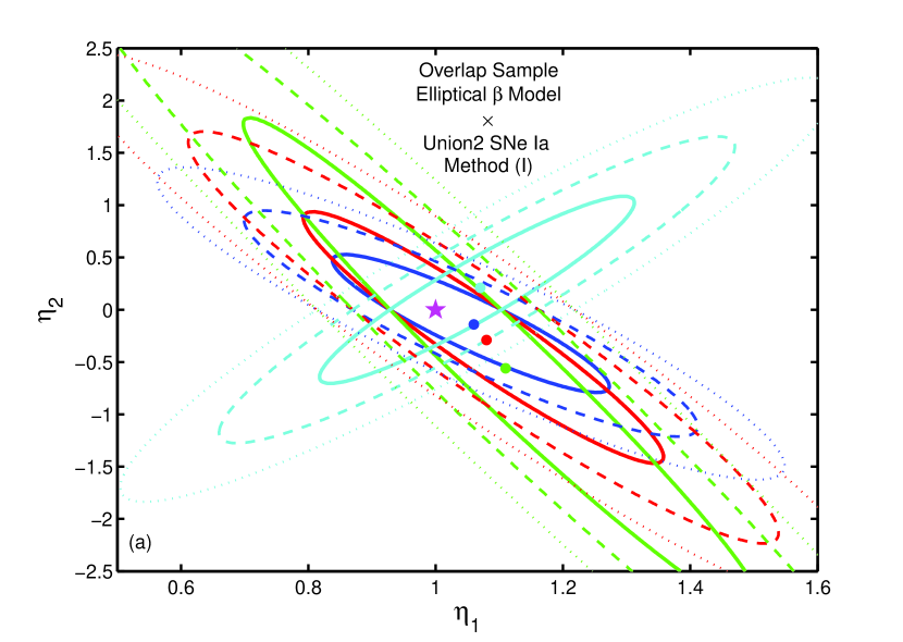
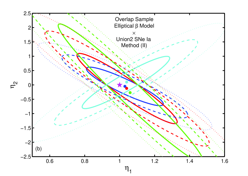
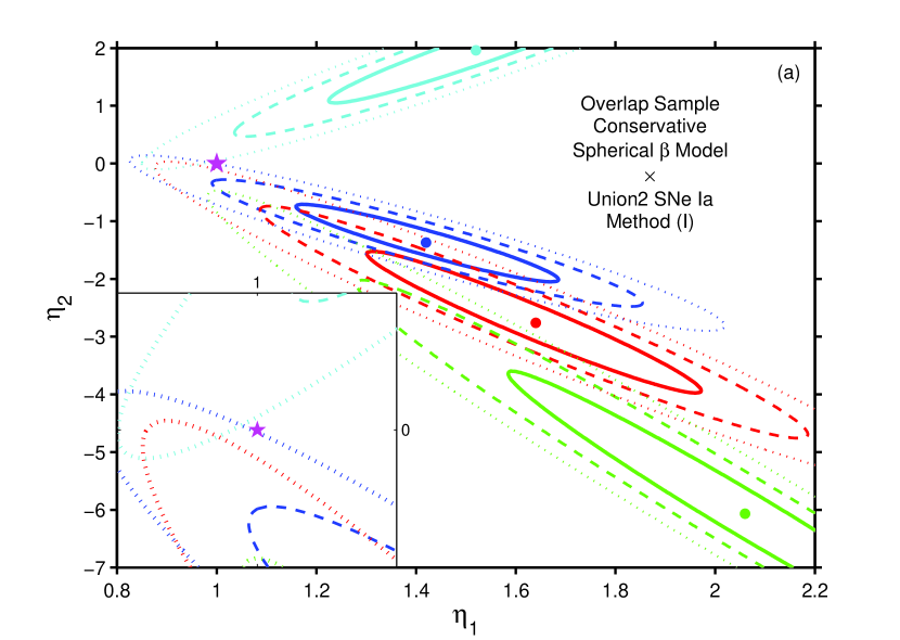
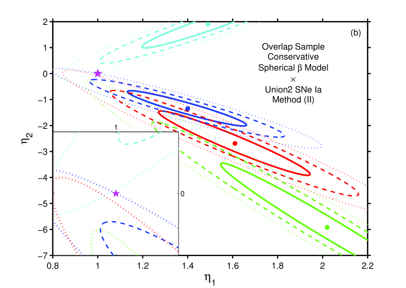
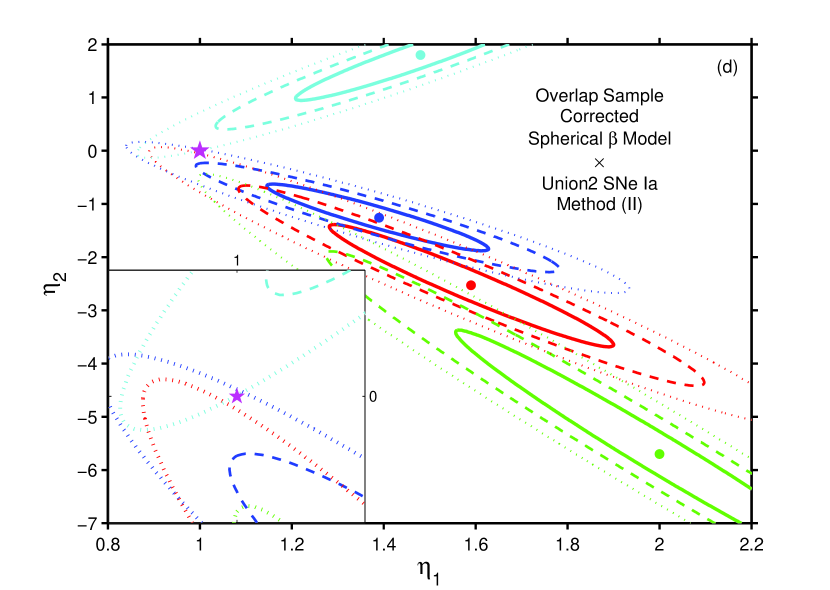
As to the overlap sample, the difference between the two morphological models are more prominent. Figure 4 demonstrates good consistency between elliptical -model and the DD relation, with the best-fit values for all parameterizations close to the DD relation value (). For the two spherical models, the results in Figure 5 show a rather marginal compatibility with the DD relation, which is slightly worse than the whole spherical sample results (see Figure 3). Statistical results of each sample using the two methods are listed in Table 2 for comparison.
The one-dimensional parameterizations of the deviation from the DD relation, i.e. in Eqs. (6a)–(6d), may be somewhat restrictive in terms of the degrees of freedom. Here the DD relation is tested with two-dimensional parameterizations of ,
| (10a) | |||||
| (10b) | |||||
| (10c) | |||||
| (10d) | |||||
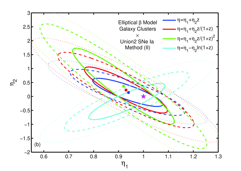
where () has the value of (1,0) if the DD relation holds. It is found that (1,0) falls in the region of all two-dimensional parameterizations for elliptical -model (Figure 6), regardless of the method used. However, for the conservative and corrected spherical -models, the DD relation can only be accommodated at CL for both methods, except the result () with method (II) for the corrected spherical -model.
The results of the two-dimensional analysis of the overlap sample (see Figures 8 and 9) are in good agreement with those of its one-dimensional analysis. In fact, the overlap sample shows a stronger preference for the elliptical geometry, as the DD relation is almost always away from the best-fit parameters for the spherical samples.
Table 3 presents the minimum values of reduced chi square () for each models with the two methods. Generally speaking, it shows the fitting quality of the corresponding models to each sample of galaxy clusters. Consistent with the results given by the best-fit values of in Table 2, the results of also favor elliptical model given the validity of DD relation, since of this model is much closer to unity than those of spherical models.
In sum, not only does spherical models have larger departures of the best-fit values of from the DD relation value () as shown in Table 2, spherical models also provide poorer fits than elliptical models do as presented in Table 3. In consequence, we argue that the galaxy cluster sample modeled by ellipsoidal morphology is a better understanding of cluster’s intrinsic nature than those modeled by spherical morphology.


4. Conclusions and Discussions
In this paper, motivated by the investigation on intrinsic structure of galaxy clusters, we have tested the validity of the DD relation using luminosity distances from Union2 SNe Ia and angular diameter distances from two cluster morphological models, namely, triaxial ellipsoidal -model and spherical -model. In order to obtain more reliable results, two sub-samples of spherical -model are analyzed according to different treatments of the two-sided errors of data, i.e. conservative and corrected spherical -models. Moreover, in order to directly compare these two types of morphological models as well as minimize systematic uncertainties of the test, we also conduct the analysis on the overlap sample, i.e. the same set of cluster individuals under both ellipsoidal and spherical -models for electron density distribution profiles.
To test the DD relation, it is assumed that . In practice, the reduction of statistical errors is realized by two methods, (I) fitting the Union2 SNe Ia data with weighted least-squares and interpolating at each cluster’s redshift, (II) binning the SNe Ia data within the redshift range to get at the cluster’s redshift. In methods (I) and (II), the parameter is parameterized in four one-dimensional forms, . Other four more general parameterizations are also considered, i.e. , which are designated to describe the two-dimensional admissible parameter space (Nair et al., 2011).
Maximum likelihood analysis is used to fit the parameters, or (, ). Our results show that for elliptical -model, regardless of whether method (I) or (II) is employed, the DD relation values ( or ) are always in region for all one- and two-dimensional forms. The results of elliptical -model support the idea that elliptical geometry is more consistent with non-violation of the DD relation. In the case of conservative spherical -model, with both methods, it is found that the DD relation value is only marginally consistent at with the best-fit values via one- and two-dimensional analyses. The result from corrected spherical -model is that the DD relation can be accommodated at CL for one-dimensional forms except using method (I), and similar results is obtained using both methods for two-dimensional parameterizations. In consequence, we can not prove that spherical -model is compatible with the validity of the DD relation.
Nevertheless, it is noticed that these results may be to some extent significantly affected by some individual data points. For instance, if cluster CL J1226.9+3332 is still included in method (I) (this object is naturally excluded in method (II) for there is no SN Ia satisfying ), the conclusion will be transformed into that the DD relation cannot be accommodated even at 3 CL for conservative spherical model. This result is tremendously different from the original results shown in Figures 3(a) and 7(a). Another example is cluster RX J1347.5-1145. If we exclude this cluster from the overlap sample, and apply our method to this new sample, the results show that for conservative spherical model the DD relation can be accommodated at 2 CL, and its give 22.470/15 and 20.204/14 for one- and two-dimensional parameterizations respectively. This result is not similar to our original results neither. Thus some thorough investigations on the influence of every cluster on the global compatibility should be paid attention to in future work.
Furthermore, it is worth making a comparison between the two methods. Our results demonstrate that the DD relation is compatible with elliptical -model at not only for one-dimensional parameterizations but also for two-dimensional forms, regardless of the methods. There is no discrepancy between the two methods for conservative spherical -model neither; the DD relation can be accommodated at with the two methods. Likewise, corrected spherical -model has approximately similar outcome, using the fitting and binning methods. The results of are similar between the two methods, as presented by Table 3. Accordingly, the two methods we used are self-consistent. With our analysis, the marked triaxial ellipsoidal model is a more reasonable hypothesis describing the structure of the galaxy cluster compared with the spherical hypothesis if the DD relation is valid in cosmological observations.
Bonamente et al. (2006) discussed the sources of some statistical and systematic uncertainties capable of affecting the angular diameter distance measurements. The main origins of systematic errors are calibrations of SZE, X-ray absolute flux and temperature, while the major statistical uncertainties come from SZE observations, X-ray spectra and images. Interestingly Bonamente et al. (2006) also pointed out that the statistical uncertainty by cluster asphericity has the largest effect, i.e. 15% on (see Table 3 of Bonamente et al., 2006), but will be averaged out when a large ensemble of clusters is considered (Sulkanen, 1999). However, our main results tell that in describing the three-dimensional morphology of galaxy clusters, the elliptical -model prevails over the spherical -models. We argue that the current cluster sample with well measured is not sufficient large to average out the uncertainty by cluster asphericity. Actually, several up-to-date observational work strongly support the triaxial ellipsoidal morphology for galaxy clusters, e.g. observations in X-ray and strong gravitational-lensing (Morandi et al., 2010), SZE imaging (Sayers et al., 2011), etc.. Recently Nagai et al. (2007) proposed another candidate profile for the distribution of intracluster medium, known as Nagai model, which is based on the well known NFW dark matter profile (Navarro et al., 1996, 1997). Although analytically non-integrable, this model can also reproduce observed intracluster medium properties through simulations. However recent observation is incapable of distinguishing between Nagai model and elliptical -model, due to limited spatial resolution (Sayers et al., 2011). Maybe with more advanced detection techniques in the future, people can learn more about the intrinsic morphology of galaxy clusters from direct observations.
References
- Allen et al. (2004) Allen, S. W., Schmidt, R. W., Ebeling, H., Fabian, A. C., & van Speybroeck, L. 2004, MNRAS, 353, 457
- Amanullah et al. (2010) Amanullah, R., et al. 2010, ApJ, 716, 712
- Avgoustidis et al. (2010) Avgoustidis, A., Burrage, C., Redondo, J., Verde, L., & Jimenez, R. 2010, JCAP, 10, 24
- Bevington & Robinson (2003) Bevington, P. R., & Robinson, D. K. 2003, Data reduction and error analysis for the physical sciences, 3rd ed., by Philip R. Bevington, and Keith D. Robinson. Boston, MA: McGraw-Hill, ISBN 0-07-247227-8
- Birkinshaw (1999) Birkinshaw, M. 1999, Phys. Rep., 310, 97
- Bonamente et al. (2006) Bonamente, M., Joy, M. K., LaRoque, S. J., Carlstrom, J. E., Reese, E. D., & Dawson, K. S. 2006, ApJ, 647, 25
- Carlstrom et al. (2002) Carlstrom, J. E., Holder, G. P., & Reese, E. D. 2002, ARA&A, 40, 643
- Cooray (1998) Cooray, A. R. 1998, A&A, 339, 623
- Cunha et al. (2007) Cunha, J. V., Marassi, L., & Lima, J. A. S. 2007, MNRAS, 379, L1
- D’Agostini (2004) D’Agostini, G. 2004, arXiv:physics/0403086
- de Bernardis et al. (2006) de Bernardis, F., Giusarma, E., & Melchiorri, A. 2006, International Journal of Modern Physics D, 15, 759
- De Filippis et al. (2005) De Filippis, E., Sereno, M., Bautz, M. W., & Longo, G. 2005, ApJ, 625, 108
- Ebeling et al. (1996) Ebeling, H., Voges, W., Bohringer, H., Edge, A. C., Huchra, J. P., & Briel, U. G. 1996, MNRAS, 281, 799
- Etherington (1933) Etherington, I. M. H. 1933, Philosophical Magazine, 15, 761
- Fox & Pen (2002) Fox, D. C., & Pen, U.-L. 2002, ApJ, 574, 38
- Freedman & Madore (2010) Freedman, W. L., & Madore, B. F. 2010, ARA&A, 48, 673
- Gavazzi (2005) Gavazzi, R. 2005, A&A, 443, 793
- Ho et al. (2006) Ho, S., Bahcall, N., & Bode, P. 2006, ApJ, 647, 8
- Holanda et al. (2010) Holanda, R. F. L., Lima, J. A. S., & Ribeiro, M. B. 2010, ApJ, 722, L233
- Holanda et al. (2011) Holanda, R. F. L., Lima, J. A. S., & Ribeiro, M. B. 2011, A&A, 528, L14
- Itoh et al. (1998) Itoh, N., Kohyama, Y., & Nozawa, S. 1998, ApJ, 502, 7
- Jing & Suto (2002) Jing, Y. P., & Suto, Y. 2002, ApJ, 574, 538
- Kasun & Evrard (2005) Kasun, S. F., & Evrard, A. E. 2005, ApJ, 629, 781
- Komatsu et al. (2011) Komatsu, E., et al. 2011, ApJS, 192, 18
- Lee & Suto (2004) Lee, J., & Suto, Y. 2004, ApJ, 601, 599
- Li et al. (2011) Li, Z., Wu, P., & Yu, H. 2011, ApJ, 729, L14
- Mason et al. (2001) Mason, B. S., Myers, S. T., & Readhead, A. C. S. 2001, ApJ, 555, L11
- Mohr et al. (1995) Mohr, J. J., Evrard, A. E., Fabricant, D. G., & Geller, M. J. 1995, ApJ, 447, 8
- Morandi et al. (2007) Morandi, A., Ettori, S., & Moscardini, L. 2007, MNRAS, 379, 518
- Morandi et al. (2010) Morandi, A., Pedersen, K., & Limousin, M. 2010, ApJ, 713, 491
- Nagai et al. (2007) Nagai, D., Kravtsov, A. V., & Vikhlinin, A. 2007, ApJ, 668, 1
- Nair et al. (2011) Nair, R., Jhingan, S., & Jain, D. 2011, JCAP, 5, 23
- Navarro et al. (1996) Navarro, J. F., Frenk, C. S., & White, S. D. M. 1996, ApJ, 462, 563
- Navarro et al. (1997) Navarro, J. F., Frenk, C. S., & White, S. D. M. 1997, ApJ, 490, 493
- Nozawa et al. (1998) Nozawa, S., Itoh, N., & Kohyama, Y. 1998, ApJ, 508, 17
- Nozawa et al. (2006) Nozawa, S., Itoh, N., Suda, Y., & Ohhata, Y. 2006, Nuovo Cimento B Serie, 121, 487
- Piffaretti et al. (2003) Piffaretti, R., Jetzer, P., & Schindler, S. 2003, A&A, 398, 41
- Press et al. (1992) Press, W. H., Teukolsky, S. A., Vetterling, W. T., & Flannery, B. P. 1992, Cambridge: University Press
- Prokhorov et al. (2011) Prokhorov, D. A., Dubois, Y., Nagataki, S., Akahori, T., & Yoshikawa, K. 2011, MNRAS, 803
- Puchwein & Bartelmann (2006) Puchwein, E., & Bartelmann, M. 2006, A&A, 455, 791
- Puchwein & Bartelmann (2007) Puchwein, E., & Bartelmann, M. 2007, A&A, 474, 745
- Reese et al. (2000) Reese, E. D., et al. 2000, ApJ, 533, 38
- Reese et al. (2002) Reese, E. D., Carlstrom, J. E., Joy, M., Mohr, J. J., Grego, L., & Holzapfel, W. L. 2002, ApJ, 581, 53
- Riess et al. (2011) Riess, A. G., et al. 2011, ApJ, 730, 119
- Richstone et al. (1992) Richstone, D., Loeb, A., & Turner, E. L. 1992, ApJ, 393, 477
- Sayers et al. (2011) Sayers, J., Golwala, S. R., Ameglio, S., & Pierpaoli, E. 2011, ApJ, 728, 39
- Schneider et al. (1999) Schneider, P., Ehlers, J., & Falco, E. E. 1999, Gravitational Lenses (New York: Springer)
- Sereno (2007) Sereno, M. 2007, MNRAS, 380, 1207
- Shang et al. (2009) Shang, C., Haiman, Z., & Verde, L. 2009, MNRAS, 400, 1085
- Stocke et al. (1991) Stocke, J. T., Morris, S. L., Gioia, I. M., Maccacaro, T., Schild, R., Wolter, A., Fleming, T. A., & Henry, J. P. 1991, ApJS, 76, 813
- Struble & Rood (1999) Struble, M. F., & Rood, H. J. 1999, ApJS, 125, 35
- Sulkanen (1999) Sulkanen, M. E. 1999, ApJ, 522, 59
- Sunyaev & Zel’dovich (1972) Sunyaev, R. A., & Zel’dovich, Y. B. 1972, Comments on Astrophysics and Space Physics, 4, 173
- Suwa et al. (2003) Suwa, T., Habe, A., Yoshikawa, K., & Okamoto, T. 2003, ApJ, 588, 7
- Thomas et al. (1998) Thomas, P. A., et al. 1998, MNRAS, 296, 1061
- Uzan et al. (2004) Uzan, J.-P., Aghanim, N., & Mellier, Y. 2004, Phys. Rev. D, 70, 083533
| Name | num | num | num | |||||
|---|---|---|---|---|---|---|---|---|
| Mpc | Mpc | Mpc | Mpc | |||||
| Overlap Sample | ||||||||
| MS 1137.5+6625 | 0.784 | 2 | 2 | 2 | ||||
| MS 0451.6-0305 | 0.550 | 5 | 5 | 5 | ||||
| CL 0016+1609 | 0.541f | 4 | 4 | 3 | ||||
| RX J1347.5-1145 | 0.451 | 7 | 7 | 7 | ||||
| Abell 370 | 0.374f | 2 | 2 | 2 | ||||
| MS 1358.4+6245 | 0.327 | 3 | 3 | 3 | ||||
| Abell 1995 | 0.322 | 3 | 3 | 3 | ||||
| Abell 611 | 0.288 | 5 | 5 | 3 | ||||
| Abell 697 | 0.282 | 6 | 6 | 6 | ||||
| Abell 1835 | 0.252 | 6 | 6 | 5 | ||||
| Abell 2261 | 0.224 | 1 | 1 | 1 | ||||
| Abell 773 | 0.217f | 12 | 12 | 12 | ||||
| Abell 2163 | 0.202 | 5 | 5 | 5 | ||||
| Abell 1689 | 0.183 | 5 | 5 | 5 | ||||
| Abell 665 | 0.182 | 5 | 5 | 5 | ||||
| Abell 2218 | 0.176f | 5 | 5 | 3 | ||||
| Abell 1413 | 0.142 | 5 | 5 | 5 | ||||
| Elliptical -model only | ||||||||
| Abell 520 | 0.202 | 5 | ||||||
| Abell 2142 | 0.091 | 4 | ||||||
| Abell 478 | 0.088 | 4 | ||||||
| Abell 1651 | 0.084 | 1 | ||||||
| Abell 401 | 0.074 | 4 | ||||||
| Abell 399 | 0.072 | 5 | ||||||
| Abell 2256 | 0.058 | 9 | ||||||
| Abell 1656 | 0.023 | 50 | ||||||
| Spherical -model only | ||||||||
| CL J1226.9+3332 | 0.890 | 0g | ||||||
| MS 1054.5-0321 | 0.826 | 3 | ||||||
| RX J1716.4+6708 | 0.813 | 6 | ||||||
| MACS J0744.8+3927 | 0.686 | 4 | ||||||
| MACS J0647.7+7015 | 0.584 | 8 | ||||||
| MS 2053.7-0449 | 0.583 | 8 | ||||||
| MACS J2129.4-0741 | 0.570 | 4 | ||||||
| MACS J1423.8+2404 | 0.545 | 1 | ||||||
| MACS J1149.5+2223 | 0.544 | 1 | ||||||
| MACS J1311.0-0310 | 0.490 | 2 | ||||||
| MACS J2214.9-1359 | 0.483 | 2 | ||||||
| MACS J2228.5+2036 | 0.412 | 6 | ||||||
| ZW 3146 | 0.291 | 3 | ||||||
| Abell 68 | 0.255 | 6 | ||||||
| RX J2129.7+0005 | 0.235 | 2 | ||||||
| Abell 267 | 0.230 | 1 | ||||||
| Abell 2111 | 0.229 | 1 | ||||||
| Abell 586 | 0.171 | 2 | ||||||
| Abell 1914 | 0.171 | 2 | ||||||
| Abell 2259 | 0.164 | 3 | ||||||
| Abell 2204 | 0.152 | 5 | ||||||
| Elliptical -model | Conservative Spherical -model | Corrected Spherical -model | ||||
|---|---|---|---|---|---|---|
| Parameterization | Method (I) | Method (II) | Method (I) | Method (II) | Method (I) | Method (II) |
| Whole Sample | ||||||
| Overlap Sample | ||||||
| Elliptical -model | Conservative Spherical -model | Corrected Spherical -model | ||||
|---|---|---|---|---|---|---|
| Parameterization | Method (I) | Method (II) | Method (I) | Method (II) | Method (I) | Method (II) |
| Whole Sample | ||||||
| 24.745/23 | 22.031/23 | 68.916/32 | 66.265/32 | 81.575/32 | 77.514/32 | |
| 24.696/23 | 21.989/23 | 68.983/32 | 66.422/32 | 81.640/32 | 77.678/32 | |
| 24.645/23 | 21.943/23 | 69.370/32 | 66.971/32 | 81.936/32 | 78.151/32 | |
| 24.719/23 | 22.009/23 | 68.903/32 | 66.290/32 | 81.573/32 | 77.553/32 | |
| 24.126/22 | 21.566/22 | 67.809/31 | 64.947/31 | 80.181/31 | 75.829/31 | |
| 24.104/22 | 21.576/22 | 66.525/31 | 63.528/31 | 78.866/31 | 74.334/31 | |
| 24.069/22 | 21.588/22 | 64.748/31 | 61.592/31 | 76.988/31 | 72.241/31 | |
| 24.118/22 | 21.573/22 | 67.150/31 | 64.219/31 | 79.508/31 | 75.066/31 | |
| Overlap Sample | ||||||
| 13.980/16 | 12.725/16 | 48.284/16 | 46.460/16 | 56.947/16 | 54.320/16 | |
| 13.972/16 | 12.722/16 | 48.837/16 | 46.971/16 | 57.464/16 | 54.800/16 | |
| 13.960/16 | 12.717/16 | 49.626/16 | 47.735/16 | 58.170/16 | 55.493/16 | |
| 13.976/16 | 12.724/16 | 48.537/16 | 46.689/16 | 57.186/16 | 54.536/16 | |
| 13.832/15 | 12.683/15 | 42.376/15 | 41.302/15 | 50.079/15 | 48.419/15 | |
| 13.811/15 | 12.673/15 | 40.559/15 | 39.517/15 | 48.033/15 | 46.418/15 | |
| 13.803/15 | 12.664/15 | 38.222/15 | 37.195/15 | 45.378/15 | 43.785/15 | |
| 13.819/15 | 12.678/15 | 41.433/15 | 40.378/15 | 49.018/15 | 47.384/15 | |