Numerical shadow and geometry of quantum states

Charles F. Dunkl1, Piotr Gawron2, John A. Holbrook3, Jarosław A. Miszczak2, Zbigniew Puchała2 and Karol Życzkowski4,5 1 Department of Mathematics, University of Virginia, Charlottesville, VA 22904—4137, USA 2 Institute of Theoretical and Applied Informatics, Polish Academy of Sciences, Bałtycka 5, 44-100 Gliwice, Poland 3 Department of Mathematics and Statistics, University of Guelph, Guelph, Ontario, N1G 2W1, Canada 4 Institute of Physics, Jagiellonian University, Reymonta 4, 30-059 Kraków, Poland 5 Center for Theoretical Physics, Polish Academy of Sciences, Aleja Lotników 32/44, 02-668 Warszawa, Poland cfd5z@virginia.edu  gawron@iitis.pl  jholbroo@uoguelph.ca  miszczak@iitis.pl  z.puchala@iitis.pl  karol@tatry.if.uj.edu.pl
Abstract

The totality of normalised density matrices of order N𝑁N forms a convex set 𝒬Nsubscript𝒬𝑁{\cal Q}_{N} in N21superscriptsuperscript𝑁21{\mathbbm{R}}^{N^{2}-1}. Working with the flat geometry induced by the Hilbert–Schmidt distance we consider images of orthogonal projections of 𝒬Nsubscript𝒬𝑁{\cal Q}_{N} onto a two–plane and show that they are similar to the numerical ranges of matrices of order N𝑁N. For a matrix A𝐴A of a order N𝑁N one defines its numerical shadow as a probability distribution supported on its numerical range W(A)𝑊𝐴W(A), induced by the unitarily invariant Fubini–Study measure on the complex projective manifold PN1superscript𝑃𝑁1{\mathbbm{C}}P^{N-1}. We define generalized, mixed–states shadows of A𝐴A and demonstrate their usefulness to analyse the structure of the set of quantum states and unitary dynamics therein.

pacs:
02.10.Yn, 02.30.Tb, 03.67.-a

April 14, 2011

1 Introduction

Investigation of the geometry of the set of quantum states remains a subject of current scientific interests in view of possible applications in the theory of quantum information processing. The set ΩNsubscriptΩ𝑁\Omega_{N} of pure quantum states belonging to a N𝑁N dimensional complex Hilbert space Nsubscript𝑁{\cal H}_{N} is known to be equivalent to the complex projective space, ΩN=PN1subscriptΩ𝑁superscript𝑃𝑁1\Omega_{N}={\mathbbm{C}}P^{N-1}, of 2N22𝑁22N-2 real dimensions. However, as this set is embedded into the N21superscript𝑁21N^{2}-1 dimensional set 𝒬Nsubscript𝒬𝑁{\cal Q}_{N} of density matrices of size N𝑁N by a non-linear constraint, ρ=ρ2𝜌superscript𝜌2\rho=\rho^{2}, the geometric structure of the set of mixed quantum states is rather involved [1, 2]. The only simple case corresponds to the one–qubit system, N=2𝑁2N=2.

The set Ω2subscriptΩ2\Omega_{2} of N=2𝑁2N=2 pure states forms the Bloch sphere, P1=S2superscript𝑃1superscript𝑆2{\mathbbm{C}}P^{1}=S^{2}, with respect to the standard Hilbert-Schmidt metric. The 333-disk inside the sphere, often called the Bloch ball, represents the set 𝒬2subscript𝒬2{\cal Q}_{2} of one–qubit mixed states. In this simple case any projection of this set onto a plane forms an ellipse, which can be degenerated to an interval. In the case of N=3𝑁3N=3 the 888 dimensional set 𝒬3subscript𝒬3{\cal Q}_{3} of one–qutrit mixed states is neither a polytope nor an ellipsoid [3, 4, 5], and the set Ω3=P2subscriptΩ3superscript𝑃2\Omega_{3}={\mathbbm{C}}P^{2} of its extremal states is connected and has four real dimensions.

Due to the high dimensionality of the problem our understanding of the geometry of the set 𝒬Nsubscript𝒬𝑁{\cal Q}_{N} of mixed states is still rather limited. This set forms a convex body which contains an in–ball of radius rN=1/N(N1)subscript𝑟𝑁1𝑁𝑁1r_{N}=\sqrt{1/N(N-1)} and can be inscribed into an out–sphere of radius RN=(N1)rN=(N1)/Nsubscript𝑅𝑁𝑁1subscript𝑟𝑁𝑁1𝑁R_{N}=(N-1)r_{N}=\sqrt{(N-1)/N} [2]. Some information on the subject can be gained by studying the 222–dimensional cross-sections of 𝒬Nsubscript𝒬𝑁{\cal Q}_{N} as demonstrated in [6, 7, 8] for N=3𝑁3N=3 and N=4𝑁4N=4. Another option is to investigate projections of this set into a plane – such an approach was advocated for N=3𝑁3N=3 in [9]. As the set 𝒬Nsubscript𝒬𝑁{\cal Q}_{N} of quantum states is convex, also its cross-sections and projections inherit convexity.

In this work we study the general structure of a two–dimensional projection of the set 𝒬Nsubscript𝒬𝑁{\cal Q}_{N} of mixed states. A bridge between the geometry of the set of quantum states and the notion of numerical range used in operator theory is established. For any operator A𝐴A, acting on the complex Hilbert space Nsubscript𝑁{\cal H}_{N}, one defines its numerical range [10, 11] (also called field of values) as a subset of the complex plane which contains expectation values of A𝐴A among arbitrary normalized pure states,

W(A)={z:z=ψ|A|ψ,|ψN,ψ|ψ=1}.𝑊𝐴conditional-set𝑧formulae-sequence𝑧quantum-operator-product𝜓𝐴𝜓formulae-sequenceket𝜓subscript𝑁inner-product𝜓𝜓1W(A)=\{z:z=\langle\psi|A|\psi\rangle,\ |\psi\rangle\in{\cal H}_{N},\ \langle\psi|\psi\rangle=1\}. (1)

We analyse the set of orthogonal projections of the set 𝒬Nsubscript𝒬𝑁{\cal Q}_{N} onto a 222–plane and prove that it is equivalent to the set of all possible numerical ranges of complex matrices of order N𝑁N. Numerical ranges of normal matrices of size N𝑁N correspond to orthogonal projections of the set 𝒞Nsubscript𝒞𝑁{\cal C}_{N} of classical states – the (N1)𝑁1(N-1)-dimensional simplex ΔN1N1subscriptΔ𝑁1superscript𝑁1\Delta_{N-1}\subset{\mathbb{R}}^{N-1}.

Further information on the structure of the set of quantum states of a size N𝑁N can be obtained by studying the numerical shadow [12, 13, 14] of various matrices of order N𝑁N. For any operator A𝐴A acting on Nsubscript𝑁{\cal H}_{N} one defines a probability distribution PA(z)subscript𝑃𝐴𝑧P_{A}(z) on the complex plane, supported in the numerical range W(A)𝑊𝐴W(A),

PA(z):=ΩNdμ(ψ)δ(zψ|A|ψ).assignsubscript𝑃𝐴𝑧subscriptsubscriptΩ𝑁differential-d𝜇𝜓𝛿𝑧quantum-operator-product𝜓𝐴𝜓P_{A}(z):=\int_{\Omega_{N}}{\rm d}\mu(\psi)\delta\Bigl{(}z-\langle\psi|A|\psi\rangle\Bigr{)}. (2)

Here μ(ψ)𝜇𝜓\mu(\psi) denotes the unique unitarily invariant (Fubini-Study) measure on the set ΩNsubscriptΩ𝑁\Omega_{N} of N𝑁N-dimensional pure quantum states. In other words the shadow P𝑃P of matrix A𝐴A at a given point z𝑧z characterizes the likelihood that the expectation value of A𝐴A among a random pure state is equal to z𝑧z.

The distribution PA(z)subscript𝑃𝐴𝑧P_{A}(z) is naturally associated a given matrix A𝐴A, and some of its properties were described in [13]. In this work we advocate a complementary approach and show that investigating the shadows of several different complex matrices A𝐴A of a fixed size N𝑁N contributes to our understanding of the structure of the entire set 𝒬Nsubscript𝒬𝑁{\cal Q}_{N} of quantum states. In a sense, the choice of a matrix A𝐴A corresponds to the selection of the plane, onto which the set of quantum states is projected.

This paper is organized as follows. In section 2 we fix the notation and introduce necessary concepts. A link between 222–dimensional projections of the set of quantum states of a given size N𝑁N and the set of possible numerical ranges of matrices of order N𝑁N is presented in section 3. In section 4 we analyze different classes of numerical shadows of matrices of small order N=2,3,4𝑁234N=2,3,4. Unitary dynamics of a pure quantum state in the background of numerical shadow is presented in section 5. Section 6 is devoted to the mixed–states numerical shadow, which corresponds to a projection of the full set 𝒬Nsubscript𝒬𝑁{\cal Q}_{N} of density matrices onto a plane. The case of a large dimension, N1much-greater-than𝑁1N\gg 1, is treated in section 7 jointly with the shadow of random matrices. Finally, in section 8 we provide some concluding remarks and summarize the contribution of this paper.

2 Classical and quantum states

Let p={x1,x2,,xN}𝑝subscript𝑥1subscript𝑥2subscript𝑥𝑁p=\{x_{1},x_{2},\dots,x_{N}\} be a normalized probability vector, so xi0subscript𝑥𝑖0x_{i}\geq 0 and i=1Nxi=1superscriptsubscript𝑖1𝑁subscript𝑥𝑖1\sum_{i=1}^{N}x_{i}=1. Such a vector represents a classical state, and the set 𝒞Nsubscript𝒞𝑁{\cal C}_{N} of all classical states forms an (N1)𝑁1(N-1) dimensional regular simplex ΔN1N1subscriptΔ𝑁1superscript𝑁1\Delta_{N-1}\subset{\mathbbm{R}}^{N-1}. There exist exactly N𝑁N classical pure states, which correspond to the corners of the simplex. All other classical states can be expressed by a convex combination of pure states and are called mixed. Typical mixed states are characterized by the full rank and they form the entire interior of the probability simplex.

In quantum theory one describes a physical system with N𝑁N distinguishable states by elements of a complex Hilbert space Nsubscript𝑁{\cal H}_{N} of size N𝑁N. Its elements represent pure quantum states, |ψNket𝜓subscript𝑁|\psi\rangle\in{\cal H}_{N}. Quantum states are assumed to be normalized, ψ2=ψ|ψ=1superscriptnorm𝜓2inner-product𝜓𝜓1||\psi||^{2}=\langle\psi|\psi\rangle=1, so they belong to the sphere of dimension 2N12𝑁12N-1. Since one identifies two states, which differ by a global phase only, |ψ|ϕ=eα|ψsimilar-toket𝜓ketitalic-ϕsuperscript𝑒𝛼ket𝜓|\psi\rangle\sim|\phi\rangle=e^{-\alpha}|\psi\rangle, the set of all pure quantum states ΩNsubscriptΩ𝑁\Omega_{N}, which act on Nsubscript𝑁{\cal H}_{N}, is equivalent to the complex projective space, ΩN=PN1subscriptΩ𝑁superscript𝑃𝑁1\Omega_{N}={\mathbbm{C}}P^{N-1} [2].

In analogy to the classical case, one also defines mixed quantum states (density matrices) by a convex combination of projectors onto pure states, ρ=ipi|ψiψi|𝜌subscript𝑖subscript𝑝𝑖ketsubscript𝜓𝑖brasubscript𝜓𝑖\rho=\sum_{i}p_{i}|\psi_{i}\rangle\langle\psi_{i}|, where pi>0subscript𝑝𝑖0p_{i}>0 and ipi=1subscript𝑖subscript𝑝𝑖1\sum_{i}p_{i}=1. Let us denote the set of all density matrices of order N𝑁N by 𝒬Nsubscript𝒬𝑁{\cal Q}_{N}. It contains all density operators which are positive and normalized,

𝒬N={ρ:NN,ρ=ρ,ρ0,Trρ=1}.subscript𝒬𝑁conditional-set𝜌formulae-sequencesubscript𝑁subscript𝑁formulae-sequencesuperscript𝜌𝜌formulae-sequence𝜌0Tr𝜌1{\cal Q}_{N}=\{\rho:{\cal H}_{N}\to{\cal H}_{N},\quad\rho^{*}=\rho,\quad\rho\geq 0,\quad{\rm Tr}\rho=1\}\;. (3)

Since density operators are Hermitian and normalized, this set is N21superscript𝑁21N^{2}-1 dimensional. It includes the set of classical states, 𝒬N𝒞N=ΔN1superset-ofsubscript𝒬𝑁subscript𝒞𝑁subscriptΔ𝑁1{\cal Q}_{N}\supset{\cal C}_{N}=\Delta_{N-1}, as well as the set of pure quantum states, 𝒬NΩN=PN1superset-ofsubscript𝒬𝑁subscriptΩ𝑁superscript𝑃𝑁1{\cal Q}_{N}\supset\Omega_{N}={\mathbbm{C}}P^{N-1}. We are going to work with the geometry implied by the Hilbert–Schmidt norm of a matrix, |A|HS:=Tr(AA)assignsubscript𝐴HSTrsuperscript𝐴𝐴|A|_{\rm HS}:=\sqrt{\mathrm{Tr}(A^{\ast}A)}, and the Hilbert-Schmidt distance in the space of matrices,

dHS(A,B):=|AB|HS=Tr(AB)(AB).assignsubscript𝑑HS𝐴𝐵subscript𝐴𝐵HSTr𝐴𝐵superscript𝐴𝐵d_{\rm HS}(A,B):=|A-B|_{\rm HS}=\sqrt{\mathrm{Tr}(A-B)(A-B)^{\ast}}. (4)

It will be also convenient to define a real inner-product by setting the polar identity

A,B=14|A+B|HS214|AB|HS2=12[Tr(AB+BA)].𝐴𝐵14superscriptsubscript𝐴𝐵HS214superscriptsubscript𝐴𝐵HS212delimited-[]Trsuperscript𝐴𝐵superscript𝐵𝐴\left\langle A,B\right\rangle=\frac{1}{4}|A+B|_{\rm HS}^{2}-\frac{1}{4}|A-B|_{\rm HS}^{2}=\frac{1}{2}[\mathrm{Tr}(A^{\ast}B+B^{\ast}A)]. (5)

If A=Asuperscript𝐴𝐴A^{\ast}=A and B=Bsuperscript𝐵𝐵B^{\ast}=B then A,B=trAB𝐴𝐵tr𝐴𝐵\left\langle A,B\right\rangle=\mathrm{tr}AB.

In the set ΩNsubscriptΩ𝑁\Omega_{N} of quantum pure states one defines the Fubini-Study measure μFSsubscript𝜇FS\mu_{\rm FS}, which is induced by the Haar measure on U(N)𝑈𝑁U(N) and is invariant with respect to unitary transformations. In the case of one–qubit states this measure corresponds to the uniform distribution of points on the Bloch sphere S2superscript𝑆2S^{2}.

In practice, to generate pure states at random according to the measure μFSsubscript𝜇FS\mu_{\rm FS} it is sufficient to generate uniformly points at the sphere S2N1superscript𝑆2𝑁1S^{2N-1}. One may also select an arbitrary column, (or row) of a random unitary matrix U𝑈U distributed according to the Haar measure. It directly gives the set of N𝑁N coefficients of the random state in a given basis, |ψ=i=1Nci|iket𝜓superscriptsubscript𝑖1𝑁subscript𝑐𝑖ket𝑖|\psi\rangle=\sum_{i=1}^{N}c_{i}|i\rangle. For instance, choosing the first column of U𝑈U we set ci=Ui,1subscript𝑐𝑖subscript𝑈𝑖1c_{i}=U_{i,1} for i=1,,N𝑖1𝑁i=1,\dots,N. Alternatively, one may generate N𝑁N independent complex random numbers zisubscript𝑧𝑖z_{i} and renormalise them, ci=zi/i|zi|2subscript𝑐𝑖subscript𝑧𝑖subscript𝑖superscriptsubscript𝑧𝑖2c_{i}=z_{i}/\sqrt{\sum_{i}|z_{i}|^{2}}, to obtain the desired distribution [15, 3].

In this work we are going to use the following

Proposition 1

Let |ψΩNket𝜓subscriptΩ𝑁|\psi\rangle\in\Omega_{N} be a random pure state of size N𝑁N distributed according to the Fubini-Study measure. If one represents it in an arbitrary fixed basis, |ψ=i=1Nci|iket𝜓superscriptsubscript𝑖1𝑁subscript𝑐𝑖ket𝑖|\psi\rangle=\sum_{i=1}^{N}c_{i}|i\rangle then the squared absolute values of the coefficients, pi=|ci|2subscript𝑝𝑖superscriptsubscript𝑐𝑖2p_{i}=|c_{i}|^{2}, form a probability vector distributed uniformly in the probability simplex ΔN1subscriptΔ𝑁1\Delta_{N-1}.

This is equivalent to the known statement (see e.g. [2]), that the only constraint on the components of a single column of a random unitary matrix U𝑈U distributed according to the Haar measure is the normalization condition, P(U11,UN1)δ(1i=1N|Ui1|2)similar-to𝑃subscript𝑈11subscript𝑈𝑁1𝛿1superscriptsubscript𝑖1𝑁superscriptsubscript𝑈𝑖12P(U_{11},\dots U_{N1})\sim\delta\Bigl{(}1-\sum_{i=1}^{N}|U_{i1}|^{2}\Bigr{)}. This fact directly implies

Corollary 2

For any quantum state ρ𝜌\rho define a classical state p=diag(ρ)𝑝diag𝜌p={\rm diag}(\rho), so pi=ρiisubscript𝑝𝑖subscript𝜌𝑖𝑖p_{i}=\rho_{ii}. Then the Fubini-Study measure on the set ΩNsubscriptΩ𝑁\Omega_{N} of quantum pure states induces by this mapping the uniform measure in the classical probability simplex ΔN1subscriptΔ𝑁1\Delta_{N-1}.

In the case of N=2𝑁2N=2 the Fubini-Study measure covers uniformly the Bloch sphere S2superscript𝑆2S^{2}. Working with the standard polar coordinates, (r,θ,φ)𝑟𝜃𝜑(r,\theta,\varphi), we write the element of the volume of the unit sphere as dS=dφsinθdθ=dφd(cosθ)𝑑𝑆𝑑𝜑𝜃𝑑𝜃𝑑𝜑𝑑𝜃dS=d\varphi\sin\theta d\theta=d\varphi d(\cos\theta). The polar angle θ𝜃\theta is defined with respect to the axis z𝑧z, so the projection of a point of the sphere at this axis reads z=cosθ𝑧𝜃z=\cos\theta. Hence the Fubini-Study measure implies the uniform distribution d(cosθ)=dz𝑑𝜃𝑑𝑧d(\cos\theta)=dz along the one-dimensional set Δ1subscriptΔ1\Delta_{1} of N=2𝑁2N=2 classical states.

3 Numerical range as a projection of the set of quantum states

The set ΩN=PN1subscriptΩ𝑁superscript𝑃𝑁1\Omega_{N}={\mathbbm{C}}P^{N-1} of pure states of size N𝑁N forms the set of extremal points in 𝒬Nsubscript𝒬𝑁{\cal Q}_{N}. Any mixed state ρ𝒬N𝜌subscript𝒬𝑁\rho\in{\cal Q}_{N} can be thus decomposed into a convex mixture of projectors |ψψ|ket𝜓bra𝜓|\psi\rangle\langle\psi|. The expectation value of an operator A𝐴A among a pure state reads ψ|A|ψ=TrρAquantum-operator-product𝜓𝐴𝜓Tr𝜌𝐴\langle\psi|A|\psi\rangle={\rm Tr}\rho A. Taking into account the convexity of W(A)𝑊𝐴W(A), the standard definition (1) of the numerical range of A𝐴A can be therefore rewritten as [16]

W(A)={z:z=TrρA,ρ𝒬N}.𝑊𝐴conditional-set𝑧formulae-sequence𝑧Tr𝜌𝐴𝜌subscript𝒬𝑁W(A)=\{z:z={\rm Tr}\rho A,\ \rho\in{\cal Q}_{N}\}. (6)

This expression suggests a possible link between numerical range and the structure of the set the 𝒬Nsubscript𝒬𝑁{\cal Q}_{N}. Usually one studies numerical range W(A)𝑊𝐴W(A) for a given A𝐴A [11]. Here we propose to fix the dimension N𝑁N and consider the set of all possible numerical ranges of matrices A𝐴A of this size to analyze the geometry of quantum states. More precisely, we establish the following facts.

Proposition 3

Let 𝒞Nsubscript𝒞𝑁{\cal C}_{N} denote the set of classical states of size N𝑁N, which forms the regular simplex ΔN1subscriptΔ𝑁1\Delta_{N-1} in N1superscript𝑁1{\mathbbm{R}}^{N-1}. Then the set of similar images of orthogonal projections of 𝒞Nsubscript𝒞𝑁{\cal C}_{N} on a 222–plane is equivalent to the set of all possible numerical ranges W(A)𝑊𝐴W(A) of all normal matrices A𝐴A (such that AA=AA𝐴superscript𝐴superscript𝐴𝐴AA^{*}=A^{*}A) of order N𝑁N.

Proposition 4

Let 𝒬Nsubscript𝒬𝑁{\cal Q}_{N} denote the set of quantum states size N𝑁N embedded in N21superscriptsuperscript𝑁21{\mathbbm{R}}^{N^{2}-1} with respect to Euclidean geometry induced by Hilbert-Schmidt distance. Then the set of similar images of orthogonal projections 𝒬Nsubscript𝒬𝑁{\cal Q}_{N} on a 222-plane is equivalent to the set of all possible numerical ranges W(A)𝑊𝐴W(A) of (arbitrary) matrices A𝐴A of order N𝑁N.

To prove the above propositions we will need an abstract lemma concerning the real inner-product Euclidean spaces.

Lemma 5

Suppose u1,u2,v0Vsubscript𝑢1subscript𝑢2subscript𝑣0𝑉u_{1},u_{2},v_{0}\in V, where V𝑉V is a Euclidean vector space (with inner product ,\left\langle\cdot,\cdot\right\rangle and norm |x|=x,x1/2𝑥superscript𝑥𝑥12\left|x\right|=\left\langle x,x\right\rangle^{1/2}), v00subscript𝑣00v_{0}\neq 0 and dim(span{u1,u2,v0})2dimensionspansubscript𝑢1subscript𝑢2subscript𝑣02\dim\left(\mathrm{span}\left\{u_{1},u_{2},v_{0}\right\}\right)\geq 2. Then there exist real numbers α>0,γ1,γ2𝛼0subscript𝛾1subscript𝛾2\alpha>0,\gamma_{1},\gamma_{2} such that the vectors

v1:=1α(u1+γ1v0),v2:=1α(u2+γ2v0)formulae-sequenceassignsubscript𝑣11𝛼subscript𝑢1subscript𝛾1subscript𝑣0assignsubscript𝑣21𝛼subscript𝑢2subscript𝛾2subscript𝑣0v_{1}:=\frac{1}{\alpha}\left(u_{1}+\gamma_{1}v_{0}\right),\ \ \ v_{2}:=\frac{1}{\alpha}\left(u_{2}+\gamma_{2}v_{0}\right) (7)

are normalized and orthogonal,

|v1|2=1=|v2|2,v1,v2=0.formulae-sequencesuperscriptsubscript𝑣121superscriptsubscript𝑣22subscript𝑣1subscript𝑣20\left|v_{1}\right|^{2}=1=\left|v_{2}\right|^{2},\ \ \ \left\langle v_{1},v_{2}\right\rangle=0\;. (8)

Proof. Let ui=uiui,v0|v0|2v0,i=1,2formulae-sequencesuperscriptsubscript𝑢𝑖subscript𝑢𝑖subscript𝑢𝑖subscript𝑣0superscriptsubscript𝑣02subscript𝑣0𝑖12u_{i}^{\prime}=u_{i}-\frac{\left\langle u_{i},v_{0}\right\rangle}{|v_{0}|^{2}}v_{0},\ \ i=1,2. By hypothesis |u1|2+|u2|2>0superscriptsuperscriptsubscript𝑢12superscriptsuperscriptsubscript𝑢220|u_{1}^{\prime}|^{2}+|u_{2}^{\prime}|^{2}>0. For i=1,2𝑖12i=1,2 set ci:=|v0|γi+ui,v0|v0|assignsubscript𝑐𝑖subscript𝑣0subscript𝛾𝑖subscript𝑢𝑖subscript𝑣0subscript𝑣0c_{i}:=|v_{0}|\gamma_{i}+\frac{\left\langle u_{i},v_{0}\right\rangle}{|v_{0}|} so that vi=1α(ui+ci|v0|v0)subscript𝑣𝑖1𝛼superscriptsubscript𝑢𝑖subscript𝑐𝑖subscript𝑣0subscript𝑣0v_{i}=\frac{1}{\alpha}\left(u_{i}^{\prime}+\frac{c_{i}}{|v_{0}|}v_{0}\right). The desired equations become

|u1|2+c12=α2,|u2|2+c22=α2,u1,u2+c1c2=0.formulae-sequencesuperscriptsuperscriptsubscript𝑢12superscriptsubscript𝑐12superscript𝛼2formulae-sequencesuperscriptsuperscriptsubscript𝑢22superscriptsubscript𝑐22superscript𝛼2superscriptsubscript𝑢1superscriptsubscript𝑢2subscript𝑐1subscript𝑐20|u_{1}^{\prime}|^{2}+c_{1}^{2}=\alpha^{2},\ \ |u_{2}^{\prime}|^{2}+c_{2}^{2}=\alpha^{2},\ \ \left\langle u_{1}^{\prime},u_{2}^{\prime}\right\rangle+c_{1}c_{2}=0. (9)

Eliminating coefficient α𝛼\alpha we arrive at a quadratic equation for c12superscriptsubscript𝑐12c_{1}^{2} or c22superscriptsubscript𝑐22c_{2}^{2}. Set

d=(|u1|2|u2|2)2+4u1,u22,𝑑superscriptsuperscriptsuperscriptsubscript𝑢12superscriptsuperscriptsubscript𝑢2224superscriptsuperscriptsubscript𝑢1superscriptsubscript𝑢22d=\left(|u_{1}^{\prime}|^{2}-|u_{2}^{\prime}|^{2}\right)^{2}+4\langle u_{1}^{\prime},u_{2}^{\prime}\rangle^{2},

then

c12superscriptsubscript𝑐12\displaystyle c_{1}^{2} =12(|u2|2|u1|2)+12d,absent12superscriptsuperscriptsubscript𝑢22superscriptsuperscriptsubscript𝑢1212𝑑\displaystyle=\frac{1}{2}\left(|u_{2}^{\prime}|^{2}-|u_{1}^{\prime}|^{2}\right)+\frac{1}{2}\sqrt{d}, (10)
c22superscriptsubscript𝑐22\displaystyle c_{2}^{2} =12(|u1|2|u2|2)+12d,absent12superscriptsuperscriptsubscript𝑢12superscriptsuperscriptsubscript𝑢2212𝑑\displaystyle=\frac{1}{2}\left(|u_{1}^{\prime}|^{2}-|u_{2}^{\prime}|^{2}\right)+\frac{1}{2}\sqrt{d}, (11)
sign(c1c2)signsubscript𝑐1subscript𝑐2\displaystyle\mathrm{sign}\left(c_{1}c_{2}\right) =signu1,u2,absentsignsuperscriptsubscript𝑢1superscriptsubscript𝑢2\displaystyle=-\mathrm{sign}\left\langle u_{1}^{\prime},u_{2}^{\prime}\right\rangle, (12)
α𝛼\displaystyle\alpha =(12(|u1|2+|u2|2)+12d)1/2.absentsuperscript12superscriptsuperscriptsubscript𝑢12superscriptsuperscriptsubscript𝑢2212𝑑12\displaystyle=\left(\frac{1}{2}\left(|u_{1}^{\prime}|^{2}+|u_{2}^{\prime}|^{2}\right)+\frac{1}{2}\sqrt{d}\right)^{1/2}. (13)

Recall |u1|2+|u2|2>0superscriptsuperscriptsubscript𝑢12superscriptsuperscriptsubscript𝑢220|u_{1}^{\prime}|^{2}+|u_{2}^{\prime}|^{2}>0 by hypothesis thus α>0𝛼0\alpha>0. There are generally two solutions differing only in the signs of c1subscript𝑐1c_{1} and c2subscript𝑐2c_{2}. If u1,u2=0superscriptsubscript𝑢1superscriptsubscript𝑢20\langle u_{1}^{\prime},u_{2}^{\prime}\rangle=0 then d=||u1|2|u2|2|𝑑superscriptsuperscriptsubscript𝑢12superscriptsuperscriptsubscript𝑢22\sqrt{d}=\left||u_{1}^{\prime}|^{2}-|u_{2}^{\prime}|^{2}\right|, and one of the three following cases apply:
1. |u1|>|u2|0,c1=0,c2=±|u1|2|u2|2,α=|u1|formulae-sequencesuperscriptsubscript𝑢1superscriptsubscript𝑢20formulae-sequencesubscript𝑐10formulae-sequencesubscript𝑐2plus-or-minussuperscriptsuperscriptsubscript𝑢12superscriptsuperscriptsubscript𝑢22𝛼superscriptsubscript𝑢1|u_{1}^{\prime}|>|u_{2}^{\prime}|\geq 0,\ c_{1}=0,\ c_{2}=\pm\sqrt{|u_{1}^{\prime}|^{2}-|u_{2}^{\prime}|^{2}},\ \alpha=|u_{1}^{\prime}|;
2. |u2|>|u1|0,c1=±|u2|2|u1|2,c2=0,α=|u2|formulae-sequencesuperscriptsubscript𝑢2superscriptsubscript𝑢10formulae-sequencesubscript𝑐1plus-or-minussuperscriptsuperscriptsubscript𝑢22superscriptsuperscriptsubscript𝑢12formulae-sequencesubscript𝑐20𝛼superscriptsubscript𝑢2|u_{2}^{\prime}|>|u_{1}^{\prime}|\geq 0,\ c_{1}=\pm\sqrt{|u_{2}^{\prime}|^{2}-|u_{1}^{\prime}|^{2}},\ c_{2}=0,\ \alpha=|u_{2}^{\prime}|;
3. |u1|=|u2|>0,c1=0,c2=0,α=|u1|formulae-sequencesuperscriptsubscript𝑢1superscriptsubscript𝑢20formulae-sequencesubscript𝑐10formulae-sequencesubscript𝑐20𝛼superscriptsubscript𝑢1|u_{1}^{\prime}|=|u_{2}^{\prime}|>0,\ c_{1}=0,\ c_{2}=0,\ \alpha=|u_{1}^{\prime}|.   \square

Note that the formulae (10, 11) for c1subscript𝑐1c_{1} and c2subscript𝑐2c_{2} allow us to obtain the constants γ1subscript𝛾1\gamma_{1} and γ2subscript𝛾2\gamma_{2}, which enter eq. (7). The scaling factor α=1𝛼1\alpha=1 if and only if u1,u22=(1|u1|2)(1|u2|2)superscriptsuperscriptsubscript𝑢1superscriptsubscript𝑢221superscriptsuperscriptsubscript𝑢121superscriptsuperscriptsubscript𝑢22\langle u_{1}^{\prime},u_{2}^{\prime}\rangle^{2}=(1-|u_{1}^{\prime}|^{2})(1-|u_{2}^{\prime}|^{2}), |u1|21superscriptsuperscriptsubscript𝑢121|u_{1}^{\prime}|^{2}\leq 1 and |u2|21superscriptsuperscriptsubscript𝑢221|u_{2}^{{}^{\prime}}|^{2}\leq 1.

This lemma implies the following

Corollary 6

Suppose E{xV:x,v0=1}𝐸conditional-set𝑥𝑉𝑥subscript𝑣01E\subset\left\{x\in V:\left\langle x,v_{0}\right\rangle=1\right\} and u1,u2Vsubscript𝑢1subscript𝑢2𝑉u_{1},u_{2}\in V define a linear map Φ:E:Φ𝐸\Phi:E\rightarrow\mathbb{C} by xx,u1+ix,u2maps-to𝑥𝑥subscript𝑢1i𝑥subscript𝑢2x\mapsto\left\langle x,u_{1}\right\rangle+\mathrm{i}\left\langle x,u_{2}\right\rangle. Unless u1,u2v0subscript𝑢1subscript𝑢2subscript𝑣0u_{1},u_{2}\in\mathbb{R}v_{0} in which case ΦΦ\Phi is constant, the map ΦΦ\Phi is isometrically isomorphic to an orthogonal projection followed by a similarity transformation (dilation and translation).

Proof. By Lemma 5 there exist orthonormal vectors vi=1α(ui+γiv0)subscript𝑣𝑖1𝛼subscript𝑢𝑖subscript𝛾𝑖subscript𝑣0v_{i}=\frac{1}{\alpha}\left(u_{i}+\gamma_{i}v_{0}\right) for i=1,2𝑖12i=1,2 and α>0𝛼0\alpha>0. Let V0=span{v1,v2}subscript𝑉0spansubscript𝑣1subscript𝑣2V_{0}=\mathrm{span}\left\{v_{1},v_{2}\right\}. The orthogonal projection onto V0subscript𝑉0V_{0} is given by πx:=x,v1v1+x,v2v2assign𝜋𝑥𝑥subscript𝑣1subscript𝑣1𝑥subscript𝑣2subscript𝑣2\pi x:=\left\langle x,v_{1}\right\rangle v_{1}+\left\langle x,v_{2}\right\rangle v_{2} and this is the general form of a rank 2 orthogonal projection. The linear map θ:a1v1+a2v2a1+ia2:𝜃maps-tosubscript𝑎1subscript𝑣1subscript𝑎2subscript𝑣2subscript𝑎1isubscript𝑎2\theta:a_{1}v_{1}+a_{2}v_{2}\mapsto a_{1}+\mathrm{i}a_{2} is an isometry V0subscript𝑉0V_{0}\rightarrow\mathbb{C}. If xE𝑥𝐸x\in E then v0,x=1subscript𝑣0𝑥1\left\langle v_{0},x\right\rangle=1 and

θ(απx(γ1v1+γ2v2))=θi=12(ui+γiv0,xγi)vi=θi=12ui,xvi=ϕx.𝜃𝛼𝜋𝑥subscript𝛾1subscript𝑣1subscript𝛾2subscript𝑣2𝜃superscriptsubscript𝑖12subscript𝑢𝑖subscript𝛾𝑖subscript𝑣0𝑥subscript𝛾𝑖subscript𝑣𝑖𝜃superscriptsubscript𝑖12subscript𝑢𝑖𝑥subscript𝑣𝑖italic-ϕ𝑥\theta\left(\alpha\pi x-\left(\gamma_{1}v_{1}+\gamma_{2}v_{2}\right)\right)=\theta\sum_{i=1}^{2}(\langle u_{i}+\gamma_{i}v_{0},x\rangle-\gamma_{i})v_{i}=\theta\sum_{i=1}^{2}\left\langle u_{i},x\right\rangle v_{i}=\phi x. (14)

\square

Now we are ready to prove the main result of this paper, namely Proposition 3 and Proposition 4.

3.1 Normal matrices

Proof of Proposition 3. Let A𝐴A be a normal matrix of order N𝑁N with eigenvalues {λ1,,λN}subscript𝜆1subscript𝜆𝑁\left\{\lambda_{1},\ldots,\lambda_{N}\right\}. With respect to an orthonormal basis of eigenvectors of A𝐴A one has i,j=1Nψi¯Aijψj=i=1Nλi|ψi|2superscriptsubscript𝑖𝑗1𝑁¯subscript𝜓𝑖subscript𝐴𝑖𝑗subscript𝜓𝑗superscriptsubscript𝑖1𝑁subscript𝜆𝑖superscriptsubscript𝜓𝑖2\sum_{i,j=1}^{N}\overline{\psi_{i}}A_{ij}\psi_{j}=\sum_{i=1}^{N}\lambda_{i}|\psi_{i}|^{2} and the numerical range WAsubscript𝑊𝐴W_{A} is the image of the simplex ΔN1:={tN:ti0i,i=1Nti=1}assignsubscriptΔ𝑁1conditional-set𝑡superscript𝑁formulae-sequencesubscript𝑡𝑖0for-all𝑖superscriptsubscript𝑖1𝑁subscript𝑡𝑖1\Delta_{N-1}:=\left\{t\in\mathbb{R}^{N}:t_{i}\geq 0~{}\forall i,\sum_{i=1}^{N}t_{i}=1\right\} under the map

Φ:ti=1NtiReλi+ii=1NtiImλi=t,u1+it,u2,:Φ𝑡superscriptsubscript𝑖1𝑁subscript𝑡𝑖Resubscript𝜆𝑖isuperscriptsubscript𝑖1𝑁subscript𝑡𝑖Imsubscript𝜆𝑖𝑡subscript𝑢1i𝑡subscript𝑢2\Phi:t\longmapsto\sum_{i=1}^{N}t_{i}\operatorname{Re}\lambda_{i}+\mathrm{i}\sum_{i=1}^{N}t_{i}\operatorname{Im}\lambda_{i}\ =\ \langle t,u_{1}\rangle+\mathrm{i}\langle t,u_{2}\rangle, (15)

where tΔN1𝑡subscriptΔ𝑁1t\in\Delta_{N-1}, and (u1)i=Reλi,(u2)i=Imλiformulae-sequencesubscriptsubscript𝑢1𝑖Resubscript𝜆𝑖subscriptsubscript𝑢2𝑖Imsubscript𝜆𝑖\left(u_{1}\right)_{i}=\operatorname{Re}\lambda_{i},\left(u_{2}\right)_{i}=\operatorname{Im}\lambda_{i} for 1iN1𝑖𝑁1\leq i\leq N. If Ac𝟙𝐴𝑐1A\neq c{\mathbbm{1}} (multiple of the identity, the eigenvalues are all equal) then Lemma 5 and Corollary 6 apply with v0=(1,,1)subscript𝑣011v_{0}=\left(1,\ldots,1\right), which completes the proof of Proposition 3. \square

3.2 Non–normal matrices

Proof of Proposition 4. The set 𝒬Nsubscript𝒬𝑁{\cal Q}_{N} of quantum states (3) contains Hermitian operators ρ𝜌\rho which can be diagonalized, ρ=UDU𝜌𝑈𝐷superscript𝑈\rho=UDU^{\ast}. Here U𝑈U is unitary while D𝐷D is a diagonal matrix with dii0subscript𝑑𝑖𝑖0d_{ii}\geq 0 and i=1Ndii=1superscriptsubscript𝑖1𝑁subscript𝑑𝑖𝑖1\sum_{i=1}^{N}d_{ii}=1.

Consider any matrix A𝐴A of order N𝑁N and write TrρA=TrρA1+iTrρA2Tr𝜌𝐴Tr𝜌subscript𝐴1iTr𝜌subscript𝐴2\mathrm{Tr}\rho A=\mathrm{Tr}\rho A_{1}+\mathrm{i}\,\mathrm{Tr}\rho A_{2} with A1=12(A+A)subscript𝐴112𝐴superscript𝐴A_{1}=\frac{1}{2}\left(A+A^{\ast}\right) and A2=12i(AA)subscript𝐴212i𝐴superscript𝐴A_{2}=\frac{1}{2\mathrm{i}}\left(A-A^{\ast}\right). Lemma 5 and Corollary 6 apply now to the map

Φ:ρTrρA1+iTrρA2:Φ𝜌Tr𝜌subscript𝐴1iTr𝜌subscript𝐴2\Phi:\rho\longmapsto\mathrm{Tr}\rho A_{1}+\mathrm{i}\,\mathrm{Tr}\rho A_{2} (16)

of the set 𝒬Nsubscript𝒬𝑁{\cal Q}_{N} onto numerical range W(A)𝑊𝐴W(A) with V𝑉V representing the linear space of complex matrices of size N𝑁N (or the real subspace of Hermitian matrices), the real inner product (5), and v0=Isubscript𝑣0𝐼v_{0}=I, u1=A1subscript𝑢1subscript𝐴1u_{1}=A_{1}, u2=A2subscript𝑢2subscript𝐴2u_{2}=A_{2} provided Ac𝟙𝐴𝑐1A\neq c{\mathbbm{1}}.

Thus we have shown that for any matrix A𝐴A its numerical range W(A)𝑊𝐴W(A) is equal to an orthogonal projection of the set of density matrices. To show the converse we may read formulae (7) backwards: the projection of 𝒬Nsubscript𝒬𝑁{\cal Q}_{N} is determined by two orthonormal Hermitian matrices V1subscript𝑉1V_{1} and V2subscript𝑉2V_{2}, which then satisfy |V1|HS=|V2|HS=1subscriptsubscript𝑉1HSsubscriptsubscript𝑉2HS1|V_{1}|_{\rm HS}=|V_{2}|_{\rm HS}=1 and Tr(V1V2)=0Trsubscript𝑉1subscript𝑉20\mathrm{Tr}(V_{1}V_{2})=0. Set A=V1+iV2𝐴subscript𝑉1isubscript𝑉2A=V_{1}+\mathrm{i}V_{2}, which gives now the required matrix such that W(A)𝑊𝐴W(A) is equal to the desired projection. In this way a link between numerical ranges of generic matrices of order N𝑁N and projections of the set 𝒬Nsubscript𝒬𝑁{\cal Q}_{N} onto a two–plane is established and Proposition 4 is proved. \square

To obtain explicit formulae for the similarity transformation corresponding to an arbitrary matrix A𝐴A of order N𝑁N define three traceless matrices

B=ATrANI,B1=12(B+B),B2=12i(BB).formulae-sequence𝐵𝐴Tr𝐴𝑁𝐼formulae-sequencesubscript𝐵112𝐵superscript𝐵subscript𝐵212i𝐵superscript𝐵B=A-\frac{\mathrm{Tr}A}{N}I,\ \ B_{1}=\frac{1}{2}\left(B+B^{\ast}\right),\ \ B_{2}=\frac{1}{2\mathrm{i}}\left(B-B^{\ast}\right). (17)

The latter two represent vectors in the Hilbert–Schmidt space and correspond to u1,u2superscriptsubscript𝑢1superscriptsubscript𝑢2u_{1}^{\prime},u_{2}^{\prime} in Lemma 5. Making use of the Hilbert–Schmidt norm we compute the required coefficients for a given traceless matrix B𝐵B

d𝑑\displaystyle\!\!\!\!\!\!\!\!\!\!\!\!\!\!\!\!d =TrB2TrB2=|TrB2|2,α=(12Tr(BB)+12|TrB2|)1/2,formulae-sequenceabsentTrsuperscript𝐵2Trsuperscript𝐵absent2superscriptTrsuperscript𝐵22𝛼superscript12Tr𝐵superscript𝐵12Trsuperscript𝐵212\displaystyle=\mathrm{Tr}B^{2}\;\mathrm{Tr}B^{\ast 2}=|\mathrm{Tr}B^{2}|^{2},\ \ \ \ \alpha=\left(\frac{1}{2}\mathrm{Tr}(BB^{\ast})+\frac{1}{2}|\mathrm{Tr}B^{2}|\right)^{1/2}, (18)
c12superscriptsubscript𝑐12\displaystyle\!\!\!\!\!\!\!\!\!\!\!\!\!\!\!\!c_{1}^{2} =14(TrB2+TrB2)+12|TrB2|,c22=14(TrB2+trB2)+12|TrB2|,formulae-sequenceabsent14Trsuperscript𝐵2Trsuperscript𝐵absent212Trsuperscript𝐵2superscriptsubscript𝑐2214Trsuperscript𝐵2trsuperscript𝐵absent212Trsuperscript𝐵2\displaystyle=-\frac{1}{4}\left(\mathrm{Tr}B^{2}+\mathrm{Tr}B^{\ast 2}\right)+\frac{1}{2}|\mathrm{Tr}B^{2}|,\ \ \ \ c_{2}^{2}=\frac{1}{4}\left(\mathrm{Tr}B^{2}+\mathrm{tr}B^{\ast 2}\right)+\frac{1}{2}|\mathrm{Tr}B^{2}|, (19)

and sign(c1c2)=signu1,u2=sign(ImTrB2)signsubscript𝑐1subscript𝑐2signsuperscriptsubscript𝑢1superscriptsubscript𝑢2signImTrsuperscript𝐵2\mathrm{sign}\left(c_{1}c_{2}\right)=-\mathrm{sign}\langle u_{1}^{\prime},u_{2}^{\prime}\rangle=-\mathrm{sign}\left(\operatorname{Im}\mathrm{Tr}B^{2}\right).

4 Numerical shadow and quantum states

The projectors |ψψ|ket𝜓bra𝜓|\psi\rangle\langle\psi| onto pure states form extremal points of the set 𝒬Nsubscript𝒬𝑁{\cal Q}_{N} of quantum states, hence the shape of a projection of the set ΩNsubscriptΩ𝑁\Omega_{N} of pure states onto a given plane coincides with the shape of the projection of the set of density matrices on the same plane. As shown in the previous section this set is equal to the numerical range W(A)𝑊𝐴W(A) of a matrix A𝐴A of size N𝑁N, which determines the projection.

However, the differences appear if one studies not only the support of the projection but also the corresponding probability measure. A measure PA(z)subscript𝑃𝐴𝑧P_{A}(z) determined by the numerical shadow (2) is induced by the Fubini–Study measure on the set ΩNsubscriptΩ𝑁\Omega_{N} of pure state. Thus the standard numerical shadows of various matrices of size N𝑁N can be interpreted as a projection of the complex projective space, ΩN=PN1subscriptΩ𝑁superscript𝑃𝑁1\Omega_{N}={\mathbbm{C}}P^{N-1}, onto a plane. Before discussing in detail the cases of low dimensions, let us present here some basic properties of the numerical shadow [13] (also called the numerical measure [14]).

  1. 1.

    By construction the distribution PA(z)subscript𝑃𝐴𝑧P_{A}(z) is supported on the numerical range of W(A)𝑊𝐴W(A) and it is normalized, W(A)PA(z)d2z=1subscript𝑊𝐴subscript𝑃𝐴𝑧superscript𝑑2𝑧1\int_{W(A)}P_{A}(z)d^{2}z=1.

  2. 2.

    The (numerical) shadow is unitarily invariant, PA(z)=PUAU(z)subscript𝑃𝐴𝑧subscript𝑃𝑈𝐴superscript𝑈𝑧P_{A}(z)=P_{UAU^{*}}(z). This is a consequence of the fact that the integration measure dμ(ψ)d𝜇𝜓{\rm d}\mu(\psi) is unitarily invariant.

  3. 3.

    For any normal operator A𝐴A acting on Nsubscript𝑁{\cal H}_{N}, such that AA=AA𝐴superscript𝐴superscript𝐴𝐴AA^{*}=A^{*}A, its shadow covers the numerical range W(A)𝑊𝐴W(A) with the probability corresponding to a projection of a regular N𝑁N–simplex of classical states 𝒞Nsubscript𝒞𝑁{\cal C}_{N} (embedded in N1superscript𝑁1{\mathbbm{R}}^{N-1}) onto a plane.

  4. 4.

    For a non–normal operator A𝐴A acting on Nsubscript𝑁{\cal H}_{N}, its shadow covers the numerical range W(A)𝑊𝐴W(A) with the probability corresponding to an orthogonal projection of the complex projective manifold ΩN=PN1subscriptΩ𝑁superscript𝑃𝑁1\Omega_{N}={\mathbbm{C}}P^{N-1} onto a plane.

  5. 5.

    For any two operators A𝐴A and B𝐵B acting on Nsubscript𝑁{\cal H}_{N}, the shadow of their tensor product does not depend on the order,

    PAB(z)=PBA(z).subscript𝑃tensor-product𝐴𝐵𝑧subscript𝑃tensor-product𝐵𝐴𝑧P_{A\otimes B}(z)=P_{B\otimes A}(z)\;. (20)

    To show this property define a unitary swap operator S𝑆S which acts on a composite Hilbert space and interchanges the order in the tensor product, S(|z|y)=|y|z𝑆tensor-productket𝑧ket𝑦tensor-productket𝑦ket𝑧S(|z\rangle\otimes|y\rangle)=|y\rangle\otimes|z\rangle. Thus x|AB|x=x|SBAS|xquantum-operator-product𝑥tensor-product𝐴𝐵𝑥quantum-operator-product𝑥tensor-productsuperscript𝑆𝐵𝐴𝑆𝑥\langle x|A\otimes B|x\rangle=\langle x|S^{*}B\otimes AS|x\rangle, and since S𝑆S is unitary it does not influence the numerical shadow induced by the unitarily invariant Fubini-Study measure on complex projective space.

4.1 One–qubit states, N=2𝑁2N=2

Analysis of the numerical shadow is particularly simple in the case of matrices of order N=2𝑁2N=2. The spectrum of the operator A𝐴A consists of two complex numbers, σ(A)={λ1,λ2}𝜎𝐴subscript𝜆1subscript𝜆2\sigma(A)=\{\lambda_{1},\lambda_{2}\}.

In the case of a normal matrix A𝐴A the numerical range W(A)𝑊𝐴W(A) forms the closed interval [λ1,λ2]subscript𝜆1subscript𝜆2[\lambda_{1},\lambda_{2}], and the numerical shadow PA(z)subscript𝑃𝐴𝑧P_{A}(z) covers this interval uniformly [13].

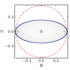
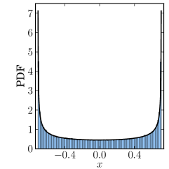
If the matrix A𝐴A is non–normal the numerical range forms an elliptical disk with λ1,λ2subscript𝜆1subscript𝜆2\lambda_{1},\lambda_{2} as focal points and minor axis, d=TrAA|λ1|2|λ2|2𝑑Tr𝐴superscript𝐴superscriptsubscript𝜆12superscriptsubscript𝜆22d=\sqrt{{\rm Tr}AA^{*}-|\lambda_{1}|^{2}-|\lambda_{2}|^{2}}. For a simple proof of this 1932 result of Murnaghan [17] see the note by Li [18]. In this generic case the numerical shadow is given by the probability distribution obtained by the projection of the hollow Bloch sphere of one–qubit pure states onto a plane [13]. In particular, the cross–section of the numerical shadow supported in an interval x[0,1]𝑥01x\in[0,1] is given by the arcsine distribution, P(x)=1/(πx(1x))𝑃𝑥1𝜋𝑥1𝑥P(x)=1/(\pi\sqrt{x(1-x)}). Non-normal case is shown in Fig.1, obtained for a matrix,

A0(2)=a0[1101].subscriptsuperscript𝐴20subscript𝑎0delimited-[]1101A^{(2)}_{0}\ =\ a_{0}\left[\begin{array}[]{cc}1&1\\ 0&-1\end{array}\right]\ .

For simplicity we have selected the centred matrix such that TrA=0Tr𝐴0{\rm Tr}A=0 so that one has B=A𝐵𝐴B=A in eq. (17). The normalization constant a0=2/5subscript𝑎025a_{0}=\sqrt{2/5} is chosen in such a way that the scaling constant defining the projection in (18) is set to unity, α=1𝛼1\alpha=1, so the shadow of the set of quantum states is shown in its ’natural size’: The distance between both eigenvalues, l=2a1=2𝑙2subscript𝑎12l=2a_{1}=\sqrt{2}, is equal to the diameter of the Bloch ball, 2R2=22subscript𝑅222R_{2}=\sqrt{2}.

Refer to caption
(a) Shadow of matrix A0(2)subscriptsuperscript𝐴20A^{(2)}_{0}
Refer to caption
(b) Cross-section for =00\Im=0
Figure 1: Projection of the set Ω2subscriptΩ2\Omega_{2} of one–qubit states generated by the numerical shadows of operators of order N=2𝑁2N=2 a) numerical shadow of generic matrix A0(2)subscriptsuperscript𝐴20A^{(2)}_{0} with an elliptical support. Eigenvalues are denoted with crosses and dashed circle of radius R2=2/2subscript𝑅222R_{2}=\sqrt{2}/2 denotes the diameter of the Bloch ball. Numerically obtained histogram is plotted in black, analytical plot is blue. Plot is done for matrix translated in such a way that its trace ()(\star) is equal to zero and suitably rescaled. b) Histogram of cross-section of the shadow supported in the interval [12,12],1212\left[-\frac{1}{\sqrt{2}},\frac{1}{\sqrt{2}}\right], solid line represents a probability density function of the arcsine distribution P(x)=(π12x2)1.𝑃𝑥superscript𝜋12superscript𝑥21P(x)=\left(\pi\sqrt{\frac{1}{2}-x^{2}}\right)^{-1}.

4.2 One–qutrit states, N=3𝑁3N=3

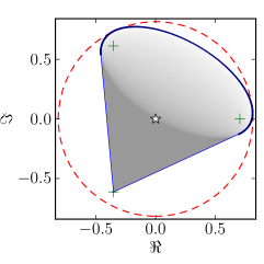
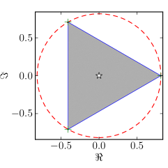
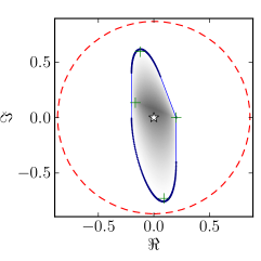
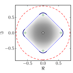
The structure of the numerical range for N=3𝑁3N=3 was analyzed in detail by Keeler et al. [19]. Numerical range of a matrix A𝐴A of order N=3𝑁3N=3 with spectrum λ1,λ2,λ3subscript𝜆1subscript𝜆2subscript𝜆3\lambda_{1},\lambda_{2},\lambda_{3} forms:

  1. a)

    a compact set of an ’ovular’ shape with three eigenvalues in its interior;

  2. b)

    a compact set with one flat part – e.g. the convex hull of a cardioid;

  3. c)

    a compact set with two flat parts – e.g. the convex hull of an ellipse and a point outside it;

  4. d)

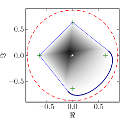
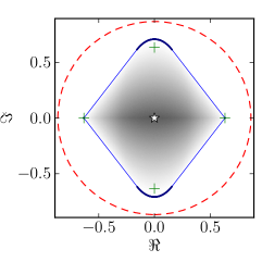
    triangle. For any normal matrix A𝐴A its numerical range is equal to the triangle spanned be the spectrum, W(A)=Δ(λ1,λ2,λ3)𝑊𝐴Δsubscript𝜆1subscript𝜆2subscript𝜆3W(A)=\Delta(\lambda_{1},\lambda_{2},\lambda_{3}). In the latter case the numerical shadow can be verbally interpreted as the shadow of the set 𝒞3subscript𝒞3{\cal C}_{3} of N=3𝑁3N=3 classical states – a uniformly covered equilateral triangle Δ2subscriptΔ2\Delta_{2}.

Refer to caption
(a) A0(3)subscriptsuperscript𝐴30A^{(3)}_{0}
Refer to caption
(b) A1(3)subscriptsuperscript𝐴31A^{(3)}_{1}
Refer to caption
(c) A2(3)subscriptsuperscript𝐴32A^{(3)}_{2}
Refer to caption
(d) A3(3)subscriptsuperscript𝐴33A^{(3)}_{3}
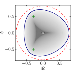
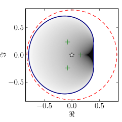
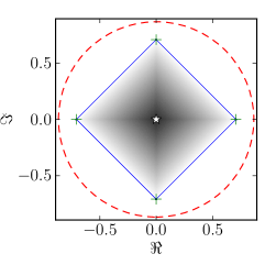
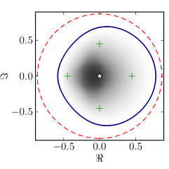
Figure 2: Projections of the set Ω3subscriptΩ3\Omega_{3} of one–qutrit states generated by the numerical shadows of operators of order N=3𝑁3N=3; a) a generic matrix A0(3)subscriptsuperscript𝐴30A^{(3)}_{0} with an oval–like numerical shadow, b) A1(3)subscriptsuperscript𝐴31A^{(3)}_{1} with one flat part of the boundary W𝑊\partial W of the numerical range, c) A2(3)subscriptsuperscript𝐴32A^{(3)}_{2} a simple sum with two flat parts of W𝑊\partial W, d) a diagonal normal matrix A3(3)subscriptsuperscript𝐴33A^{(3)}_{3} with numerical range equal to the triangle of eigenvalues, represented by (+)(+). Dashed circle of radius R3subscript𝑅3R_{3} represents projection of the sphere in which Ω3subscriptΩ3\Omega_{3} is inscribed. All plots are done for matrices translated in such a way that their trace ()(\star) is equal to zero and suitably rescaled.

The four classes of N=3𝑁3N=3 numerical ranges are illustrated in figure 2. It shows the numerical shadow supported on the corresponding numerical range, obtained for

A0(3)=a0[1110ω3100ω32],A1(3)=a1[53i0605+3i66610],formulae-sequencesubscriptsuperscript𝐴30subscript𝑎0delimited-[]1110subscript𝜔3100superscriptsubscript𝜔32subscriptsuperscript𝐴31subscript𝑎1delimited-[]53i06053i66610\displaystyle A^{(3)}_{0}=a_{0}\left[\begin{array}[]{ccc}1&1&1\\ 0&\omega_{3}&1\\ 0&0&\omega_{3}^{2}\end{array}\right],\ A^{(3)}_{1}=a_{1}\left[\begin{array}[]{ccc}5-3\mathrm{i}&0&6\\ 0&5+3\mathrm{i}&6\\ -6&-6&-10\end{array}\right],\
A2(3)=a2[1100ω3000ω32],A3(3)=a3[1000ω3000ω32].formulae-sequencesubscriptsuperscript𝐴32subscript𝑎2delimited-[]1100subscript𝜔3000superscriptsubscript𝜔32subscriptsuperscript𝐴33subscript𝑎3delimited-[]1000subscript𝜔3000superscriptsubscript𝜔32\displaystyle A^{(3)}_{2}=a_{2}\left[\begin{array}[]{ccc}1&1&0\\ 0&\omega_{3}&0\\ 0&0&\omega_{3}^{2}\end{array}\right],\ A^{(3)}_{3}=a_{3}\left[\begin{array}[]{ccc}1&0&0\\ 0&\omega_{3}&0\\ 0&0&\omega_{3}^{2}\end{array}\right].

The symbol ωksubscript𝜔𝑘\omega_{k} denotes the k𝑘k-th root of unity, so ω3=exp(i2π/3)subscript𝜔3i2𝜋3\omega_{3}=\exp(\mathrm{i}2\pi/3). As before the matrices are chosen to be traceless, so B=A𝐵𝐴B=A in (17) and the shadows are centered. Furthermore, the normalization constants are designed to assure that the scaling constant in eq. (18) in every case is set to unity, α=1𝛼1\alpha=1, so the Figure shows images of the set of quantum states in its natural size. For instance in the case of the diagonal matrix A3(3)subscriptsuperscript𝐴33A^{(3)}_{3} the prefactor reads a3=2/3subscript𝑎323a_{3}=\sqrt{2/3}, so that the eigenvalues are located at the distance 2/323\sqrt{2/3} from the origin. This is just the radius R3subscript𝑅3R_{3} of the sphere in which the set 𝒬3subscript𝒬3{\cal Q}_{3} is inscribed.

The study of the geometry of the numerical range was initiated by Kippenhahn [20] and later developed by Fiedler [21]. In more recent papers [22, 23] the differential topology and projection aspects of numerical range were investigated. In particular it was shown [22] that the numerical range of a generic matrix A𝐴A of order three pertains to the class a) above, as the boundary of W(A)𝑊𝐴W(A) does not contain intervals. Critical lines inside the range, analysed in [22, 23] where shown to influence the structure of the numerical shadow [13]. Thus we may now relate the critical lines with the geometry of complex projective spaces projected onto a plane.

In the one–qutrit case N=3𝑁3N=3 obtained probability distributions can be interpreted as images of the set of pure states Ω3=P2subscriptΩ3superscript𝑃2\Omega_{3}={\mathbbm{C}}P^{2} on the plane. Although it is not so simple to imagine the structure of the complex projective space [24], some experience is gained by studying numerical shadows of various non-normal matrices of size 333.

4.3 Four–level systems, N=4𝑁4N=4

Various shapes of the numerical range for matrices of size N=4𝑁4N=4 correspond to various projections of the set 𝒬4subscript𝒬4{\cal Q}_{4} of quantum states of size four. As in the case of the qutrit we analyse numerical shadows of traceless matrices normalized such that the scaling constant α𝛼\alpha is set to unity.

Even though several results on geometry of numerical range for N=4𝑁4N=4 are available [25, 26], complete classification of numerical ranges in this case is still missing. To provide an overview of the possible structure of the numerical shadow we analysed the following matrices of order four,
A0(4)=[11110i110011000i],subscriptsuperscript𝐴40delimited-[]11110𝑖110011000i\displaystyle A^{(4)}_{0}=\left[\begin{array}[]{cccc}1&1&1&1\\ 0&i&1&1\\ 0&0&-1&1\\ 0&0&0&-\mathrm{i}\end{array}\right], A1(4)=[i0100010111i00011],subscriptsuperscript𝐴41delimited-[]i0100010111i00011\displaystyle A^{(4)}_{1}=\left[\begin{array}[]{cccc}\mathrm{i}&0&-1&0\\ 0&0&-1&0\\ 1&1&1-\mathrm{i}&0\\ 0&0&1&1\end{array}\right], A2(4)=[10010i010010000i],subscriptsuperscript𝐴42delimited-[]10010i010010000i\displaystyle A^{(4)}_{2}=\left[\begin{array}[]{cccc}1&0&0&1\\ 0&\mathrm{i}&0&1\\ 0&0&-1&0\\ 0&0&0&-\mathrm{i}\end{array}\right],
A3(4)=[10010i100010000i],subscriptsuperscript𝐴43delimited-[]10010i100010000i\displaystyle A^{(4)}_{3}=\left[\begin{array}[]{cccc}1&0&0&1\\ 0&\mathrm{i}&1&0\\ 0&0&-1&0\\ 0&0&0&-\mathrm{i}\end{array}\right], A4(4)=[10010i000010000i],subscriptsuperscript𝐴44delimited-[]10010i000010000i\displaystyle A^{(4)}_{4}=\left[\begin{array}[]{cccc}1&0&0&1\\ 0&\mathrm{i}&0&0\\ 0&0&-1&0\\ 0&0&0&-\mathrm{i}\end{array}\right], A5(4)=[i0100010111i00001],subscriptsuperscript𝐴45delimited-[]i0100010111i00001\displaystyle A^{(4)}_{5}=\left[\begin{array}[]{cccc}\mathrm{i}&0&-1&0\\ 0&0&-1&0\\ 1&1&1-\mathrm{i}&0\\ 0&0&0&1\end{array}\right],
A6(4)=[10100i010010000i],subscriptsuperscript𝐴46delimited-[]10100i010010000i\displaystyle A^{(4)}_{6}=\left[\begin{array}[]{cccc}1&0&1&0\\ 0&\mathrm{i}&0&1\\ 0&0&-1&0\\ 0&0&0&-\mathrm{i}\end{array}\right], A7(4)=[10000i010010000i],subscriptsuperscript𝐴47delimited-[]10000i010010000i\displaystyle A^{(4)}_{7}=\left[\begin{array}[]{cccc}1&0&0&0\\ 0&\mathrm{i}&0&1\\ 0&0&-1&0\\ 0&0&0&-\mathrm{i}\end{array}\right], A8(4)=[10000i000010000i].subscriptsuperscript𝐴48delimited-[]10000i000010000i\displaystyle A^{(4)}_{8}=\left[\begin{array}[]{cccc}1&0&0&0\\ 0&\mathrm{i}&0&0\\ 0&0&-1&0\\ 0&0&0&-\mathrm{i}\end{array}\right].
Refer to caption
(a) A0(4)subscriptsuperscript𝐴40A^{(4)}_{0}
Refer to caption
(b) A1(4)subscriptsuperscript𝐴41A^{(4)}_{1}
Refer to caption
(c) A2(4)subscriptsuperscript𝐴42A^{(4)}_{2}
Refer to caption
(d) A3(4)subscriptsuperscript𝐴43A^{(4)}_{3}
Refer to caption
(e) A4(4)subscriptsuperscript𝐴44A^{(4)}_{4}
Refer to caption
(f) A5(4)subscriptsuperscript𝐴45A^{(4)}_{5}
Refer to caption
(g) A6(4)subscriptsuperscript𝐴46A^{(4)}_{6}
Refer to caption
(h) A7(4)subscriptsuperscript𝐴47A^{(4)}_{7}
Refer to caption
(i) A8(4)subscriptsuperscript𝐴48A^{(4)}_{8}
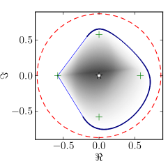
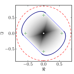
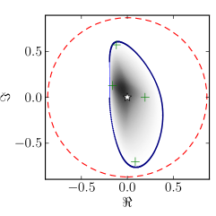
Figure 3: Projections of the set Ω4subscriptΩ4\Omega_{4} of N=4𝑁4N=4 quantum states emerging as numerical shadows of appropriately normalized operators of size 444: a) a generic matrix A0(4)subscriptsuperscript𝐴40A^{(4)}_{0} with a an oval–like numerical range W(A)𝑊𝐴W(A), b) A1(4)subscriptsuperscript𝐴41A^{(4)}_{1} with one flat part of the boundary W𝑊\partial W of the numerical range, c) A2(4)subscriptsuperscript𝐴42A^{(4)}_{2} being a simple sum 31direct-sum313\oplus 1 with two flat parts of W𝑊\partial W, d) A3(4)subscriptsuperscript𝐴43A^{(4)}_{3} – a simple sum 22direct-sum222\oplus 2 with two flat parts of W𝑊\partial W, e) A4(4)subscriptsuperscript𝐴44A^{(4)}_{4} three flat parts of W𝑊\partial W connected with corners and one oval–like part, f) A5(4)subscriptsuperscript𝐴45A^{(4)}_{5} three flat parts of W𝑊\partial W with only one corner and two oval–like parts, g) A6(4)subscriptsuperscript𝐴46A^{(4)}_{6} a simple sum 22direct-sum222\oplus 2, with four flat parts of W𝑊\partial W, h) A7(4)subscriptsuperscript𝐴47A^{(4)}_{7} pair of flat parts of W𝑊\partial W connected with a corner connected with two oval–like parts, i) a diagonal normal matrix A8(4)subscriptsuperscript𝐴48A^{(4)}_{8} with numerical range W𝑊W equal to the convex hull of eigenvalues denoted by (+)(+). All plots are done for matrices translated in such a way that their trace ()(\star) is equal to zero and suitably rescaled.

Numerical shadows of these representative of each class of N=4𝑁4N=4 matrices are shown in figure 3. The pictures can be interpreted as projections of the 666-dimensional complex projective space P3superscript𝑃3{\mathbbm{C}}P^{3} onto a plane. Making use of formula (18) we find that the normalization constant for the last example A8(4)subscriptsuperscript𝐴48A^{(4)}_{8} reads a8=1/2subscript𝑎812a_{8}=1/\sqrt{2}. Thus the diameter of the shadow, 2a4=22subscript𝑎422a_{4}=\sqrt{2}, coincides in this case with the Hilbert-Schmidt distance between any two orthogonal pure states in 𝒬4subscript𝒬4{\cal Q}_{4}. The dashed circle of radius R4=3/2subscript𝑅432R_{4}=\sqrt{3}/2 represents projection of the sphere into which the set 𝒬4subscript𝒬4{\cal Q}_{4} can be inscribed.

5 Unitary dynamics projected inside the numerical shadow

As the numerical range and the numerical shadow give us an opportunity to observe the structure of the space of quantum states, it is possible to apply these tools to investigate quantum dynamics. A unitary time evolution of a quantum system is governed by the Hamiltionian operator H𝐻H (i.e. a self-adjoint operator representing the total energy of the system), which leads to U(t)=exp(iHt)𝑈𝑡i𝐻𝑡U(t)=\exp(-\mathrm{i}Ht).

Note that eigenvalues of the Hamiltonian determine the cyclicity of the trajectory. The trajectory is periodic iff eigenvalues of the Hamiltonian are commensurable. The period in this case is given by least common multiple of the eigenvalues.

Let us consider a three-level system (qutrit). For concreteness, we choose the Hamiltionian

H=[11i11+i01+i11i1]𝐻delimited-[]11i11i01i11i1H=\left[\begin{array}[]{ccc}-1&-1-\mathrm{i}&1\\ -1+\mathrm{i}&0&1+\mathrm{i}\\ 1&1-\mathrm{i}&1\end{array}\right] (26)

and select an initial pure state of the system as |ψ(0)=|03ket𝜓0ket0subscript3|\psi(0)\rangle=|0\rangle\in{\cal H}_{3}. The state of the system at some specific time t𝑡t is described by the transformed state |ψ(t)=U(t)|ψ(0)ket𝜓𝑡𝑈𝑡ket𝜓0|\psi(t)\rangle=U(t)|\psi(0)\rangle.

Refer to caption
(a) A1subscript𝐴1A_{1}
Refer to caption
(b) A2subscript𝐴2A_{2}
Refer to caption
(c) A3subscript𝐴3A_{3}
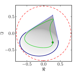
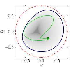
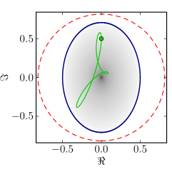
Figure 4: Shadow of the operators A1subscript𝐴1A_{1}, A2subscript𝐴2A_{2} and A3subscript𝐴3A_{3} of order three serves as a background for the trajectory representing the unitary dynamics defined by U=exp(iHt)𝑈i𝐻𝑡U=\exp(-\mathrm{i}Ht) with H𝐻H given by (26) with the initial state |ϕ(0)ketitalic-ϕ0|\phi(0)\rangle (marked by circle in the picture). All plots are done for matrices translated in such a way that their trace is equal to zero and suitably rescaled.

In order to use the numerical shadow to study the time evolution of the system, one needs to choose an arbitrary 3×3333\times 3 non-hermitian matrix. To get some information on the dynamics in the space of pure states of a qutrit and to observe it from different points of view, we selected the following matrices

A1=[0010i0001],A2=[0110i1001],A3=[i0200000i].formulae-sequencesubscript𝐴1delimited-[]0010i0001formulae-sequencesubscript𝐴2delimited-[]0110i1001subscript𝐴3delimited-[]i0200000iA_{1}=\left[\begin{array}[]{ccc}0&0&1\\ 0&\mathrm{i}&0\\ 0&0&-1\end{array}\right],A_{2}=\left[\begin{array}[]{ccc}0&1&1\\ 0&\mathrm{i}&1\\ 0&0&-1\end{array}\right],A_{3}=\left[\begin{array}[]{ccc}\mathrm{i}&0&2\\ 0&0&0\\ 0&0&-\mathrm{i}\end{array}\right]. (27)

For each of these auxiliary matrices, the quantum dynamics can be now visualized as a trajectory in the complex plane defined by a parametric equation,

z(t):=ψ(t)|A|ψ(t)=ψ(0)|A|ψ(0),assign𝑧𝑡quantum-operator-product𝜓𝑡𝐴𝜓𝑡quantum-operator-product𝜓0superscript𝐴𝜓0z(t):=\langle\psi(t)|A|\psi(t)\rangle=\langle\psi(0)|A^{\prime}|\psi(0)\rangle, (28)

where the unitarily transformed matrix reads A=UAU=eiHtAeiHtsuperscript𝐴superscript𝑈𝐴𝑈superscript𝑒i𝐻𝑡𝐴superscript𝑒i𝐻𝑡A^{\prime}=U^{*}AU=e^{\mathrm{i}Ht}Ae^{-\mathrm{i}Ht}. The time evolution of the initial state |ψ(0)=(1,0,0)T3ket𝜓0superscript100𝑇subscript3|\psi(0)\rangle=(1,0,0)^{T}\in{\cal H}_{3}. generated by the Hamiltonian (26) is shown in Fig. 4 from three different perspectives determined by matrices (27).

5.1 Identical trajectories

For given matrix A𝐴A and hermitian matrix H𝐻H a unitary time evolution induces a path in the numerical range ΛAsubscriptΛ𝐴\Lambda_{A} given by

ξeiHtAeiHtξ,forgivenstartingpointξ.superscript𝜉superscript𝑒i𝐻𝑡𝐴superscript𝑒i𝐻𝑡𝜉forgivenstartingpoint𝜉\xi^{*}e^{-\mathrm{i}Ht}Ae^{\mathrm{i}Ht}\xi,\mathrm{\ for\ given\ starting\ point\ }\xi. (29)

In the mixed state scenario the trajectory is given by

trρeiHtAeiHt,forgivenstartingpointρ.trace𝜌superscript𝑒i𝐻𝑡𝐴superscript𝑒i𝐻𝑡forgivenstartingpoint𝜌\tr\rho e^{-\mathrm{i}Ht}Ae^{\mathrm{i}Ht},\mathrm{\ for\ given\ starting\ point\ }\rho. (30)

The question one may pose is: under what conditions for two different starting points ρ0subscript𝜌0\rho_{0} and ρ1subscript𝜌1\rho_{1} trajectories on numerical range of A𝐴A are identical:

trρ0eiHtAeiHt=trρ1eiHtAeiHt,t.formulae-sequencetracesubscript𝜌0superscript𝑒i𝐻𝑡𝐴superscript𝑒i𝐻𝑡tracesubscript𝜌1superscript𝑒i𝐻𝑡𝐴superscript𝑒i𝐻𝑡𝑡\tr\rho_{0}e^{-\mathrm{i}Ht}Ae^{\mathrm{i}Ht}=\tr\rho_{1}e^{-\mathrm{i}Ht}Ae^{\mathrm{i}Ht},\ t\in\mathbb{R}. (31)

To convince yourself that such a situation may occur consider the daily rotation of the earth around its axis. Choosing two initial points at the same meridian on opposite sides of the equator (say close to Cairo and Durban in Africa), we see that the trajectories they generate after projecting onto the equatorial plane do coincide. This is because the dynamics, both initial points and the kind of the projection, are chosen in a special way and satisfy certain constraints. To characterize these constrains in a general setting we start with the following definitions.

For given matrix A𝐴A, let XA={BMNH():trB=0,trBA=0}subscript𝑋𝐴conditional-set𝐵superscriptsubscript𝑀𝑁𝐻formulae-sequencetrace𝐵0trace𝐵𝐴0X_{A}=\{B\in M_{N}^{H}(\mathbb{C}):\tr B=0,\ \tr BA=0\}. We also define the set HAsubscript𝐻𝐴H_{A}

HA={HMNH():t>0,BXAwehaveAdeiHt(B)XA},subscript𝐻𝐴conditional-set𝐻superscriptsubscript𝑀𝑁𝐻formulae-sequencefor-all𝑡0𝐵subscript𝑋𝐴wehavesubscriptAdsuperscript𝑒i𝐻𝑡𝐵subscript𝑋𝐴H_{A}=\{H\in M_{N}^{H}(\mathbb{C}):\forall t>0,B\in X_{A}\mathrm{\ we\ have}\ \mathrm{Ad}_{e^{\mathrm{i}Ht}}(B)\in X_{A}\}, (32)

where AdAd\mathrm{Ad} is the adjoint mapping given by AdC(B)=CBC1subscriptAd𝐶𝐵𝐶𝐵superscript𝐶1\mathrm{Ad}_{C}(B)=CBC^{-1}.

Now we can state fact concerning identical trajectories.

Lemma 7

Trajectories trρ0eiHtAeiHttracesubscript𝜌0superscript𝑒i𝐻𝑡𝐴superscript𝑒i𝐻𝑡\tr\rho_{0}e^{-\mathrm{i}Ht}Ae^{\mathrm{i}Ht} and trρ1eiHtAeiHttracesubscript𝜌1superscript𝑒i𝐻𝑡𝐴superscript𝑒i𝐻𝑡\tr\rho_{1}e^{-\mathrm{i}Ht}Ae^{\mathrm{i}Ht} for t𝑡t\in\mathbb{R} are identical if and only if ρ0ρ1XAsubscript𝜌0subscript𝜌1subscript𝑋𝐴\rho_{0}-\rho_{1}\in X_{A} and HHA𝐻subscript𝐻𝐴H\in H_{A}.

The definition of HAsubscript𝐻𝐴H_{A} is somehow complicated, here we put reasoning which presents it in a simpler form. We have following property AdC=eadCsubscriptAd𝐶superscript𝑒subscriptad𝐶\mathrm{Ad}_{C}=e^{\mathrm{ad}_{C}}, where adC(B)=[C,B]subscriptad𝐶𝐵𝐶𝐵\mathrm{ad}_{C}(B)=[C,B] (see e.g. [34]). Using above we can state the following lemma.

Lemma 8

Hermitian matrix H𝐻H is an element of HAsubscript𝐻𝐴H_{A}, if and only if, for all BXA𝐵subscript𝑋𝐴B\in X_{A} we have adiH(B)XAsubscriptadi𝐻𝐵subscript𝑋𝐴\mathrm{ad}_{\mathrm{i}H}(B)\in X_{A}.

Proof. If adiH(B)XAsubscriptadi𝐻𝐵subscript𝑋𝐴\mathrm{ad}_{\mathrm{i}H}(B)\in X_{A} for all BXA𝐵subscript𝑋𝐴B\in X_{A}, then by iterating we have that adiHk(B)XAsuperscriptsubscriptadi𝐻𝑘𝐵subscript𝑋𝐴\mathrm{ad}_{\mathrm{i}H}^{k}(B)\in X_{A} for k=0,1,𝑘01k=0,1,\dots. Since XAsubscript𝑋𝐴X_{A} is a linear space we obtain, that

AdeitH(B)=k=0tkk!adiHk(B)XA.subscriptAdsuperscript𝑒i𝑡𝐻𝐵superscriptsubscript𝑘0superscript𝑡𝑘𝑘superscriptsubscriptadi𝐻𝑘𝐵subscript𝑋𝐴\mathrm{Ad}_{e^{\mathrm{i}tH}}(B)=\sum_{k=0}^{\infty}\frac{t^{k}}{k!}\mathrm{ad}_{\mathrm{i}H}^{k}(B)\in X_{A}. (33)

On the other hand if AdeitH(B)XAsubscriptAdsuperscript𝑒i𝑡𝐻𝐵subscript𝑋𝐴\mathrm{Ad}_{e^{\mathrm{i}tH}}(B)\in X_{A}, then using the fact that

i[H,B]=limt0eiHtBeiHtBt,i𝐻𝐵subscript𝑡0superscript𝑒i𝐻𝑡𝐵superscript𝑒i𝐻𝑡𝐵𝑡\mathrm{i}[H,B]=\lim_{t\to 0}\frac{e^{\mathrm{i}Ht}Be^{-\mathrm{i}Ht}-B}{t}, (34)

and the continuity of the function XtrXAmaps-to𝑋trace𝑋𝐴X\mapsto\tr XA we obtain the result. \square

Note, that the condition i[H,B]XAi𝐻𝐵subscript𝑋𝐴\mathrm{i}[H,B]\in X_{A} can be stated as trH[A,B]=0trace𝐻𝐴𝐵0\tr H[A,B]=0, this follows from the cyclicity of trace. The linear space XAsubscript𝑋𝐴X_{A} is a real N21d(A)superscript𝑁21𝑑𝐴N^{2}-1-d(A) dimensional space, where d(A)=dim({(A),(A)})𝑑𝐴dimension𝐴𝐴d(A)=\dim(\{\Re(A),\Im(A)\}), where (A)=12(A+A)𝐴12𝐴superscript𝐴\Re(A)=\frac{1}{2}(A+A^{*}) and (A)=12i(AA)𝐴12i𝐴superscript𝐴\Im(A)=\frac{1}{2\mathrm{i}}(A-A^{*}). Thus in the generic case XAsubscript𝑋𝐴X_{A} has dimension N23superscript𝑁23N^{2}-3. The set HAsubscript𝐻𝐴H_{A} forms a real subspace of hermitian matrices orthogonal to sum of two real subspaces (adi(A)(XA)subscriptadi𝐴subscript𝑋𝐴\mathrm{ad}_{\mathrm{i}\Re(A)}(X_{A}) and adi(A)(XA))\mathrm{ad}_{\mathrm{i}\Im(A)}(X_{A}))),

HA=(adi(A)(XA)adi(A)(XA)),subscript𝐻𝐴superscriptsubscriptadi𝐴subscript𝑋𝐴subscriptadi𝐴subscript𝑋𝐴bottomH_{A}=(\mathrm{ad}_{\mathrm{i}\Re(A)}(X_{A})\cup\mathrm{ad}_{\mathrm{i}\Im(A)}(X_{A}))^{\bot}, (35)

where denotes the orthogonal component in the real space of hermitian matrices.

6 Mixed states numerical shadow

The standard numerical shadow (2) of matrix A𝐴A is defined by choosing randomly a pure state ρ=|ψψ|𝜌ket𝜓bra𝜓\rho=|\psi\rangle\langle\psi| with respect to the unitarily invariant, natural measure on the set of pure states, and taking the expectation value TrAρTr𝐴𝜌{\rm Tr}A\rho. However, one may also consider an expression analogous to (6) and use it with a different measure in the set 𝒬Nsubscript𝒬𝑁{\cal Q}_{N} of mixed states. More precisely, we introduce the mixed states numerical shadow of A𝐴A with respect to a measure μ𝜇\mu,

PAμ(z):=𝒬Ndμ(ρ)δ(zTrρA).assignsubscriptsuperscript𝑃𝜇𝐴𝑧subscriptsubscript𝒬𝑁differential-d𝜇𝜌𝛿𝑧Tr𝜌𝐴P^{\mu}_{A}(z):=\int_{{\cal Q}_{N}}{\rm d}\mu(\rho)\delta\Bigl{(}z-{\rm Tr}\rho A\Bigr{)}. (36)

The measure μ𝜇\mu defined on the set 𝒬Nsubscript𝒬𝑁{\cal Q}_{N} of mixed states of size N𝑁N is supposed to be unitarily invariant. For instance, we will use the family of induced measures μKsubscript𝜇𝐾\mu_{K} obtained by taking a random pure state |ξNKket𝜉tensor-productsubscript𝑁subscript𝐾|\xi\rangle\in{\cal H}_{N}\otimes{\cal H}_{K} and generating a mixed state by partial trace over the K𝐾K–dimensional subsystem, ρ=TrK|ξξ|𝜌subscriptTr𝐾ket𝜉bra𝜉\rho={\rm Tr}_{K}|\xi\rangle\langle\xi|. Since the pure states |ξket𝜉|\xi\rangle are generated randomly the unitary matrices determining the eigenvectors of ρ𝜌\rho are distributed according to the Haar measure on U(N)𝑈𝑁U(N). The probability distribution of the eigenvalues λisubscript𝜆𝑖\lambda_{i} of the random mixed state ρ𝜌\rho of size N𝑁N obtained in this way reads

PN,K(λ)=CN,Kδ(1i=1Nλi)i=1NλiKNi<j(λiλj)2.subscript𝑃𝑁𝐾𝜆subscript𝐶𝑁𝐾𝛿1superscriptsubscript𝑖1𝑁subscript𝜆𝑖superscriptsubscriptproduct𝑖1𝑁superscriptsubscript𝜆𝑖𝐾𝑁subscriptproduct𝑖𝑗superscriptsubscript𝜆𝑖subscript𝜆𝑗2P_{N,K}(\lambda)=C_{N,K}\;\delta\left(1-\sum_{i=1}^{N}\lambda_{i}\right)\;\prod_{i=1}^{N}\lambda_{i}^{K-N}\prod_{i<j}(\lambda_{i}-\lambda_{j})^{2}\;. (37)

It is assumed here that KN𝐾𝑁K\geq N and the normalization constants CN,Ksubscript𝐶𝑁𝐾C_{N,K} are given in [27]. In the symmetric case, K=N𝐾𝑁K=N, the above formula simplifies and the measure μNsubscript𝜇𝑁\mu_{N} coincides with the flat Hilbert–Schmidt measure, induced by the metric (4). In the opposite case K<N𝐾𝑁K<N, the joint probability density function is given by (37) with exchanged parameters NK𝑁𝐾N\leftrightarrow K.

Consider now a pure state |ξket𝜉|\xi\rangle on the bi-partite N×K𝑁𝐾N\times K system. It can be represented in its Schmidt decomposition [2],

|ξ=i=1min{N,K}λi|ei|fi,ket𝜉superscriptsubscript𝑖1𝑁𝐾tensor-productsubscript𝜆𝑖ketsubscript𝑒𝑖ketsubscript𝑓𝑖|\xi\rangle=\sum_{i=1}^{\min\{N,K\}}\sqrt{\lambda_{i}}\;|e_{i}\rangle\otimes|f_{i}\rangle, (38)

where {|ei}i=1Nsuperscriptsubscriptketsubscript𝑒𝑖𝑖1𝑁\{|e_{i}\rangle\}_{i=1}^{N} is an orthonormal basis in Nsubscript𝑁{\cal H}_{N} while {|fi}i=1Ksuperscriptsubscriptketsubscript𝑓𝑖𝑖1𝐾\{|f_{i}\rangle\}_{i=1}^{K} is an orthonormal basis of Ksubscript𝐾{\cal H}_{K}. Taking a partial trace of the projector |ξξ|ket𝜉bra𝜉|\xi\rangle\langle\xi| over the K𝐾K dimensional system we see that the spectrum of the resulting mixed state ρ𝜌\rho coincides with the set of the Schmidt coefficients {λi}subscript𝜆𝑖\{\lambda_{i}\} of the pure state |ξket𝜉|\xi\rangle. Thus formula (37) describes the distribution of the Schmidt coefficients of a pure state |ξket𝜉|\xi\rangle drawn randomly according to the uniform distribution on the sphere SNK1superscript𝑆𝑁𝐾1S^{NK-1}. By construction of the Schmidt decomposition of a random state |ξket𝜉|\xi\rangle, the vectors |eiketsubscript𝑒𝑖|e_{i}\rangle and |fiketsubscript𝑓𝑖|f_{i}\rangle can be considered as columns of unitary matrix in U(N)𝑈𝑁U(N) and U(K)𝑈𝐾U(K) respectively, distributed according to the Haar measure on the unitary group. A simple calculation shows that

ξ|(A𝟙K)|ξquantum-operator-product𝜉tensor-product𝐴subscript1𝐾𝜉\displaystyle\langle\xi|(A\otimes{\mathbbm{1}}_{K})|\xi\rangle =\displaystyle= i,j=1min{N,K}λiλjei|A|ejfi|fjsuperscriptsubscript𝑖𝑗1𝑁𝐾subscript𝜆𝑖subscript𝜆𝑗quantum-operator-productsubscript𝑒𝑖𝐴subscript𝑒𝑗inner-productsubscript𝑓𝑖subscript𝑓𝑗\displaystyle\sum_{i,j=1}^{\min\{N,K\}}\sqrt{\lambda_{i}\lambda_{j}}\langle e_{i}|A|e_{j}\rangle\langle f_{i}|f_{j}\rangle (39)
=\displaystyle= i=1min{N,K}λiei|A|ei=i=1min{N,K}λi(UAU)i,i,superscriptsubscript𝑖1𝑁𝐾subscript𝜆𝑖quantum-operator-productsubscript𝑒𝑖𝐴subscript𝑒𝑖superscriptsubscript𝑖1𝑁𝐾subscript𝜆𝑖subscriptsuperscript𝑈𝐴𝑈𝑖𝑖\displaystyle\sum_{i=1}^{\min\{N,K\}}\lambda_{i}\langle e_{i}|A|e_{i}\rangle=\sum_{i=1}^{\min\{N,K\}}\lambda_{i}(U^{\dagger}AU)_{i,i},

where U𝑈U is a unitary matrix distributed according to the Haar measure on U(N)𝑈𝑁U(N).

These considerations imply that the shadow of A𝟙Ktensor-product𝐴subscript1𝐾A\otimes\mathbbm{1}_{K} is a mixture of diagonal elements of A𝐴A in a random basis, given by the sum i=1min{N,K}λi(UAU)i,isuperscriptsubscript𝑖1𝑁𝐾subscript𝜆𝑖subscriptsuperscript𝑈𝐴𝑈𝑖𝑖\sum_{i=1}^{\min\{N,K\}}\lambda_{i}(U^{\dagger}AU)_{i,i}. As before U𝑈U stands for a random unitary matrix of size N𝑁N while the joint probability distribution function of the coefficients λisubscript𝜆𝑖\lambda_{i} is given by (37). This proves that the mixed states shadow of A𝐴A with respect to the induced measure μKsubscript𝜇𝐾\mu_{K} coincides with the standard numerical shadow of the extended operator A𝟙Ktensor-product𝐴subscript1𝐾A\otimes{\mathbbm{1}}_{K},

PAμK(z)=PA𝟙K(z)=P𝟙KA(z).subscriptsuperscript𝑃subscript𝜇𝐾𝐴𝑧subscript𝑃tensor-product𝐴subscript1𝐾𝑧subscript𝑃tensor-productsubscript1𝐾𝐴𝑧P^{\mu_{K}}_{A}(z)=P_{A\otimes{\mathbbm{1}}_{K}}(z)=P_{{\mathbbm{1}}_{K}\otimes A}(z). (40)

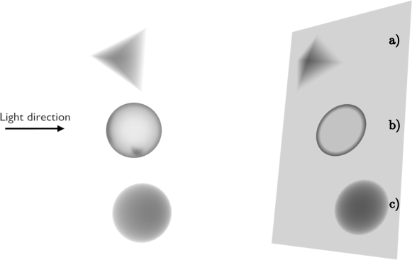
The last equality follows from the property (20). In the most important case, K=N𝐾𝑁K=N, the induced measure μNsubscript𝜇𝑁\mu_{N} is equivalent to the Euclidean (flat) measure in N21superscriptsuperscript𝑁21{\mathbbm{R}}^{N^{2}-1}, corresponding to the Hilbert-Schmidt distance (4). Thus the projection of the ’full’ set 𝒬Nsubscript𝒬𝑁{\cal Q}_{N} of mixed quantum states on the plane determined by a given matrix A𝐴A of size N𝑁N is equivalent to the standard shadow of an extended operator A𝟙Ntensor-product𝐴subscript1𝑁A\otimes{\mathbbm{1}}_{N}. In the case of N=2𝑁2N=2 this is visualized in figure 5c), in which the shadow of the full Bloch ball 𝒬2subscript𝒬2{\cal Q}_{2} can be compared with the shadow of the hollow Bloch sphere Ω2=S2subscriptΩ2superscript𝑆2\Omega_{2}=S^{2}, displayed in figure 5b).

Note that for K=1𝐾1K=1 the induced measure μ1subscript𝜇1\mu_{1} is supported on the set ΩNsubscriptΩ𝑁\Omega_{N} of pure states only and coincides with the Fubini–Study measure, so formula (36) with μ=μ1𝜇subscript𝜇1\mu=\mu_{1} reduces to the standard definition (2) of the pure states numerical shadow.
Refer to caption
Figure 5: Sketch of a projections onto a two-plane of a) the set 𝒞4=Δ3subscript𝒞4subscriptΔ3{\cal C}_{4}=\Delta_{3} of N=4𝑁4N=4 classical states onto the quadrangle formed by the numerical range W𝑊W of a normal matrix A𝐴A of order 444; b) the set Ω2=S2subscriptΩ2superscript𝑆2\Omega_{2}=S^{2} of one–qubit pure quantum states onto a disk formed by the numerical range of a non–normal Jordan matrix J2subscript𝐽2J_{2} of order 222; c) a mixed–states numerical shadow of J2subscript𝐽2J_{2}, corresponding to the projection of the full 333-dimensional Bloch ball onto a plane, is equal to the standard, pure states shadow of an extended matrix J2𝟙2tensor-productsubscript𝐽2subscript12J_{2}\otimes{\mathbbm{1}}_{2}. The picture is plotted using perspective.

7 Large N𝑁N limit and random matrices

It is instructive to analyse the numerical shadow of a random matrix in the limit of large matrix dimension N𝑁N. Let us consider two cases of the problem: the shadow of a random density matrix σ𝜎\sigma generated according to the induced measures [27] and the shadow of random unitary matrix U𝑈U distributed with respect to the Haar measure on U(N)𝑈𝑁U(N).

The numerical shadow of random matrix which is distributed with unitarily invariant measure is related to the distribution of its arbitrary diagonal element in a fixed basis. In this section we consider the measures induced by partial trace and the Haar measure on the unitary group, which are unitarily invariant. Let us start with the following

Lemma 9

Let A𝐴A be a random square matrix of order N𝑁N distributed according to a unitarily invariant measure. Let |xket𝑥|x\rangle be a random pure state of size N𝑁N generated according to the Fubini-Study measure on ΩN=PN1subscriptΩ𝑁superscript𝑃𝑁1\Omega_{N}={\mathbbm{C}}P^{N-1}. Then the expectation value has the same distribution as the matrix element A1,1subscript𝐴11A_{1,1}

P(x|A|x)=P(A1,1).𝑃quantum-operator-product𝑥𝐴𝑥𝑃subscript𝐴11P\left(\langle x|A|x\rangle\right)=P\left(A_{1,1}\right). (41)

Proof. Since |xket𝑥|x\rangle is a random pure state, thus |xU|0similar-toket𝑥𝑈ket0|x\rangle\sim U|0\rangle, where |0ket0|0\rangle is an arbitrary fixed state while U𝑈U is a random unitary matrix of size N𝑁N. Now we write

P(x|A|x)=P(0|UAU|0)=P(A1,1).𝑃quantum-operator-product𝑥𝐴𝑥𝑃quantum-operator-product0superscript𝑈𝐴𝑈0𝑃subscript𝐴11P\left(\langle x|A|x\rangle\right)=P\left(\langle 0|U^{\dagger}AU|0\rangle\right)=P\left(A_{1,1}\right). (42)

The last equality follows from invariance of the distribution P(A)𝑃𝐴P(A) with respect to unitary transformations.\square

7.1 Shadow of random quantum state

Consider a random density matrix σ𝜎\sigma of size N𝑁N generated with respect to the Hilbert-Schmidt measure μHSsubscript𝜇𝐻𝑆\mu_{HS}, so that its eigenvalues λisubscript𝜆𝑖\lambda_{i} are distributed according to eq. (37) with K=N𝐾𝑁K=N [27]. The diagonal elements of σ𝜎\sigma are of the form

σii=j=iN(ξij2+ηij2)j,k=1N(ξjk2+ηjk2),subscript𝜎𝑖𝑖superscriptsubscript𝑗𝑖𝑁superscriptsubscript𝜉𝑖𝑗2superscriptsubscript𝜂𝑖𝑗2superscriptsubscript𝑗𝑘1𝑁superscriptsubscript𝜉𝑗𝑘2superscriptsubscript𝜂𝑗𝑘2\sigma_{ii}=\frac{\sum_{j=i}^{N}(\xi_{ij}^{2}+\eta_{ij}^{2})}{\sum_{j,k=1}^{N}(\xi_{jk}^{2}+\eta_{jk}^{2})}, (43)

where ξijsubscript𝜉𝑖𝑗\xi_{ij} and ηijsubscript𝜂𝑖𝑗\eta_{ij} are independent, identically distributed random variables with normal distribution 𝒩(0,1)𝒩01\mathcal{N}(0,1). Basic properties of the Gamma distribution Γ(a,b)Γ𝑎𝑏\Gamma(a,b) [28] imply that

σii=G1G1+G2,subscript𝜎𝑖𝑖subscript𝐺1subscript𝐺1subscript𝐺2\sigma_{ii}=\frac{G_{1}}{G_{1}+G_{2}}, (44)

where G1subscript𝐺1G_{1} and G2subscript𝐺2G_{2} are stochastically independent variables distributed according to the Gamma distribution Γ(N,2)Γ𝑁2\Gamma(N,2) and Γ(N(N1),2)Γ𝑁𝑁12\Gamma(N(N-1),2) respectively. Therefore the diagonal elements of a random matrix σ𝜎\sigma generated according to the measure μHSsubscript𝜇𝐻𝑆\mu_{HS} are described by the Beta distribution with parameters {N,N(N1)}𝑁𝑁𝑁1\{N,N(N-1)\}.

The same reasoning can also be used for a general class of induced measures (37) parameterized by the size K𝐾K of the auxiliary subsystem. In this case the diagonal elements of a density matrix σ𝒬N𝜎subscript𝒬𝑁\sigma\in{\cal Q}_{N} generated with respect to the measure μN,Ksubscript𝜇𝑁𝐾\mu_{N,K} are distributed according to the Beta distribution with parameters {K,K(N1)}𝐾𝐾𝑁1\{K,K(N-1)\}.

Using the above reasoning and Lemma 9 we get the following

Lemma 10

The numerical shadow of a random matrix σ𝜎\sigma generated with respect to the induced measure μN,Ksubscript𝜇𝑁𝐾\mu_{N,K} is given by the Beta distribution with parameters {K,K(N1)}𝐾𝐾𝑁1\{K,K(N-1)\}, which can be expressed in terms of the Beta function,

Pσ(r)=1B(K,K(N1))(1r)K1rK(N1)1,0r1.formulae-sequencesubscript𝑃𝜎𝑟1𝐵𝐾𝐾𝑁1superscript1𝑟𝐾1superscript𝑟𝐾𝑁110𝑟1P_{\sigma}(r)=\frac{1}{B(K,K(N-1))}(1-r)^{K-1}r^{K(N-1)-1},\quad 0\leq r\leq 1. (45)

7.2 Random unitary matrices

Let us now consider a random unitary matrix U𝑈U distributed according to the Haar measure.

Lemma 11

The numerical shadow of a Haar random unitary matrix is supported in the unit disk. This distribution is invariant with respect to rotations, and |x|U|x|2superscriptquantum-operator-product𝑥𝑈𝑥2|\langle x|U|x\rangle|^{2} is distributed according to the Beta distribution with parameters {1,N1}1𝑁1\{1,N-1\}.

Proof. Random unitary matrix distributed with Haar measure can be generated using the QR decomposition of matrices pertaining to the Ginibre ensemble [29]. The QR factorization can be realized by a Gram-Schmidt orthogonalization procedure. Then the element U1,1subscript𝑈11U_{1,1} of the generated unitary matrix reads

U1,1=A1,1i=1N|Ai,1|2,subscript𝑈11subscript𝐴11superscriptsubscript𝑖1𝑁superscriptsubscript𝐴𝑖12U_{1,1}=\frac{A_{1,1}}{\sqrt{\sum_{i=1}^{N}|A_{i,1}|^{2}}}, (46)

where A𝐴A is a nonhermitian random matrix from the Ginibre ensemble. Therefore

|U1,1|2=ξ1,12+η1,12i=1N(ξi,12+ηi,12),superscriptsubscript𝑈112superscriptsubscript𝜉112superscriptsubscript𝜂112superscriptsubscript𝑖1𝑁superscriptsubscript𝜉𝑖12superscriptsubscript𝜂𝑖12|U_{1,1}|^{2}=\frac{\xi_{1,1}^{2}+\eta_{1,1}^{2}}{\sum_{i=1}^{N}(\xi_{i,1}^{2}+\eta_{i,1}^{2})}, (47)

where ξijsubscript𝜉𝑖𝑗\xi_{ij} and ηijsubscript𝜂𝑖𝑗\eta_{ij} are independent, identically distributed random variables with normal distribution 𝒩(0,1)𝒩01\mathcal{N}(0,1). Thus |U1,1|2superscriptsubscript𝑈112|U_{1,1}|^{2} has the Beta distribution with parameters {1,N1}1𝑁1\{1,N-1\} and using Lemma 9 we arrive at the desired result. \square

8 Concluding remarks

Our study may be briefly summarized by the following observation. The numerical shadow of a normal operator acting on Nsubscript𝑁{\cal H}_{N} reflects the structure of the set of (mixed) classical states, which belong to the probability simplex ΔN1subscriptΔ𝑁1\Delta_{N-1}, while investigation of numerical shadows of non–normal operators provides information about the set 𝒬Nsubscript𝒬𝑁{\cal Q}_{N} of quantum states of size N𝑁N.

In particular we have shown that the set of orthogonal projections of the set 𝒬Nsubscript𝒬𝑁{\cal Q}_{N} of density matrices onto a two–plane is equivalent, up to shift and rescaling, to the set of all possible numerical ranges W(A)𝑊𝐴W(A) of matrices of order N𝑁N. The numerical shadow of A𝐴A forms a probability distribution on the plane, supported in W(A)𝑊𝐴W(A), which corresponds to the ’shadow’ of the complex projective space PN1superscript𝑃𝑁1{\mathbbm{C}}P^{N-1} covered uniformly according to the Fubini-Study measure, and projected onto the plane. Another probability distribution in W(A)𝑊𝐴W(A) is obtained if one projects onto this plane entire convex set 𝒬Nsubscript𝒬𝑁{\cal Q}_{N} of density matrices. If this set is covered uniformly with respect to the Hilbert-Schmidt (Euclidean) measure, an explicit expression for this distribution is derived. In this way the analysis of numerical ranges and numerical shadows of matrices of a fixed size N𝑁N contributes to our understanding of the intricate geometry of the set 𝒬Nsubscript𝒬𝑁{\cal Q}_{N} of quantum states [2].

The numerical range [30] and its generalizations [31, 16] found several application in various problems of quantum information theory. In analogy to the product numerical range, defined for spaces with a tensor product structure [32], one can introduce the numerical shadow restricted to the subset of separable (product) states or the set of maximally entangled states [12]. Analysing such restricted numerical shadows for operators of a composite dimension NM𝑁𝑀NM one may thus investigate the geometry of the selected set of separable (maximally entangled) quantum pure states. Such an approach is advocated in a forthcoming publication [33].

It is a pleasure to thank G. Auburn and S. Weis for fruitful discussions. Work by J. Holbrook was supported in part by an NSERC of Canada research grant. Work by P. Gawron and J.A. Miszczak was supported by the Polish Ministry of Science and Higher Education under the grant number N519 442339, Z. Puchała was supported by Polish Ministry of Science and Higher Education under the project number IP 2010 033 470, while K. Życzkowski acknowledges support by the Polish Ministry of Science and Higher Education grant number N202 090239. Authors would like to thank S. Opozda for his help with the preparation of 3D models.

References

  • [1] Mahler G and Weberruss V A 1995 Quantum Networks (Berlin: Springer)
  • [2] Bengtsson I and Życzkowski K 2006 Geometry of Quantum States (Cambridge: Cambridge University Press)
  • [3] Życzkowski K and Słomczyński W 2001 Monge metric on the sphere and geometry of quantum states J. Phys. A 34 6689-6722
  • [4] Kimura G 2003, Phys. Let. A 314 339
  • [5] Schirmer S G, Zhang T, Leahy J V 2004 Orbits of quantum states and geometry of Bloch vectors for N-level systems J. Phys. A 37 1389
  • [6] Jakóbczyk L and Siennicki M 2001 Phys. Lett. A 286 383
  • [7] Verstraete F, Dehaene J, De Moor B 2002 On the geometry of entangled states J. Mod. Opt. 49 1277
  • [8] Kimura G and Kossakowski A 2005 The Bloch-vector space for N–level systems Open Sys. Infor. Dyn. 12 207
  • [9] Weis S 2010 A note on touching cones and faces preprint arXiv:1010.2991
  • [10] Horn A and Johnson C R 1994 Topics in Matrix Analysis (Cambridge: Cambridge University Press)
  • [11] Gustafson K E and Rao D K M 1997 Numerical Range: The Field of Values of Linear Operators and Matrices (New York: Springer-Verlag)
  • [12] Życzkowski K, Choi M-D, Dunkl C, Holbrook J A, Gawron P, Miszczak J A, Puchała Z, Skowronek Ł 2009 Generalized numerical range as a versatile tool to study quantum entanglement, Oberwolfach Report 59 34–37
  • [13] Dunkl C. F., Gawron P, Holbrook J A, Puchała Z, Życzkowski K 2011 Numerical shadows: measures and densities on the numerical range Lin. Alg. Appl. 439 2042-2080
  • [14] Gallay T and Serre D 2011 The numerical measure of a complex matrix preprint arXiv:1009.1522
  • [15] Devroye L 1986 Non-Uniform Random Variate Generation (New York: Springer-Verlag)
  • [16] Gawron P, Puchała Z, Miszczak J A, Skowronek Ł, Życzkowski K 2010 Restricted numerical range: a versatile tool in the theory of quantum information J. Math. Phys. 51 102204
  • [17] Murnaghan F D 1932 On the field of values of a square matrix, Proc. Natl. Acad. Sci. 18 246-248
  • [18] Li C K 1996 A simple proof of the elliptical range theorem Proc. Am. Math. Soc. 124 1985-1986
  • [19] Keeler D S, Rodman L, Spitkovsky I M 1997 The numerical range of 3×3333\times 3 matrices, Lin. Alg. Appl. 252 115-1139
  • [20] Kippenhahn R 1951 Ueber den Wertevorrat einer Matrix Math. Nachricht. 6 193-228
  • [21] Fiedler M 1981 Geometry of the numerical range of matrices Lin. Alg. Appl. 37 81-96
  • [22] Jonckheere E, Ahmad F, Gutkin E 1998 Differential topology of numerical range Lin. Alg. Appl. 279 227–254
  • [23] Henrion D 2010 Semidefinite geometry of the numerical range E.J. Lin. Alg. 20 322-332
  • [24] Bengtsson I, Brännlund, K. Życzkowski K 2002 Pnsuperscript𝑃𝑛{\mathbbm{C}}P^{n}, or, entanglement illustrated Int. J. Mod. Phys. A17, 4675-4696
  • [25] Gau H–L 2006 Elliptic numerical ranges of 4×4444\times 4 matrices Taiwan. J. Math. 10 117-128
  • [26] Li H and Liu X 2009 Elliptic numerical ranges of 4×4444\times 4 matrices 2009 ETP International conference on Future Computer and Communication
  • [27] Życzkowski K and Sommers H-J 2001 Induced measures in the space of mixed quantum states J. Phys. A 34 7111-7125
  • [28] Feller W 1968 An Introduction to Probability Theory and Applications, Vol. 2 (New York: Wiley)
  • [29] Mezzadri F 2007 How to generate random matrices from the classical compact groups Notices AMS 54 592-604
  • [30] Kribs D W, Pasieka A, Laforest M, Ryan C, Silva M P 2009 Research problems on numerical ranges in quantum computing Lin. Mult. Algebra 57 491–502
  • [31] Schulte-Herbrüggen T, Dirr G, Helmke U, Glaser S J 2008 The significance of the C𝐶C-numerical range and the local c-numerical range in quantum control and quantum information Lin. Mult. Algebra 56 3-26
  • [32] Puchała Z, Gawron P, Miszczak J A, Skowronek Ł, Choi M-D, Życzkowski K 2010 Product numerical range in a space with tensor product structure Linear Algebra Applications 434 327-342
  • [33] Dunkl C F, Gawron P, Holbrook J A, Miszczak J A, Puchała Z, Życzkowski K 2011 Restricted numerical shadow and geometry of quantum entanglement, in preparation
  • [34] Hall B C 2003 Lie groups, Lie algebras, and representations: an elementary introduction (New York: Springer-Verlag)