Approximate deconvolution large eddy simulation
of a barotropic ocean circulation model

Abstract

This paper puts forth a new large eddy simulation closure modeling strategy for two-dimensional turbulent geophysical flows. This closure modeling approach utilizes approximate deconvolution, which is based solely on mathematical approximations and does not employ additional phenomenological arguments to the model. The new approximate deconvolution model is tested in the numerical simulation of the wind-driven circulation in a shallow ocean basin, a standard prototype of more realistic ocean dynamics. The model employs the barotropic vorticity equation driven by a symmetric double-gyre wind forcing, which yields a four-gyre circulation in the time mean. The approximate deconvolution model yields the correct four-gyre circulation structure predicted by a direct numerical simulation, on a coarser mesh but at a fraction of the computational cost. This first step in the numerical assessment of the new model shows that approximate deconvolution could represent a viable tool for under-resolved computations in the large eddy simulation of more realistic turbulent geophysical flows.

1 Introduction

As a first approximation, the mean near-surface currents in the oceans are driven by the mean effects of winds. Wind-driven flows of mid-latitude ocean basins have been studied by modelers using idealized single and double-gyre wind forcing. This type of double-gyre circulation characterizes all mid-latitude ocean basins, including those in the North and South Atlantic, as well as the North and South Pacific. The barotropic vorticity equation (BVE) represents one of the most commonly used mathematical models for this type of geostrophic flows with various dissipative and forcing terms (Majda and Wang, 2006). For more details on the physical mechanism and formulations of the BVE, the reader is referred to Holland and Rhines (1980); Munk and Wunsch (1982); Griffa and Salmon (1989); Cummins (1992); Greatbatch and Nadiga (2000); Nadiga and Margolin (2001); Fox-Kemper (2005); Cushman-Roisin (1994).

The main assumptions that go into the BVE model are hydrostatic balance, the $\beta$-plane approximation, geostrophic balance, and horizontal eddy viscosity parametrization. Despite the fact that the BVE models are a simplified version of the full-fledged equations of geophysical flows, their numerical simulation is still computationally challenging when long-time integration is required, as is the case in climate modeling. Thus, to further reduce the computational cost of the BVE, large eddy simulation (LES) appears to be a natural approach. In LES only the large spatial structures are approximated, whereas the small scales are modeled. This allows for much coarser spatial meshes and thus a computational cost that is significantly lower than that of a direct numerical simulation (DNS). To achieve the same order of physical accuracy as DNS, however, LES needs to correctly treat the closure problem (Meneveau and Katz, 2000; Sagaut, 2006; Berselli et al., 2006): the effect of the small scales on the large ones needs to be modeled. This closure problem represents a significant challenge for quasi-two-dimensional turbulent flows, such as those in the ocean and atmosphere (McWilliams, 1989; Danilov and Gurarie, 2000; Smith et al., 2002; Lesieur, 2008; Salmon, 1998; Majda, 2003; Holton, 2004; McWilliams, 2006; Vallis, 2006).

Two-dimensional turbulence is a fundamental topic for understanding of geophysical flows and behaves in a profoundly different way from the three-dimensional turbulence due to different energy cascade behavior (Kraichnan, 1967; Batchelor, 1969; Leith, 1971), which is described in the Kraichnan-Batchelor-Leith two-dimensional turbulence theory. In three-dimensional turbulence, energy is transferred forward, from large scales to smaller scales, via vortex stretching. In two dimensions that mechanism is absent, and under most forcing and dissipation conditions energy is transferred from smaller scales to larger scales, largely because of the potential enstrophy, a quadratic invariant defined as the integral of the square of the potential vorticity. The physical mechanism behind the enstrophy cascade is the stretching of small-scale vorticity gradients by the strain arising from larger-scale vortices (Chen et al., 2003). This results in energy being trapped at large scales in forced-dissipative two-dimensional flows. Additionally, enstrophy is transferred to the smaller scales from larger scales, and is finally dissipated at large wavenumbers. Danilov and Gurarie (2000) and Tabeling (2002) reviewed both theoretical and experimental two-dimensional turbulence studies and provided extensive insights into the applicability of two-dimensional turbulence theory to geophysical flows. We also refer the reader to the energy-enstrophy conservation arguments provided by Vallis (2006).

Modeling the ocean and atmosphere inspired the first LES models, but most of the subsequent development of LES has taken place in the engineering community (Sagaut, 2006; Berselli et al., 2006). The majority of LES models have been developed for three-dimensional turbulent flows, such as those encountered in engineering applications. These LES models fundamentally rely on the concept of the forward energy cascade and so their extension to geophysical flows is beset with difficulties. The effective viscosity values in oceanic models are much greater than the molecular viscosity of seawater, hence a uniform eddy viscosity coefficient is generally used to parameterize the unresolved, subfilter-scale effects in most oceanic models (McWilliams, 2006; Vallis, 2006). LES models specifically developed for two-dimensional turbulent flows, such as those in the ocean and atmosphere, are relatively scarce (Fox-Kemper and Menemenlis, 2008; Awad et al., 2009; Özgökmen et al., 2009; Chen et al., 2010), at least when compared to the plethora of LES models developed for three-dimensional turbulent flows. Holm and Nadiga (2003) combine the uniform eddy viscosity parametrization with the alpha regularization LES approach to capture the under-resolved flow where the grid length becomes greater than the specified Munk scale of the problem. In that work the structural alpha parameterization was tested on the BVE in an ocean basin with double-gyre wind forcing, which displays a four-gyre mean ocean circulation pattern. It was found that the alpha models provide a promising approach to LES closure modeling of the barotropic ocean circulation by predicting the correct four-gyre circulation structure for under-resolved flows.

This paper puts forth a new LES closure modeling strategy for two-dimensional turbulent geophysical flows. The new closure modeling approach utilizes approximate deconvolution (AD), which is particularly appealing for geophysical flows because of no additional phenomenological approximations to the BVE. The AD approach can achieve high accuracy by employing repeated filtering, which is computationally efficient and easy to implement. The AD method has been used successfully in LES of three-dimensional turbulent engineering flows (Stolz and Adams, 1999; Stolz et al., 2001a, b, 2004). We emphasize, however, that to the best of our knowledge, this is the first time that the AD methodology is used in LES of large scale geophysical flows, such as the barotropic ocean circulation flow we consider in this paper. To assess the new AD closure modeling approach, we test it on the same two-dimensional barotropic flow problem as that employed in Nadiga and Margolin (2001) and in Holm and Nadiga (2003).

The rest of the paper is organized as follows: The BVE, the mathematical model used in this report, is presented in Section 2. Section 3 presents the AD methodology and introduces the new closure model. The numerical methods used in our simulations are briefly discussed in Section 4. The results for the new AD model are presented in Section 5. Finally, the conclusions are summarized in Section 6.

2 Barotropic Vorticity Equation

In this section, we present the BVE, the mathematical model used in the numerical investigation of the new AD model. The BVE is one of the most used mathematical models for geostrophic flows with various dissipative and forcing terms (Majda and Wang, 2006). Studies of wind-driven circulation using an idealized double-gyre wind forcing have played an important role in understanding various aspects of ocean dynamics, including the role of mesoscale eddies and their effect on mean circulation. Following Greatbatch and Nadiga (2000), we briefly describe the BVE. For more details on the physical mechanism and various formulations utilized, the reader is referred to Holland and Rhines (1980); Munk and Wunsch (1982); Griffa and Salmon (1989); Cummins (1992); Greatbatch and Nadiga (2000); Nadiga and Margolin (2001); Fox-Kemper (2005).

The governing equations for two-dimensional incompressible barotropic flows can be written in dimensionless form of the potential vorticity formulation in the beta plane as the BVE:

$$\frac{\partial q}{\partial t}+J=D+F.$$ (1)

In Eq. (1), $q$ is the potential vorticity, defined as

$$q=\mbox{Ro}\,\omega+y,$$ (2)

where $\omega$ is the vorticity and Ro is the Rossby number.

The nonlinear convection term in Eq. (1), called the Jacobian, is defined as

$$J=\frac{\partial\psi}{\partial y}\frac{\partial q}{\partial x}-\frac{\partial\psi}{\partial x}\frac{\partial q}{\partial y},$$ (3)

where $\psi$ is the streamfunction. The kinematic relationship between the vorticity and the streamfunction yields the following Poisson equation:

$$\frac{\partial^{2}\psi}{\partial x^{2}}+\frac{\partial^{2}\psi}{\partial y^{2}}=-\omega.$$ (4)

The viscous dissipation in Eq. (1) has the form

$$D=\left(\frac{\delta_{M}}{L}\right)^{3}\left(\frac{\partial^{2}\omega}{\partial x^{2}}+\frac{\partial^{2}\omega}{\partial y^{2}}\right),$$ (5)

where $\delta_{M}$ is the Munk scale and $L$ is the basin dimension. The double-gyre wind forcing is given by

$$F=F_{0}\sin(\pi y),$$ (6)

where $F_{0}=1$ due to the Sverdrup velocity scale used for nondimensionalization (Greatbatch and Nadiga, 2000). In this nondimensionalization, the velocity scale is

$$V=\frac{\pi\ \tau_{0}}{\rho H\beta L},$$ (7)

where $\tau_{0}$ is the maximum amplitude of double-gyre wind stress, $\rho$ is the mean density, $H$ is the mean depth of the basin, and $\beta$ is the gradient of the Coriolis parameter at the basin center ($y=0$). The dimensionless variables are then defined as

$$x=\frac{\tilde{x}}{L},\ y=\frac{\tilde{y}}{L},\ t=\frac{\tilde{t}}{L/V},\ q=\frac{\tilde{q}}{\beta L},\ \psi=\frac{\tilde{\psi}}{VL},$$ (8)

where the tilde denotes the corresponding dimensional variables. In dimensionless form, there are only two physical parameters, the Rhines scale and the Munk scale, which are related to the physical parameters in the following way:

$$\frac{\delta_{I}}{L}=\left(\frac{V}{\beta L^{2}}\right)^{1/2};\quad\quad\frac{\delta_{M}}{L}=\left(\frac{\nu}{\beta L^{3}}\right)^{1/3},$$ (9)

where $\nu$ is the uniform eddy viscosity coefficient. The physical parameters in the BVE (1), the Rhines scale $\delta_{I}$ and the Munk scale $\delta_{M}$, are related to the Reynolds and Rossby numbers through the following formulas:

$$\frac{\delta_{I}}{L}=(\mbox{Ro})^{1/2},$$ (10)

$$\frac{\delta_{M}}{L}=(\mbox{Re}^{-1}\mbox{Ro})^{1/3},$$ (11)

where Re is the Reynolds number based on the basin dimension, $L$. We note that some authors use a boundary layer Reynolds number, which is written as

$$\mbox{Re}_{B}=\mbox{Re}\frac{\delta_{I}}{L}=\frac{\delta_{I}^{3}}{\delta_{M}^{3}},$$ (12)

where $\mbox{Re}_{B}\sim O(10)-O(10^{3})$ for oceanic flows (Fox-Kemper, 2005). Finally, in order to completely specify the mathematical model, boundary and initial conditions need to be prescribed. In many theoretical studies of large scale ocean circulation, slip or no-slip boundary conditions are used. Following these studies (e.g., Greatbatch and Nadiga, 2000; Nadiga and Margolin, 2001; Holm and Nadiga, 2003; Cummins, 1992; Özgökmen and Chassignet, 1998; Munk, 1950; Bryan, 1963), we use slip boundary conditions for the velocity, which translate into homogenous Dirichlet boundary conditions for the vorticity: $\omega|_{\Omega}=0$. The impermeability boundary condition is imposed as $\psi|_{\Omega}=0$. For the initial condition, we start our computations from a quiescent state ($q=0$) and integrate Eq. (1) until a statistically steady state is obtained in which the wind forcing, dissipation, and Jacobian balance each other.

3 Approximate Deconvolution Model

The AD approach aims to obtain accurate and stable approximations of the original, unfiltered flow variables when approximations of the filtered variables are available (Stolz and Adams, 1999; Germano, 2009). The AD methodology was developed in the image processing community, and has been successfully adapted to the closure problem in turbulence modeling for engineering flows (Stolz et al., 2001a, b; Adams and Stolz, 2002; Stolz et al., 2004). We emphasize that this approach is purely mathematical, with no additional phenomenological arguments being used. This is particularly appealing for LES of geophysical flows in which different energy transfer characteristics are displayed than those in three-dimensional turbulent flows, for which successful phenomenological modeling has been done. Next, we present the mathematical derivation of the new AD model for the BVE (1).

To derive the equations for the filtered flow variables, the BVE (1) is first filtered with a rapidly decaying spatial filter (to be specified later). Thus, using a bar to denote the filtered quantities, the filtered BVE reads:

$$\frac{\partial\bar{q}}{\partial t}+J(\bar{q},\bar{\psi})=\bar{D}+\bar{F}+S,$$ (13)

where $S$ is the subfilter-scale term, given by

$$S=-\overline{J(q,\psi)}+J(\bar{q},\bar{\psi}).$$ (14)

It is precisely at this point in the LES model derivation that the celebrated closure problem must be addressed. In order to close the filtered BVE (13), the subfilter-scale term $S$ in Eq. (14) needs to be modeled in terms of the filtered flow variables, $\bar{q}$ and $\bar{\psi}$.

This paper proposes a new LES closure modeling approach for two-dimensional turbulent geophysical flows. The AD approach can achieve high accuracy, is computationally efficient, and is easy to implement. Although the AD methodology has already been successfully used in LES of three-dimensional turbulent engineering flows (Stolz and Adams, 1999; Stolz et al., 2001a, b, 2004), this is the first time that it is used in LES of large scale geophysical flows, such as the barotropic ocean circulation flow considered in this paper.

The goal in AD is to use repeated filtering in order to obtain approximations of the unfiltered flow variables when approximations of the filtered flow variables are available. These approximations of the unfiltered flow variables are then used in the subfilter-scale terms to close the LES system. To derive the new AD model, we start by denoting by $G$ the spatial filtering operator: $Gq=\bar{q}$. Since $G=I-(I-G)$, an inverse to $G$ can be written formally as the non-convergent Neumann series:

$$G^{-1}\sim\sum_{i=1}^{\infty}(I-G)^{i-1}.$$ (15)

Truncating the series gives the van Cittert approximate deconvolution operator, $Q_{N}$. We truncate the series at $N$ and obtain $Q_{N}$ as an approximation of $G^{-1}$:

$$Q_{N}=\sum_{i=1}^{N}(I-G)^{i-1},$$ (16)

where $I$ is the identity operator. The approximations $Q_{N}$ are not convergent as $N$ goes to infinity, but rather are asymptotic as the filter radius, $\delta$, approaches zero (Berselli et al., 2006). An approximate deconvolution of $\bar{q}$ can now be obtained as follows:

$$q\approx q^{*}=Q_{N}\bar{q}.$$ (17)

For higher values of $N$ we get increasingly more accurate approximations of $q$:

$$Q_{1} = I$$ (18)

$$Q_{2} = 2I-G$$ (19)

$$Q_{3} = 3I-3G+G^{2}$$ (20)

$$Q_{4} = 4I-6G+4G^{2}-G^{3}$$ (21)

$$Q_{5} = 5I-10G+10G^{2}-5G^{3}+G^{4}$$ (22)

$$\vdots$$

Following the same approach as that used in Dunca and Epshteyn (2006), one can prove that these models are highly accurate ($O(\delta^{2N+2})$ modeling consistency error) and stable. We choose $N=5$ and find an AD approximation of the variable $q$ as

$$q\approx q^{*}=5\bar{q}-10\bar{\bar{q}}+10\bar{\bar{\bar{q}}}-5\bar{\bar{\bar{\bar{q}}}}+\bar{\bar{\bar{\bar{\bar{q}}}}}$$ (23)

and, similarly, an AD approximation of the variable $\psi$:

$$\psi\approx\psi^{*}=5\bar{\psi}-10\bar{\bar{\psi}}+10\bar{\bar{\bar{\psi}}}-5\bar{\bar{\bar{\bar{\psi}}}}+\bar{\bar{\bar{\bar{\bar{\psi}}}}}.$$ (24)

Using (23) and (24), we can now approximate the nonlinear Jacobian:

$$\overline{J(q,\psi)}\approx\overline{J(q^{*},\psi^{*})}.$$ (25)

Finally, using the approximation Eq. (25) in Eq. (14), closes the filtered BVE (13) and yields the new AD model:

$$\frac{\partial\bar{q}}{\partial t}+J(\bar{q},\bar{\psi})=\bar{D}+\bar{F}+S^{*},$$ (26)

where $S^{*}$ is the subfilter-scale term, given by

$$S^{*}=-\overline{J(q^{*},\psi^{*})}+J(\bar{q},\bar{\psi}).$$ (27)

To completely specify the new AD model (26)-(27), we need to choose a computationally efficient filtering operator. Following Stolz and Adams (1999), we use the following second-order accurate filtering operator:

$$\alpha\bar{f}_{i-1}+\bar{f}_{i}+\alpha\bar{f}_{i+1}=\left(\frac{1}{2}+\alpha\right)\left(f_{i}+\frac{f_{i-1}+f_{i+1}}{2}\right),$$ (28)

where the subscript $i$ is the spatial index in the $x$-direction. This results in a tridiagonal system of equations for each fixed value of $y$. A generalization of Eq. (28), the spectral-type high-order compact filter introduced in Visbal and Gaitonde (2002), is given by

$$\alpha\bar{f}_{i-1}+\bar{f}_{i}+\alpha\bar{f}_{i+1}=\sum_{n=0}^{M}\frac{a_{n}}{2}(f_{i+n}+f_{i-n}),$$ (29)

where $f$ is the computed value, and $\bar{f}$ is the corresponding once filtered value. This filter provides $2M$th-order accurate filtering on a $2M+1$ point stencil (Visbal and Gaitonde, 2002). The free parameter, $\alpha$, which is in the range $0\leq|\alpha|\leq 0.5$, determines the filtering properties, with high values of $\alpha$ yielding less dissipative results. The coefficients for different order filters are given in Table 1. In our numerical tests, we found that for moderately fine meshes, the range of $0.25\leq\alpha\leq 0.5$ is appropriate, but for coarser meshes, lower values (e.g., $\alpha=0.1$) should be used to eliminate spurious oscillations. Most of our numerical simulations use the free parameter $\alpha=0.25$ (Stolz and Adams, 1999). Since we used a second-order accurate space discretization in this study, the filtered simulations are conducted either by using the second-order accurate filter given in Eq. (28) or the fourth-order accurate compact filter given in Eq. (29) with different parameter values for $\alpha$.

	2nd-order	4th-order	6th-order	8th-order
$a_{0}$	$\frac{1}{2}+\alpha$	$\frac{5}{8}+\frac{3\alpha}{4}$	$\frac{11}{16}+\frac{5\alpha}{8}$	$\frac{93}{128}+\frac{70\alpha}{128}$
$a_{1}$	$\frac{1}{2}+\alpha$	$\frac{1}{2}+\alpha$	$\frac{15}{32}+\frac{17\alpha}{16}$	$\frac{7}{16}+\frac{18\alpha}{16}$
$a_{2}$	0	$-\frac{1}{8}+\frac{\alpha}{4}$	$-\frac{3}{16}+\frac{3\alpha}{8}$	$-\frac{7}{32}+\frac{14\alpha}{32}$
$a_{3}$	0	0	$\frac{1}{32}-\frac{\alpha}{16}$	$\frac{1}{16}-\frac{\alpha}{8}$
$a_{4}$	0	0	0	$-\frac{1}{128}+\frac{\alpha}{64}$

Table 1: Coefficients of the compact filters of various orders given by Eq. (29).

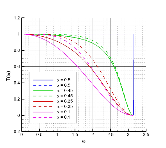
The existence and uniqueness of strong solutions of the BVE model using the AD closure was investigated by Stanculescu (2008). According to this work, the transfer function of the filter used in the AD closure should be positive definite. The transfer function of the tridiagonal filter given in Eq. (28) can be written as

$$T(\omega)=(\frac{1}{2}+\alpha)\frac{1+\cos(\omega)}{1+2\alpha\cos(\omega)}.$$ (30)

The transfer function of the generalized filter given in (29) can be written as

$$T(\omega)=\frac{\sum_{n=0}^{M}a_{n}\cos(n\ \omega)}{1+2\alpha\cos(\omega)}.$$ (31)

The transfer functions corresponding to the second- and fourth-order filters are plotted in Fig. (1) and are positive definite in the interval of $0\leq|\alpha|\leq 0.5$, where $\alpha$ is a free parameter of the filter. By substituting these transfer functions into the deconvolution operator, it can be easily seen that the transfer functions of the deconvolution operators also become positive definite. With these two conditions verified (the positive definiteness of the transfer functions of the filters and deconvolution operators), the theoretical results in Stanculescu (2008) provide solid mathematical support for our numerical investigations.

Figure 1: Transfer functions of the second-order (solid lines) and fourth-order (dashed lines) tridiagonal filters.

4 Numerical Methods

In this section, we provide a brief description of the numerical methods employed in the investigation of the new AD model. For the time discretization, we employ an optimal third-order total variation diminishing Runge-Kutta (TVDRK3) scheme (Gottlieb and Shu, 1998). For clarity of notation, we rewrite the new AD model in the following form

$$\frac{d\bar{q}}{dt}=R,$$ (32)

where $R$ denotes the discrete spatial derivative operator, including the nonlinear convective term, the linear diffusive term, the forcing term, and the subfilter-scale term. The TVDRK3 scheme then becomes

$$\bar{q}^{(1)} = \bar{q}^{n}+\Delta tR^{(n)}$$

$$\bar{q}^{(2)} = \frac{3}{4}\bar{q}^{n}+\frac{1}{4}\bar{q}^{(1)}+\frac{1}{4}\Delta tR^{(1)}$$ (33)

$$\bar{q}^{n+1} = \frac{1}{3}\bar{q}^{n}+\frac{2}{3}\bar{q}^{(2)}+\frac{2}{3}\Delta tR^{(2)},$$

where $\Delta t$ is the adaptive time step size which can be computed at the end of each time step by:

$$\Delta t=c\frac{\mbox{min}(\Delta x,\Delta y)}{\mbox{max}\left(|\frac{\partial\bar{\psi}}{\partial x}|,|\frac{\partial\bar{\psi}}{\partial y}|\right)},$$ (34)

where $c$ is known as Courant- Friedrichs -Lewy (CFL) number. We set $c=1.0$ for all the simulations reported here.

For the spatial discretization of linear operators, such as the viscous dissipation term and the Poisson equation, we use a second-order finite difference method. For the nonlinear convection term, we utilize Arakawa’s conservative scheme (Arakawa, 1966). Finally, a direct Poisson solver based on the fast sine transform is used to solve the kinematic relationship between the vorticity and the streamfunction in Eq. (4). Specifically, we use a fast sine transform in one direction and a tridiagonal system solver in the other direction (Moin, 2001).

For completeness, we summarize the solution algorithm for one time step. We assume that the numerical approximation for time level $n$ is known, and we seek the numerical approximation for time level $n+1$, after the time step $\Delta t$. We write the algorithm for the new AD model (26)-(27), but we emphasize that it is the same algorithm, with some obvious modifications, that is used for the high resolution well resolved simulation, which is referred to here as DNS. We emphasize that the term DNS in this study is not meant to indicate that a fully detailed solution is being computed, but instead refers to resolving the simulation down to the Munk scale via the specified lateral eddy viscosity parameterization. The solution algorithm has the following form

1. Compute $\bar{\psi}^{n}$ using the Poisson solver for the following equation:

   $$\frac{\partial^{2}\bar{\psi}^{n}}{\partial x^{2}}+\frac{\partial^{2}\bar{\psi}^{n}}{\partial y^{2}}=-\frac{1}{Ro}\left(\bar{q}^{n}-y\right).$$ (35)

2. Compute $q^{n*}$ and $\psi^{n*}$ using $\bar{q}^{n}$ and $\bar{\psi}^{n}$, the filtering procedure in Eq. (29), and the AD method in Eq. (23) and Eq. (24).

3. Compute the nonlinear Jacobian terms $\overline{J(q^{n*},\psi^{n*})}$ and $J(\bar{q}^{n},\bar{\psi}^{n})$ using the Arakawa scheme.

4. Compute the subfilter-scale term $S^{*}$ using $\overline{J(q^{n*},\psi^{n*})},J(\bar{q}^{n},\bar{\psi}^{n})$, and Eq. (27).

5. Compute the viscous dissipation term $\bar{D}$ using a central difference scheme and calculate the right-hand-side term $R$ in Eq. (32).

6. Apply the Runge-Kutta algorithm by repeating steps 1-5 for each stage of Runge-Kutta scheme.

7. Adjust the time step according to the CFL number given in Eq. (34).

8. Go to step 1 to begin the next time step.

5 Numerical Results

The main goal of this section is to test the new AD model (26)-(27) in the numerical simulation of the BVE (1). Before testing the new model, however, we first validate the code in Section 5.1. The new AD model is then tested in the numerical simulation of a four-gyre barotropic model with double-gyre wind forcing in Section 5.2.

5.1 Method of manufactured solutions: Code validation

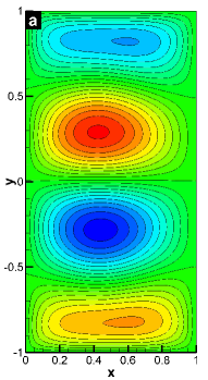
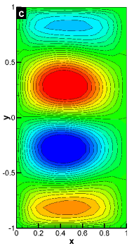
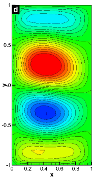
To validate the code, we consider the following exact solution, which corresponds to a steady state Taylor-Green vortex flow:

$$q(x,y,t) = \left(\frac{\delta_{I}}{L}\right)^{2}2\,\pi^{2}\sin(\pi x)\sin(\pi y)+y,$$ (36)

$$\omega(x,y,t) = 2\,\pi^{2}\sin(\pi x)\sin(\pi y),$$ (37)

$$\psi(x,y,t) = \sin(\pi x)\sin(\pi y).$$ (38)

The forcing function is calculated by plugging Eqs. (36)-(38) into the BVE (1):

$$F(x,y,t)=-\pi\,\cos(\pi x)\sin(\pi y)+\left(\frac{\delta_{M}}{L}\right)^{3}\,4\,\pi^{4}\sin(\pi x)\sin(\pi y).$$ (39)

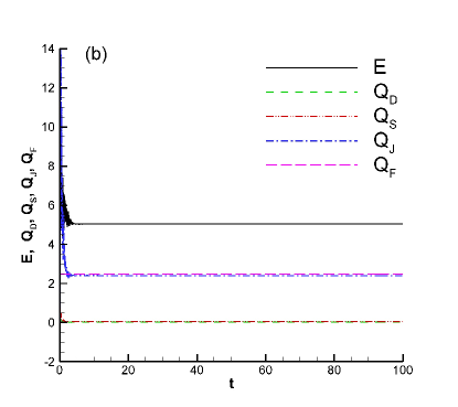
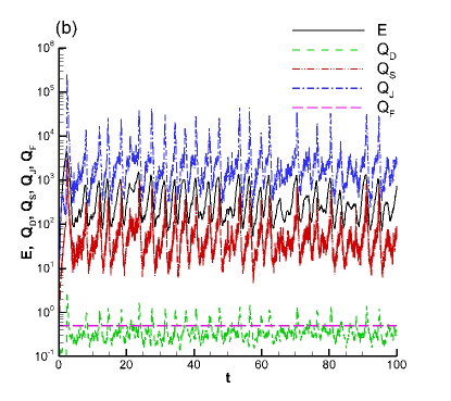
We use $q(x,y,0)=0$ as the initial condition. The spatial resolution is $64\times 128$ and the time step $\Delta t$ is computed adaptively as given in Eq. (34). We utilize the numerical algorithm in Section 4 to integrate the BVE until the steady state solution is obtained. Our numerical results closely match the exact solution. To investigate the individual effects of the nonlinear Jacobian, dissipation, forcing and subfilter-scale terms, we compute the time series of following integral quantities:

$$Q_{J}(t)=\frac{1}{2}\iint\left(J(\bar{q},\bar{\psi})\right)^{2}dx\,dy,$$ (40)

$$Q_{D}(t)=\frac{1}{2}\iint\bar{D}^{2}dx\,dy,$$ (41)

$$Q_{F}(t)=\frac{1}{2}\iint\bar{F}^{2}dx\,dy,$$ (42)

$$Q_{S}(t)=\frac{1}{2}\iint\left(S^{*}\right)^{2}dx\,dy.$$ (43)

We also plot with respect to time the total energy:

$$E(t)=\frac{1}{2}\iint\left(\frac{\partial\psi}{\partial y}\right)^{2}+\left(\frac{\partial\psi}{\partial x}\right)^{2}dx\,dy,$$ (44)

Since the exact steady state solution is given in Eqs. (36)-(38), we can calculate the exact values of the above integral quantities.

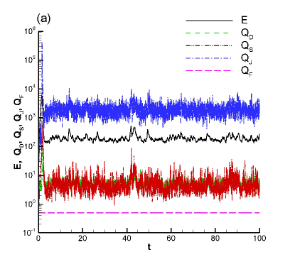
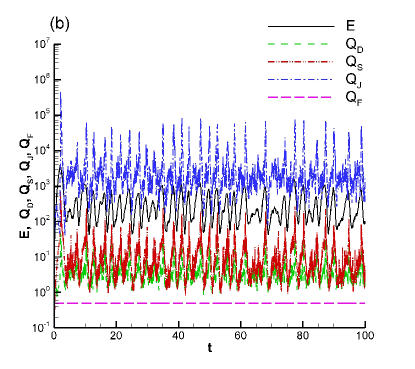
In Fig. (2) we plot the time evolution of the total energy, and contributions of the individual dissipation, subfilter-scale, nonlinear Jacobian, and forcing terms. We plot these time series for two parameter sets: $\displaystyle\delta_{I}/L=0.04$ and $\displaystyle\delta_{M}/L=0.02$ in Fig. (2a), and $\displaystyle\delta_{I}/L=0.06$ and $\displaystyle\delta_{M}/L=0.02$ in Fig. (2b). For both parameter sets, the time evolution of the above integral quantities follows the same pattern: after a short transient interval, they converge to the correct exact values. Thus, we conclude that the numerical algorithm produces accurate results for these validation test cases.

Figure 2: Code validation test case.Time history of the total energy, individual dissipation, Jacobian, subfilter-scale and forcing terms: (a) $\displaystyle\delta_{I}/L=0.04$ and $\displaystyle\delta_{M}/L=0.02$; and (b) $\displaystyle\delta_{I}/L=0.06$ and $\displaystyle\delta_{M}/L=0.02$. Note that the numerical approximation converges to the correct value after a short transient interval.

5.2 Four-gyre problem with double-gyre forcing

The main goal of this section is to test the new AD model Eqs. (26)-(27) in the numerical simulation of the wind-driven circulation in a shallow ocean basin, a standard prototype of more realistic ocean dynamics. The model employs the BVE driven by a symmetric double-gyre wind forcing, which yields a four-gyre circulation in the time mean. This test problem has been used in numerous studies (e.g., Cummins, 1992; Greatbatch and Nadiga, 2000; Nadiga and Margolin, 2001; Holm and Nadiga, 2003; Fox-Kemper, 2005). This problem represents an ideal test for the new AD model. Indeed, as showed in Greatbatch and Nadiga (2000), although a double gyre wind forcing is used, the long time average yields a four gyre pattern, which is challenging to capture on coarse spatial resolutions. Thus, we will investigate numerically whether the new AD model can reproduce the four gyre time average on a coarse mesh.

The mathematical model used in the four gyre problem is the BVE (1). The double-gyre forcing is given in Eq. (6). Following Holm and Nadiga (2003), we utilize two different parameter sets, corresponding to two physical oceanic settings: Experiment (i) with a Rhines scale of $\delta_{I}/L=0.04$ and a Munk scale of $\delta_{M}/L=0.02$, which corresponds to a Reynolds number of $Re=200$ (or a boundary layer based Reynolds number of $Re_{B}=8$) and a Rossby number of $Ro=0.0016$; and Experiment (ii) with a Rhines scale of $\delta_{I}/L=0.06$ and a Munk scale of $\delta_{M}/L=0.02$, which corresponds to a Reynolds number of $Re=450$ (or a boundary layer based Reynolds number of $Re_{B}=27$) and a Rossby number of $Ro=0.0036$. Since we set the Munk scale to $\delta_{M}/L=0.02$ in our study, the uniform eddy viscosity coefficient embedded in the model can be calculated from Eq. (9). For example, if we set the mid-latitude ocean basin length to $L=2000$ km and the gradient of the Coriolis parameter to $\beta=1.75\times 10^{-11}\ \mbox{m}^{-1}\mbox{s}^{-1}$, then our model uses $\nu=1120\ \mbox{m}^{2}\mbox{s}^{-1}$ as its eddy viscosity parametrization. All numerical experiments conducted here are solved for a maximum dimensionless time of $T_{max}=100$. This value corresponds to the dimensional times of $56.6$ and $25.15$ years for Experiment (i) and Experiment (ii), respectively, which are long enough to capture statistically steady states. All computations were carried out using the gfortran compiler on a Linux cluster system (3.4 GHz/node).

To assess the new AD model, we employ the standard LES methodology: we first run a DNS computation on a fine mesh. We then run an under-resolved numerical simulation on a much coarser mesh (denoted in what follows as BVE_coarse), which does not employ any subfilter-scale model. We expect BVE_coarse to produce inaccurate results. Finally, we employ the new AD model on the same coarse mesh utilized in BVE_coarse. The AD model should yield results that are significantly better than those obtained with BVE_coarse and are close to the DNS results, at a fraction of the computational cost.

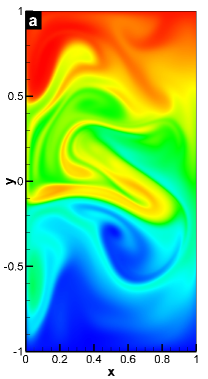
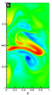
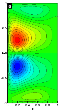
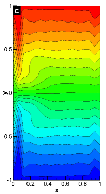
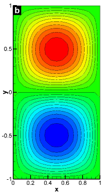
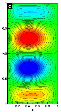
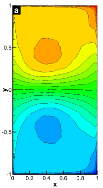
We start by performing a DNS computation on a fine mesh ($512\times 256$ spatial resolution). After a transient period, a statistically steady state solution is obtained at a time of around $t=10$. Instantaneous contour plots at time $t=90$ for the potential vorticity, vorticity, and streamfunction are shown in Fig. (3) and Fig. (4) for Experiment (i) and Experiment (ii), respectively. Two gyres are clearly seen in the streamfunction contour plots. Next, the time average of the data is taken between time $t=20$ and $t=100$ using $8001$ snapshots. The results are given in Fig. (5) and Fig. (6). We emphasize that, for both parameter sets, four gyres are clearly visible in the streamfunction plots. This is in stark contrast with the instantaneous streamfunction contour plots in Fig. (3) and Fig. (4), in which only two gyres are present. The computational time of each DNS run was longer than $3.5$ days.

Figure 3: Experiment (i):  DNS results for $Re=200,Ro=0.0016$ and a spatial resolution of $512\times 256$. Instantaneous field data for: (a) potential vorticity; (b) vorticity; and (c) streamfunction. Note that two gyres appear in the streamfunction contour plot.

Figure 4: Experiment (ii):  DNS results for $Re=450,Ro=0.0036$ and a spatial resolution of $512\times 256$. Instantaneous field data for: (a) potential vorticity; (b) vorticity; and (c) streamfunction. Note that two gyres appear in the streamfunction contour plot.

Figure 5: Experiment (i):  DNS results for $Re=200,Ro=0.0016$ and a spatial resolution of $512\times 256$. Time-averaged field data for: (a) potential vorticity; (b) vorticity; and (c) streamfunction. Note that four gyres appear in the streamfunction contour plot.

Figure 6: Experiment (ii):   DNS results for $Re=450,Ro=0.0036$ and a spatial resolution of $512\times 256$. Time-averaged field data for: (a) potential vorticity; (b) vorticity; and (c) streamfunction. Note that four gyres appear in the streamfunction contour plot.

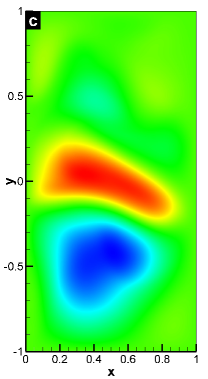
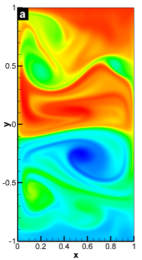
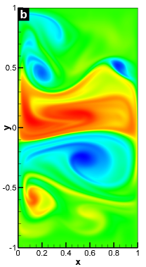
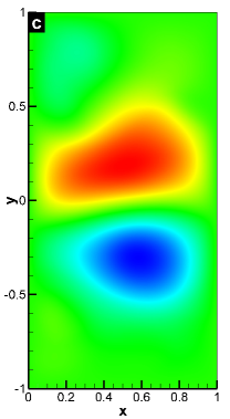
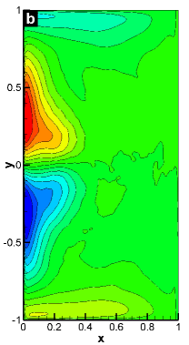
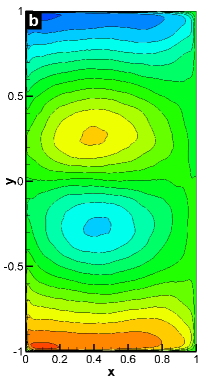
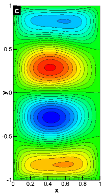
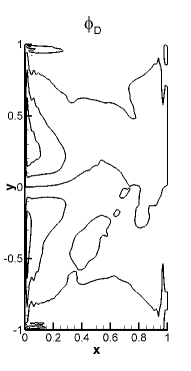
In addition to the time series of each individual term given by Eqs. (40)-(43), following Marshall and Pillar (2011), we compute the force functions in order to analyze the contribution of individual terms, including the subfilter-scale term, in the new AD model (26)-(27). The defining equations for the force functions corresponding to the dissipation, subfilter-scale, nonlinear Jacobian, and forcing terms are:

$$\nabla^{2}\phi_{D}=\bar{D},$$ (45)

$$\nabla^{2}\phi_{S}=S^{*},$$ (46)

$$\nabla^{2}\phi_{J}=\bar{J},$$ (47)

$$\nabla^{2}\phi_{F}=\bar{F}.$$ (48)

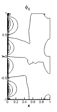
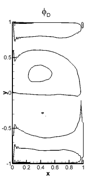
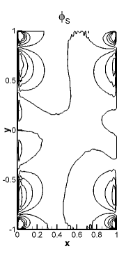
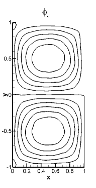
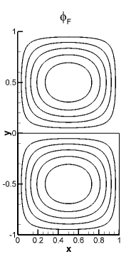
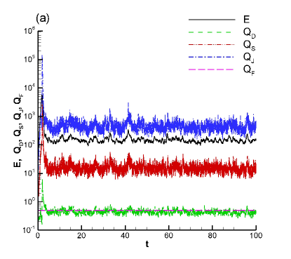
Solving these Poisson equations for time averaged data (between $t=20$ and $t=100$ using $8,001$ snapshots) yields the corresponding force functions. Fig. (7) and Fig. (8) illustrate these force function contour plots for Experiment (i) and Experiment (ii) for a spatial resolution of $128\times 64$. The time series of the total energy, dissipation, subfilter-scale, Jacobian and forcing terms are plotted in Fig. (9). It can be seen that at this spatial resolution the subfilter-scale effects are on the order of dissipation term.

Figure 7: Experiment (i):  AD results for $Re=200,Ro=0.0016$, and a spatial resolution of $128\times 64$. Time-averaged force function contour plots for the dissipation, subfilter-scale, Jacobian, and forcing terms. The contour intervals are between -0.05 and 0.05 for the forcing and Jacobian terms, and -0.002 and 0.002 for the dissipation and subfilter-scale terms.

Figure 8: Experiment (ii):   AD results for $Re=450,Ro=0.0036$, and a spatial resolution of $128\times 64$. Time-averaged force function contour plots for the dissipation, subfilter-scale, Jacobian, and forcing terms. The contour intervals are between -0.05 and 0.05 for the forcing and Jacobian terms, and -0.002 and 0.002 for the dissipation and subfilter-scale terms.

Figure 9: Time history of the total energy, dissipation, subfilter-scale, Jacobian, and forcing terms: (a) Experiment (i): $\displaystyle\delta_{I}/L=0.04$ and $\displaystyle\delta_{M}/L=0.02$; and (b) Experiment (ii): $\displaystyle\delta_{I}/L=0.06$ and $\displaystyle\delta_{M}/L=0.02$.

Next, we test the new AD model (26)-(27) using a coarser mesh with a spatial resolution of $32\times 16$, which is $16$ times coarser than the DNS mesh with a resolution of $512\times 256$. On this coarse mesh, we test both the new AD model and the under-resolved numerical simulation BVE_coarse, which does not employ any subfilter-scale model. To compare the models, we utilize data that is time-averaged between $t=20$ and $t=100$. The new AD model is tested with a second-order filtering operation and $N=5$ (as in Eq. (23) and Eq. (24)), and with the smoothing parameter $\alpha=0.25$.

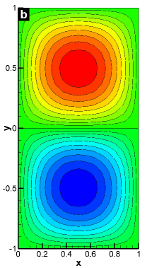
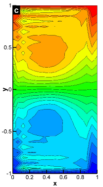
For $Re=200$ and $Ro=0.0016$ we plot the time-averaged streamfunction and potential vorticity contours in Fig. (10) and Fig. (11), respectively. We note that the new AD model yields improved results by smoothing out the numerical oscillations present in the under-resolved BVE_coarse results. This improvement is more clearly displayed in the potential vorticity contour plot in Fig. (11). For $Re=450$ and $Ro=0.0036$ we plot the time-averaged streamfunction and potential vorticity contours in Fig. (12) and Fig. (13), respectively. The new AD model yields results that are significantly better than those corresponding to the under-resolved BVE_coarse run. Indeed, in the streamfunction plot in Fig. (12) the new AD model clearly displays the correct four gyre pattern (as in the DNS plot), whereas the under-resolved BVE_coarse run incorrectly yields only two gyres, which is nonphysical. We also plot in Fig. (14) the time history of the total energy. It is clear that the new AD model yields accurate results that are close to the DNS results. The under-resolved BVE_coarse run, however, yields totally inaccurate results. The contributions of the individual terms in Experiment (i) and Experiment (ii), obtained using the AD model for under-resolved simulations at a spatial resolution of $32\times 16$, are also shown in Fig. (15). When we compare this to the higher resolution simulation illustrated in Fig. (9), it can be seen that the relative contribution of the subfilter-scale terms is more prominent in under-resolved simulations.

Figure 10: Experiment (i):   Time-averaged streamfunction data for $Re=200$ and $Ro=0.0016$: (a) DNS results at a resolution of $512\times 256$; (b) under-resolved BVE_coarse results at a resolution of $32\times 16$; (c) new AD model results at a resolution of $32\times 16$. Note the smoothing effect of the AD model on contour lines. Contour interval layouts are identical.

Figure 11: Experiment (i):   Time-averaged potential vorticity data for $Re=200$ and $Ro=0.0016$: (a) DNS results at a resolution of $512\times 256$; (b) under-resolved BVE_coarse results at a resolution of $32\times 16$; (c) new AD model results at a resolution of $32\times 16$. Note the smoothing effect of the AD model on contour lines. Contour interval layouts are identical.

Figure 12: Experiment (ii):   Time-averaged streamfunction data for $Re=450$ and $Ro=0.0036$: (a) DNS results at a resolution of $512\times 256$; (b) under-resolved BVE_coarse results at a resolution of $32\times 16$; (c) new AD model results at a resolution of $32\times 16$. Note that the BVE_coarse results are nonphysical, whereas the DNS and AD model results are qualitatively close. Contour interval layouts are identical only for (a) and (c).

Figure 13: Experiment (ii):   Time-averaged potential vorticity data for $Re=450$ and $Ro=0.0036$: (a) DNS results at a resolution of $512\times 256$; (b) under-resolved BVE_coarse results at a resolution of $32\times 16$; (c) new AD model results at a resolution of $32\times 16$. Note that the BVE_coarse results are nonphysical, whereas the DNS and AD model results are qualitatively similar. Contour interval layouts are identical only for (a) and (c).

Figure 14: Experiment (ii):   Time history of the total energy for $Re=450$ and $Ro=0.0036$: DNS results at a resolution of $512\times 256$, under-resolved BVE_coarse results at a resolution of $32\times 16$, new AD model results at a resolution of $32\times 16$. Note the significant improvement of the new AD model over the results from the under-resolved BVE_coarse run.

Figure 15: Time history of the total energy, dissipation, subfilter-scale, Jacobian, and forcing terms: (a) Experiment (i): $\displaystyle\delta_{I}/L=0.04$ and $\displaystyle\delta_{M}/L=0.02$; and (b) Experiment (ii): $\displaystyle\delta_{I}/L=0.06$ and $\displaystyle\delta_{M}/L=0.02$.

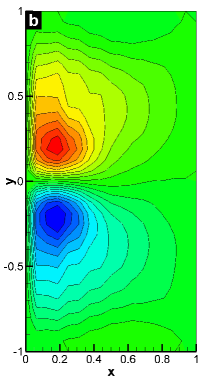
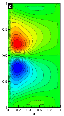
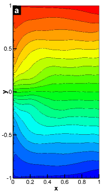
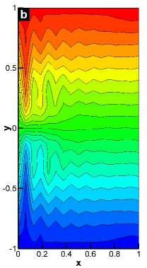
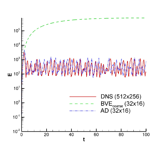
To summarize, the new AD model performs significantly better than the under-resolved BVE_coarse simulation in all tests. For the higher Reynolds number case the improvement is more dramatic. Indeed, the AD model correctly yields the four gyre pattern, just like the DNS computation, whereas the under-resolved BVE_coarse computation incorrectly predicts just two gyres. We also emphasize that the new AD model (resolution of $32\times 16$) is significantly more efficient than the DNS (resolution of $512\times 256$), yielding a speed-up factor of more than $1,000$.

Finally, we perform a sensitivity study with respect to the parameters used in the new AD model: $M$, the order of the high-order compact filter in Eq. (29); $N$, the order of the AD procedure in Eq. (16); and $\alpha$, the smoothing parameter of the second-order filter in Eq. (28). First, we investigate the sensitivity of the AD model with respect to $M$, the order of the high-order compact filter in Eq. (29). Since our tests show no significant differences among the different values of $M$, we are presenting below only the results obtained with the second-order filter in Eq. (28).

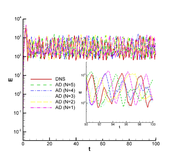
Next, we perform a sensitivity study with respect to $N$, the order of the AD procedure in Eq. (16). For a fixed smoothing parameter $\alpha=0.25$, the time-averaged streamfunction contour plots in Fig. (16) show a low sensitivity with respect to $N$. The time history of the total energy plotted in Fig. (17), however, displays a non-negligible sensitivity with respect to $N$. Indeed, higher values of $N$ yield more accurate results. Of course, the tradeoff is an increase in computational time due to the additional filtering operations needed for higher values of $N$: The CPU time is $170s$ for $N=5$, $145s$ for $N=3$, and $113s$ for $N=1$. Thus, the two numerical investigations in Fig. (16) and Fig. (17) seem to suggest that, in order to balance the numerical accuracy and the computational efficiency, a relative low value for $N$ might be desirable.

Figure 16: Experiment (ii):   Time-averaged streamfunction data for $Re=450$ and $Ro=0.0036$; Sensitivity with respect to the AD order $N$: (a) DNS results at $512\times 256$ resolution; (b) AD model results at a resolution of $32\times 16$ with $N=5$, (c) AD model results at a resolution of $32\times 16$ with $N=3$, (d) AD model results at a resolution of $32\times 16$ with $N=1$. Note the low sensitivity of the results with respect to $N$. Contour intervals are identical.

Figure 17: Experiment (ii):   Time history of the total energy for $Re=450$ and $Ro=0.0036$; Sensitivity with respect to the AD order $N$: DNS results at a resolution of $512\times 256$ and new AD model results at a resolution of $32\times 16$. Note the non-negligible sensitivity with respect to $N$. Embedded picture shows time series between t=90 and t=100.

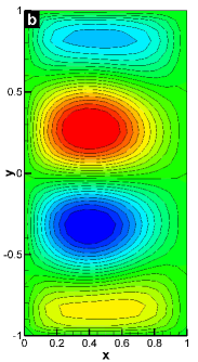
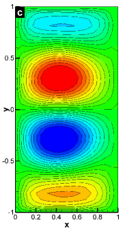
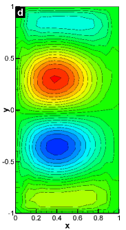
Finally, we investigate the sensitivity of the AD model with respect to $\alpha$, the smoothing parameter of the second-order filter in Eq. (28). For a fixed order of the AD procedure $N=5$, the time-averaged streamfunction contour plots in Fig. (18) show a low sensitivity with respect to $\alpha$. Our numerical experiments, however, suggest an optimal range of $0.1<\alpha<0.3$, since higher values of $\alpha$ do not eliminate numerical oscillations for coarse grids.

Figure 18: Experiment (ii):   Time-averaged streamfunction data for $Re=450$ and $Ro=0.0036$; Sensitivity with respect to the smoothing filtering parameter $\alpha$. (a) DNS results at a resolution of $512\times 256$; (b) AD model results at a resolution of $32\times 16$ with $\alpha=0.1$, (c) AD model results at a resolution of $32\times 16$ with $\alpha=0.25$, (d) AD model results at a resolution of $32\times 16$ with $\alpha=0.45$. Note the low sensitivity of the results with respect to $\alpha$. Contour intervals are identical.

6 Conclusions

This paper introduced a new approximate deconvolution (AD) model for the LES of two-dimensional turbulent geophysical flows. The AD model was tested in the numerical simulation of the wind-driven circulation in a shallow ocean basin, a standard prototype of more realistic ocean dynamics. The mathematical model employed was the barotropic vorticity equation (BVE) driven by a symmetric double-gyre wind forcing, which yielded a four-gyre circulation in the time mean. The AD model was tested on a mesh that was $16$ times coarser than that used by the direct numerical simulation (DNS) run. The AD model yielded numerical results that were in close agreement with those of the DNS. In particular, the four gyre structure of the time-averaged streamfunction contour plots was recovered by the AD model. Moreover, the CPU time of the AD model was 1,000 times lower than that of DNS. We emphasize that this combination of computational efficiency and numerical accuracy achieved by the new AD model was due to the specific subfilter-scale model utilized. Indeed, an under-resolved numerical simulation without any subfilter-scale model on the same coarse mesh as that employed by the AD model produced inaccurate results. We also performed a numerical investigation of the sensitivity of the new AD model with respect to the parameters used and we found that the model is robust. This first step in the numerical assessment of the new model shows that AD could represent a viable tool in the LES of more realistic turbulent geophysical flows.

References

- Adams and Stolz (2002) Adams, N., Stolz, S., 2002. A subgrid-scale deconvolution approach for shock capturing. J. Comput. Phys. 178 (2), 391–426.
- Arakawa (1966) Arakawa, A., 1966. Computational design for long-term numerical integration of the equations of fluid motion: Two-dimensional incompressible flow. Part I. J. Comput. Phys. 1 (1), 119–143.
- Awad et al. (2009) Awad, E., Toorman, E., Lacor, C., 2009. Large eddy simulations for quasi-2D turbulence in shallow flows: A comparison between different subgrid scale models. J. Marine Syst. 77 (4), 511–528.
- Batchelor (1969) Batchelor, G., 1969. Computation of the energy spectrum in homogeneous two-dimensional turbulence. Phys. Fluids 12, 233.
- Berselli et al. (2006) Berselli, L., Iliescu, T., Layton, W., 2006. Mathematics of large eddy simulation of turbulent flows. Springer Verlag.
- Bryan (1963) Bryan, K., 1963. A numerical investigation of a nonlinear model of a wind-driven ocean. J. Atmos. Sci. 20, 594–606.
- Chen et al. (2010) Chen, Q., Gunzburger, M., Ringler, T., 2010. A scale-invariant formulation of the anticipated potential vorticity method. Arxiv preprint arXiv:1010.2723.
- Chen et al. (2003) Chen, S., Ecke, R. E., Eyink, G. L., Wang, X., Xiao, Z., 2003. Physical mechanism of the two-dimensional enstrophy cascade. Phys. Rev. Lett. 91 (21), 214501.
- Cummins (1992) Cummins, P., 1992. Inertial gyres in decaying and forced geostrophic turbulence. J. Mar. Res. 50 (4), 545–566.
- Cushman-Roisin (1994) Cushman-Roisin, B., 1994. Introduction to geophysical fluid dynamics. Prentice Hall.
- Danilov and Gurarie (2000) Danilov, S., Gurarie, D., 2000. Quasi-two-dimensional turbulence. Phys. Usp. 43, 863.
- Dunca and Epshteyn (2006) Dunca, A., Epshteyn, Y., 2006. On the Stolz–Adams deconvolution model for the large-eddy simulation of turbulent flows. SIAM J. Math. Anal. 37, 1890.
- Fox-Kemper (2005) Fox-Kemper, B., 2005. Reevaluating the roles of eddies in multiple barotropic wind-driven gyres. J. Phys. Oceanogr. 35 (7), 1263–1278.
- Fox-Kemper and Menemenlis (2008) Fox-Kemper, B., Menemenlis, D., 2008. Can large eddy simulation techniques improve mesoscale rich ocean models? in Ocean Modeling in an Eddying Regime, Geophys. Monogr. Ser. 177, edited by M. Hecht and H. Hasumi, 319–338.
- Germano (2009) Germano, M., 2009. A new deconvolution method for large eddy simulation. Phys. Fluids 21, 045107.
- Gottlieb and Shu (1998) Gottlieb, S., Shu, C., 1998. Total variation diminishing Runge-Kutta schemes. Math. Comput. 67 (221), 73–85.
- Greatbatch and Nadiga (2000) Greatbatch, R., Nadiga, B., 2000. Four-gyre circulation in a barotropic model with double-gyre wind forcing. J. Phys. Oceanogr. 30 (6), 1461–1471.
- Griffa and Salmon (1989) Griffa, A., Salmon, R., 1989. Wind-driven ocean circulation and equilibrium statistical mechanics. J. Mar. Res. 47 (3), 457–492.
- Holland and Rhines (1980) Holland, W., Rhines, P., 1980. An example of eddy-induced ocean circulation. J. Phys. Oceanogr. 10 (7), 1010–1031.
- Holm and Nadiga (2003) Holm, D., Nadiga, B., 2003. Modeling mesoscale turbulence in the barotropic double-gyre circulation. J. Phys. Oceanogr. 33 (11), 2355–2365.
- Holton (2004) Holton, J., 2004. An introduction to dynamic meteorology. Academic Press.
- Kraichnan (1967) Kraichnan, R., 1967. Inertial ranges in two-dimensional turbulence. Phys. Fluids 10, 1417.
- Leith (1971) Leith, C., 1971. Atmospheric predictability and two-dimensional turbulence. J. Atmos. Sci. 28, 145–161.
- Lesieur (2008) Lesieur, M., 2008. Turbulence in fluids. Springer Verlag.
- Majda (2003) Majda, A., 2003. Introduction to PDEs and waves for the atmosphere and ocean. American Mathematical Society.
- Majda and Wang (2006) Majda, A., Wang, X., 2006. Non-linear dynamics and statistical theories for basic geophysical flows. Cambridge University Press.
- Marshall and Pillar (2011) Marshall, D., Pillar, H., 2011. Momentum balance of the wind-driven and meridional overturning circulation. J. Phys. Oceanogr. 41 (5), 960–978.
- McWilliams (1989) McWilliams, J., 1989. Statistical properties of decaying geostrophic turbulence. J. Fluid Mech. 198, 199–230.
- McWilliams (2006) McWilliams, J., 2006. Fundamentals of geophysical fluid dynamics. Cambridge University Press.
- Meneveau and Katz (2000) Meneveau, C., Katz, J., 2000. Scale-invariance and turbulence models for large-eddy simulation. Annu. Rev. Fluid Mech. 32 (1), 1–32.
- Moin (2001) Moin, P., 2001. Fundamentals of engineering numerical analysis. Cambridge University Press.
- Munk (1950) Munk, W., 1950. On the wind-driven ocean circulation. J. Meteor. 7 (2), 80–93.
- Munk and Wunsch (1982) Munk, W., Wunsch, C., 1982. Observing the ocean in the 1990s. Phil. Trans. R. Soc. Lond. A 307 (1499), 439–464.
- Nadiga and Margolin (2001) Nadiga, B., Margolin, L., 2001. Dispersive-dissipative eddy parameterization in a barotropic model. J. Phys. Oceanogr. 31 (8), 2525–2531.
- Özgökmen and Chassignet (1998) Özgökmen, T., Chassignet, E., 1998. Emergence of inertial gyres in a two-layer quasigeostrophic ocean model. J. Phys. Oceanogr. 28 (3), 461–484.
- Özgökmen et al. (2009) Özgökmen, T., Iliescu, T., Fischer, P., 2009. Large eddy simulation of stratified mixing in a three-dimensional lock-exchange system. Ocean Modell. 26 (3-4), 134–155.
- Sagaut (2006) Sagaut, P., 2006. Large eddy simulation for incompressible flows: An introduction. Springer Verlag.
- Salmon (1998) Salmon, R., 1998. Lectures on geophysical fluid dynamics. Oxford University Press.
- Smith et al. (2002) Smith, K., Boccaletti, G., Henning, C., Marinov, I., Tam, C., Held, I., Vallis, G., 2002. Turbulent diffusion in the geostrophic inverse cascade. J. Fluid Mech. 469, 13–48.
- Stanculescu (2008) Stanculescu, I., 2008. Existence theory of abstract approximate deconvolution models of turbulence. Ann. Univ. Ferrara 54 (1), 145–168.
- Stolz and Adams (1999) Stolz, S., Adams, N., 1999. An approximate deconvolution procedure for large-eddy simulation. Phys. Fluids 11, 1699.
- Stolz et al. (2001a) Stolz, S., Adams, N., Kleiser, L., 2001a. An approximate deconvolution model for large-eddy simulation with application to incompressible wall-bounded flows. Phys. Fluids 13, 997.
- Stolz et al. (2001b) Stolz, S., Adams, N., Kleiser, L., 2001b. The approximate deconvolution model for large-eddy simulations of compressible flows and its application to shock-turbulent-boundary-layer interaction. Phys. Fluids 13, 2985.
- Stolz et al. (2004) Stolz, S., Adams, N., Kleiser, L., 2004. The approximate deconvolution model for compressible flows: Isotropic turbulence and shock-boundary-layer interaction. in Advances in LES of Complex Flows, Fluid Mech. Appl. 65, edited by R. Friedrich and W. Rodi, 33–47.
- Tabeling (2002) Tabeling, P., 2002. Two-dimensional turbulence: a physicist approach. Phys. Rep. 362 (1), 1–62.
- Vallis (2006) Vallis, G., 2006. Atmospheric and oceanic fluid dynamics: fundamentals and large-scale circulation. Cambridge University Press.
- Visbal and Gaitonde (2002) Visbal, M., Gaitonde, D., 2002. On the use of higher-order finite-difference schemes on curvilinear and deforming meshes. J. Comput. Phys. 181 (1), 155–185.