On collisional capture rates of irregular satellites around the gas-giant planets and the minimum mass of the solar nebula

Abstract

We investigated the probability that an inelastic collision of planetesimals within the Hill sphere of the Jovian planets could explain the presence and orbits of observed irregular satellites. Capture of satellites via this mechanism is highly dependent on not only the mass of the protoplanetary disk, but also the shape of the planetesimal size distribution. We performed 2000 simulations for integrated time intervals $\sim 2$ Myr and found that, given the currently accepted value for the minimum mass solar nebula and planetesimal number density based upon the Nesvorný et al. (2003) and Charnoz & Morbidelli (2003) size distribution $dN\sim D^{-3.5}dD$, the collision rates for the different Jovian planets range between $\sim 0.6$ and $\lower 2.0pt\hbox{$\,\buildrel\scriptstyle>\over{\scriptstyle\sim}\,$}170\,{\rm\,Myr}^{-1}$ for objects with radii, $1\,{\rm\,km}\leq r\leq 10\,{\rm\,km}$. Additionally, we found that the probability that these collisions remove enough orbital energy to yield a bound orbit was $\lower 2.0pt\hbox{$\,\buildrel\scriptstyle<\over{\scriptstyle\sim}\,$}10^{-5}$ and had very little dependence on the relative size of the planetesimals. Of these collisions, the collision energy between two objects was $\lower 2.0pt\hbox{$\,\buildrel\scriptstyle>\over{\scriptstyle\sim}\,$}10^{3}$ times the gravitational binding energy for objects with radii $\sim 100$ km. We find that, capturing irregular satellites via collisions between unbound objects can only account for $\sim 0.1\%$ of the observed population, hence can this not be the sole method of producing irregular satellites.

1 Introduction

The irregular satellites of the Jovian planets have been the subject of much debate since their discovery in the early 1900’s. Since then there have been approximately 60 found around Jupiter, about 60 around Saturn, 20 around Uranus and 10 around Neptune (Gladman et al., 2001; Holman et al., 2004; Sheppard et al., 2006). Chamberlin & Yeomans (2010) present a current and detailed compilation of the irregular satellites (e.g. size, orbital characteristics, etc.) for the gas giant planets as well as a list of references containing these data.

Although a clear definition of an irregular satellite remains to be determined, we use the same definition as Nesvorný et al. (2003), moons that are far enough from their parent planet that the precession of their orbital plane is primarily controlled by the Sun. As stated in Nesvorný et al. (2003), this definition of an irregular satellite excludes Neptune’s moon Triton. The origin of these irregular satellites has yet to be clearly understood and can give an insight to the formation of our Solar system. Traditional theories of planet formation and evolution fail to produce the observed large orbital inclination observed for many of these satellites, some of which even follow retrograde orbits with respect to the orbital plane of the planets. Jewitt & Sheppard (2005) review the possible modes that possible modes of capturing irregular satellites by the giant planets are;

• Gas Drag: Similar to the Sun and Solar nebula, the gas giants are believed to be the result of the gravitational collapse of a planetary gas nebula. Therefore, it would be possible for irregular satellites to have enough energy dissipated by the planetary nebula via gas drag to remain gravitationally bound to the planet. Pollack et al. (1979) model these phenomena as a possible explanation for the capture and fragmentation of Jupiter’s prograde and retrograde irregular satellites, but don’t provide a clear explanation for the irregular satellites orbiting Uranus and Neptune. Furthermore, with out the dissipation of planetary nebula, once captured, the captured object would spiral into the planet $\sim 10$ yrs (Nesvorný et al., 2003).

• Pull Down: Pull down is the sudden mass-growth of the parent planet thereby capturing the satellite (Heppenheimer & Porco, 1977). This mode of capture occurs when an object enters the Hill sphere (region around a planet with radius, $R_{H}=a(m_{p}/\rm\,M_{\odot})^{1/3}$, where the Sun’s gravity is negligible compared the planet’s) through a Lagrange point and while at this semi-stable orbital point ($\sim 100{\rm\,yrs}$), the mass of the parent planet increases enough for the object to become gravitationally bound to the planet.

• Collisions: Gravitational three body interactions (both colliding and non-colliding) occurring within the Hill sphere of the planet could lead to the capture of one of the objects as well as fragments resulting from high energy collisions (Colombo & Franklin, 1971; Weidenschilling, 2002). Nesvorný et al. (2003) calculate the collision rate between the existing irregular satellites of Jupiter to be $\lower 2.0pt\hbox{$\,\buildrel\scriptstyle<\over{\scriptstyle\sim}\,$}1$ every 4.5 Gyr, implying that their formation hardens back to a time when the Solar system was much denser.

The purpose of this paper is to expand upon the last scenario, which has achieved some popularity in recent years. Nesvorný et al. (2004) that showed that the spectral characteristics of the irregular satellite groups around Jupiter and the other planets were surprisingly similar. This has been taken to suggest that they are all drawn from the same underlying progenitor population, and captured during the early dynamical evolution of the solar system. The most detailed scenario for such an evolution is the so-called Nice model for the solar system origin (Nesvorný et al., 2007; Bottke et al., 2010a). The initial conditions in this model are chosen to meet specific benchmarks of a larger scenario involving the explanation of various dynamical structures in the Solar system, and do seem to provide a path to capturing irregular satellites around some of the giant planets. Nevertheless, it is also useful to isolate the conditions necessary for a specific observable. Thus, in this paper we wish to evaluate the requirements of a simpler model, in which we determine the conditions that allow the irregular satellite populations to result from collisional interactions within the tidal field of a giant planet. This will also allow us to estimate the size of nebula that would match conditions necessary to the in situ formation of Uranus & Neptune proposed by Goldreich et al. (2004b). If irregular satellites could be the remnants of collisions that were captured by the planet as a result of said collision, collision rates and probabilities of remnants being captured by the planets could be used to set limits on the minimum mass Solar nebula (MMSN) as well as sizes and number densities of planetesimal seeds that eventually formed the inner planets, asteroid belt, Edgeworth-Kuiper belt objects and the Oort cloud.

The following section, § 2, briefly describes the epoch in the formation of the Solar system when the irregular satellites were most likely to have been captured. § 3 discusses why it is important for us to understand how these satellites were captured by their host planets. The presentation of how the data were generated, the motivation behind it and justification for it are contained in § 4.2, which is followed by a detailed description of how various probabilities were determined leading up to the calculation of the probability that a mass remains bound to a planet, § 5.1. The paper concludes with the results of these analyses, § 6, conclusions that can be drawn from these results, § 7, and suggested future work, § 8.

2 The Early Solar System: Seeds for Irregular Satellites

Goldreich et al. (2004b) and references therein give a detailed description of the early stages of planetary formation of our Solar system. The era most important to this investigation is that of oligarchy since this represents the time just prior to the formation of the inner terrestrial planets. At this point, the cores and the gas envelopes of the gas giant planets have already formed. Oligarchy is the point in the evolution of the Solar system where the formation of planets transferred from “runaway” growth to “ordered” growth (Kokubo & Ida, 1998). During this epoch, the planets in the outer Solar system had essentially finished forming, while the terrestrial planets were still acreting material. N-Body simulations presented in Goldreich et al. (2004a) and references therein show that for this to occur, the Solar nebula must be approximately equal in mass to the minimum mass in the inner Solar system and about six times the minimum mass of the Solar nebula in the outer solar system. This distribution of material is required to ensure the formation of Uranus and Neptune in their current location within the age of our Solar system (the actual surface densities used were $\sigma=7$g cm^-2 at 1 AU and $\sigma=1.5$ g cm ^-2 at 25 AU) (Goldreich et al., 2004b).

The epoch directly following oligarchy and thought to be the longest period in the evolution of our Solar system is “clean-up”. At the beginning of this phase of the evolution of our Solar system Jupiter and Saturn are likely to have been completely formed, Uranus and Neptune almost completely so. It is likely that $\lower 2.0pt\hbox{$\,\buildrel\scriptstyle>\over{\scriptstyle\sim}\,$}1000\;{\rm M}_{\earth}$ of small bodies were distributed amongst annulii with gravitational unstable orbits, to account for the expected distribution of $\sim 100\;{\rm M}_{\earth}$ of small bodies ejected by Uranus and Neptune and a current estimate of $1-10\;{\rm M}_{\earth}$ for the mass of the Oort cloud (Goldreich et al., 2004b).

3 Irregular Satellites: A Window to the Past

As stated in the first § 1, the irregular moons of the giant planets, like Edgeworth-Kuiper belt objects, are thought to be remnants of the early Solar system. With this in mind, an accurate description of their “capture” by their host planet and possibly the evolution of their bound orbits will provide insight to conditions in early Solar system.

As stated in § 1, it is difficult to produce a model where the irregular satellites form from the same circumplanetary disk from which the regular satellites formed, implying that the irregular satellites were captured by the planet through some other means. For these satellites to be captured through via collisions, the objects collide within the Hill sphere of the planet and this collision must dissipate enough energy to result in at least one of objects remaining gravitationally bound to the host planet. Therefore, we need to determine the probability that a planetesimal is located around the planet, then a distribution of where around the planet this object is most likely to be encountered by a second object. The probability of two objects colliding can be calculated from the product of these two distributions and a ratio of cross sectional areas (§ 6). Finally, a collision rate can be calculated by approximating the number of planetesimal present near the planets from accepted values of the minimum mass Solar nebula and assuming the density of these objects is comparable to that of the Earth.

4 Integration and Analysis

Expanding on the principle that these “small bodies” only weakly gravitationally interact with each other we chose to perform multiple simulations consisting of the Jovian planets, the Sun and only one small body, which is equivalent to a N-body integration containing $\lower 2.0pt\hbox{$\,\buildrel\scriptstyle>\over{\scriptstyle\sim}\,$}2000$ objects. Ideally we would have populated the orbital annuli gravitationally stirred by the planets with an oligarch number density equivalent to $\lower 2.0pt\hbox{$\,\buildrel\scriptstyle>\over{\scriptstyle\sim}\,$}100{\rm M}_{\oplus}$, but these numbers were computationally prohibitive. To avoid this complication, we assumed that oligarch-oligarch interactions can be ignored for N-body simulations run at the Solar system level due to their small relative mass. This allowed us to performed a large number of integrations containing only one “small body” following which we based the remaining analysis on probabilities. At the time of analysis, this methodology was preferred over a smaller number of simulations with a large number of bodies because parallel processing code to perform these operations was still being developed.

4.1 N-Body Integration

N-body integrations were perform using a Burlisch-Stoer integration routine embedded in the Mercury6 program written by Chambers (1999). The simulation integrates the orbital motions of the Jovian planets and one test mass for up to $8\times 10^{6}$ yrs or until the test mass either collides with a “big body” (planet or the Sun) or is ejected from the Solar system ($\lower 2.0pt\hbox{$\,\buildrel\scriptstyle>\over{\scriptstyle\sim}\,$}100{\rm\,AU}$ from the Sun). The accuracy used to define the time step for the integration was defined to be $\epsilon=10^{-15}$ to ensure accurate results calculated on a reasonable time frame. Using this parameter, integration time steps are determined by Press et al. (1997),

$$H_{k}=H\left(\frac{\epsilon}{\epsilon_{k+1,k}}\right)^{1/(2k+1)}$$ (1)

where, $H$ is the user defined time step and $\epsilon_{k+1,k}$ is the percent difference between the $k$ time steps and $k+1$ time steps to span $H$. Mercury6 provides tools to monitor “close encounters” between the different objects given the two objects pass within a user defined distance (Chambers, 1999). The distance defined to be the minimal distance defining a “close encounter” was a half of a Hill radius,

$$0.5R_{H}=0.5\,a_{p}\left(\frac{M_{p}}{\rm\,M_{\odot}}\right)^{1/3}$$ (2)

Originally the Mercury6 algorithm returned the orbital parameters of the two objects that pass within the predefined distance, but we altered the code to return the position and velocity vectors of the small mass measured with respect to the planet, which were then stored for further analysis.

4.1.1 Initial Conditions

The orbital parameters used to define the initial orbits of the small bodies were all generated randomly with the exception of the eccentricity, which is initially chosen to be equal to zero because this is the parameter most sensitive to gravitational perturbation and had quickly become randomized during the simulation. In order to reduce the number of simulations that led to stable orbits that do not interact with any of the planets, the initial semi-major axis is generated by randomly choosing an orbital annulus that Ito (2002) have shown to produce unstable orbits in our Solar system and then equated to a random number that would lie within one of these rings. Other than the argument of perigee and the ascending node, which were chosen to be randomly generated numbers between 0 and $2\pi$, the angle of inclination was a randomly generated number between $\pm 0.01^{\circ}$. Orbital inclinations within this range are well within the angular thickness of the Solar nebula after it began to “flatten”, allow for orbits crossing the planets beyond their orbital planes, and are low enough to ensure that the small bodies had orbits crossing the planets. Although planetesimals could have initially had large orbital inclinations, objects with inclinations much larger than those chosen were less likely to enter a planet’s Hill sphere. Furthermore, this range of inclinations still allows objects to pass through a planet’s Hill sphere with essentially a uniform distribution as expected. We found (as expected) that the probability of locating an object in a “bin” or region around the planet, $\mathcal{P}_{bin}=\langle t_{bin}/t_{tof}\rangle$ has essentially no radial nor angular dependence.

4.2 Analysis of N-Body Integration

Following the numerical integration performed with Mercury6, a more detailed analysis of the encounters between the small body and planet(s) was performed. Mercury6 generated vast quantities of data consisting of the initial positions and velocities of the small body with respect to the planet whenever the small body passed within $0.75\,R_{H}$ of the planet. These data were then used to calculate the fractional time spent within any given volume element, $dV$,

$$dV=\prod_{i=1}^{3}\Delta x_{i}$$

around the planet. Due to computational limitations (i.e. RAM as well as CPU capacity), $dV$ was restricted to be equal to $\sim 10^{-7}R_{H}^{3}$ corresponding to a Cartesian grid from $-0.75\,R_{H}$ to $0.75\,R_{H}$ in each direction consisting of 100 bins or divisions setting $\Delta x=0.15\,R_{H}$.

The time, $dt$, spent in each bin for a given pass through the Hill sphere is

$$dt=\frac{ds}{v}$$ (3)

where $ds$ is the path of the small body through the volume element and both $d\mathbf{s}$ and $\mathbf{v}$ point in the same direction. $dt_{i}$ is approximated by assuming that the small body is moving along a straight line through the bin and would therefore be equal to

$$dt_{i}={\rm\,min}\left(\frac{\Delta x_{i}}{v_{i}}\right)$$ (4)

where $\Delta x_{i}$ is the distance to the edge of the volume bin in the $i^{{\rm\,th}}$ direction where, $i=1,2,3$ represent the traditional Cartesian directions, $x$, $y$ and $z$ respectively.

In order to determine the probability of a small body being in the $j^{{\rm\,th}}$ bin, $dt$ is then scaled by the time-of-flight of the small body across the Hill sphere, or the amount of time required for the small body to pass through our region of interest around the planet ($\sim 0.75R_{H}$),

$$t_{tof}=\sqrt{\frac{a^{3}}{\mu}}\left(e\sinh F-F\right)$$ (5)

where $F$ is the hyperbolic eccentric anomaly,

$$\cosh F=\frac{e+\cos\varphi}{1+e\cos\varphi}$$

and $e$ is the eccentricity, $a$ is the semi-major axis and $\varphi$ is the angular measure from periapse. The ratio of $dt$ to $t_{tof}$ provides the fractional time spent per encounter in any given volume bin.

4.2.1 Regularly Spaced Propagation of Trajectory for to Determine Where Objects are Likely to be Found within the Hill Sphere for Unbound Trajectories

The trajectory of the small body through a planet’s Hill sphere was calculated from the angle measured from perigee, $\varphi$, and performing a coordinate transformation from the orbital coordinates, $x^{\prime}$, $y^{\prime}$, to a coordinate system fixed to the planet where the $x-y$ plane is at the planets equator and the $x$ axis is directed in the same direction as the $x$ axis use for the Solar system. Mathematically, the $x-y$ components of the position and velocity vectors in the orbital plane are;

$$x^{\prime} = r\cos\varphi$$ (6)

$$y^{\prime} = r\sin\varphi$$ (7)

$$v_{x} = -\frac{na}{\sqrt{1-e^{2}}}\sin\varphi$$ (8)

$$v_{y} = \frac{na}{\sqrt{1-e^{2}}}\left(e+\cos\varphi\right)$$ (9)

where

$$r=\frac{a\left(1+e^{2}\right)}{1+e\cos\varphi}$$ (10)

and $a$ is the semi-major axis, $e$ is the eccentricity of the small bodies trajectory past the planet calculated from the initial position and velocity of the small body as it enters the sphere of interest, and $\mu=n^{2}a^{3}$. This vector is then rotated to determine where in the planet’s fixed reference frame the object is located.

$$\mathbf{X}=\mathbf{\mathcal{R}}(\Omega)_{z^{p}}\mathbf{\mathcal{R}}(i)_{x^{\prime}}\mathbf{\mathcal{R}}_{z^{sb}}\mathbf{X}^{\prime}$$ (11)

where $\omega$ is the argument of perigee, $\Omega$ is the ascending node and $i$ is the angle of inclination and $\mathbf{\mathcal{R}}$ are the rotation matrices around the $z$ axis in the small body’s orbital plane, an intermediate $x$ axis and the $z$ axis in the planet’s orbital plane given by;

$$\mathbf{\mathcal{R}}(\Omega)_{z^{p}} = \left(\begin{array}[]{ccc}\cos\Omega&\sin\Omega&0\\ -\sin\Omega&\cos\Omega&0\\ 0&0&1\end{array}\right)$$ (15)

$$\mathbf{\mathcal{R}}(i)_{x^{\prime}} = \left(\begin{array}[]{ccc}1&0&0\\ 0&-\sin i&\cos i\\ 0&\cos i&\sin i\end{array}\right)$$ (19)

and

$$\mathbf{\mathcal{R}}(\omega)_{z^{sb}}=\left(\begin{array}[]{ccc}\cos\omega&\sin\omega&0\\ -\sin\omega&\cos\omega&0\\ 0&0&1\end{array}\right)$$

All of the positions and velocities calculated in the orbital frame are transformed using equation (11), which are then used to determine $dt$ and which bin it corresponds to. There were two reasons for simulating the orbit in this manner. The most important reason was that moving a small body along its trajectory in discrete angular steps that correspond to the angular width of the bins most distant from the planet ensures that the trajectories are sampled completely. Since most optimized integration routines will adjust the time step to ensure that there is a tolerable offset in a conserved quantity like the total energy or angular momentum, it is likely that some statistical bins located farthest from the planet would be “skipped” over. Therefore the angular step $\Delta\varphi=1.5\times 10^{-2}$ radians was used to correspond to the angular width of a bin at the farthest distance of interest, $\Delta x/R_{max}$, where $R_{max}=3/4\,R_{H}$. To a lesser extent, there is some reduced run-time because Mercury6 writes data to the hard disk at regular intervals, which would then need to be extracted to determine the trajectories.

5 Calculation of Probabilities

We calculated the probability of a physical collision between planetesimals occurring at a given region in space around the planet from three specific ratios; (1) the fraction of time spent in the area of interest around the planet, (2) the fraction of time spent per bin around the planet and (3) the fraction of cross sectional areas (i.e. a ratio of the small body cross section to the cross sectional area of the region of interest).

As stated in § 4.2.1, the fractional time spent in the $i^{th}$ volume bin is equal to $dt_{i}/t_{tof}$. The fraction of time spent around the planet is equal to $t_{{\rm\,planet}}/t_{int}$. For each integration performed, the time a small body “spends” around the planet was calculated by totaling the time of flight for each “close encounter” for that integration,

$$t_{{\rm\,planet}}=\sum_{j}\left(t_{tof}\right)_{i}$$ (20)

Mercury6 was configured to return the total integration time, $t_{int}$, for each run since the program would exit if the small body collided was ejected of if it collided with a large body (a planet or the Sun).

The probability that an object is in a given bin, $\mathcal{P}_{bin}$, provided the object is passing through a planet’s Hill sphere is,

$$\mathcal{P}_{bin}=\left(\frac{dt}{t_{tof}}\right)_{bin}\Big{\langle}\frac{t_{{\rm\,planet}}}{t_{int}}\Big{\rangle}.$$ (21)

Angular dependencies were neglected because $P_{bin}$ varied by less than 1 % over $4\pi$ sr. Although this conveys useful information, it is difficult to visualize. More information could be gathered from a temporal distribution along a trajectory to determine where in the Hill sphere these collisions could occur. Since, $dt_{i}/t_{tof}$ has little angular dependence, we assumed $dt_{i}/t_{tof}$ to be constant over all angles, hence an average $dt_{i}/t_{tof}$ over $4\pi$ sr would be comparable to averaging multiple temporal distributions to find $\langle dt/t_{tof}\rangle_{r}$.Therefore, the probability density of finding a small body in a given annulus at a given distance ($r+dr$) per cubic AU from the planet, within the planet’s Hill sphere is,

$$\mathcal{P}_{r}=\Big{\langle}\frac{dt}{t_{tof}}\Big{\rangle}_{r}\Big{\langle}\frac{t_{{\rm\,planet}}}{t_{int}}\Big{\rangle}$$ (22)

The probability that two objects occupy the same bin along a trajectory through a planet’s Hill sphere can be found by integrating the probability density $\mathcal{P}_{r}$ along an object’s trajectory. If these objects were large enough to occupy the entire volume of a “bin”, this would then be the probability of two objects colliding. Unfortunately this is not the case and this integration must therefore be re-scaled by the ratio of the two cross-sectional areas,

$$\frac{\tilde{\sigma}_{sb}}{\sigma_{bin}} = \frac{\pi r_{sb}^{2}}{\Delta x^{2}}$$ (23)

$$= \frac{80}{9}\frac{r^{2}_{sb}}{R^{2}_{H}}\pi\times 1000$$

If there were only two objects in a planet’s Hill sphere at any given time, then we would only need the ratio of $\tilde{\sigma}_{sb}$ to $\sigma_{bin}$. Since it is likely that there multiple small bodies in the Hill sphere, $\tilde{\sigma}_{sb}$ needs to be scaled by the number of small bodies present, $N\,\mathcal{P}_{{\rm\,planet}}$, where $N$ is the total number of small bodies on the annulus that interact with the planet and $\mathcal{P}_{{\rm\,planet}}=\langle t_{{\rm\,planet}}/t_{int}\rangle$, leading to a cross sectional ratio of

$$\frac{\sigma_{sb}}{\sigma_{bin}}=n(r_{sb};M_{\rm MMSN})\mathcal{P}_{{\rm\,planet}}\frac{80}{9}\frac{\pi r_{sb}^{2}}{R_{H}^{2}}\times 10^{3}.$$ (24)

where $n(r_{sb};M_{\rm MMSN})$ are the number of objects with radius $r_{sb}$ and properly scales the area occupied by the “small bodies”. The total area occupied by the planetesimals will be this ratio, integrated over all radii (or at least the radii of interest - 1 to 200 km). Lastly, all of these pieces need to be brought together to yield the probability that any two small bodies will collide within the Hill sphere of a planet.

$$\tilde{\mathcal{P}}_{col}(r) = \int\mathcal{P}^{2}_{r}dV\frac{\sigma_{sb}}{\sigma_{bin}}$$

$$= n(r;M_{\rm MMSN})\int\Big{\langle}\frac{dt}{t_{\rm tof}}\Big{\rangle}^{2}_{r}dV\Big{\langle}\frac{t_{{\rm planet}}}{t_{\rm int}}\Big{\rangle}^{2}\frac{\pi r_{sb}^{2}}{\Delta x^{2}}.$$

Assuming that the rocky material in the Solar nebula is uniformly distributed, the surface density of this material for the Solar nebula disk between Jupiter and Neptune is

$$\sigma_{SN}\sim\frac{100\rm\,M_{\oplus}}{\pi\left(30^{2}-5^{2}\right){\rm\,AU}^{2}}$$ (26)

The number density of small bodies orbiting the Sun was calculated based upon the size distribution of planetesimals presented in Nesvorný et al. (2003) and Charnoz & Morbidelli (2003). The number of small bodies as a function of the MMSN was assumed to be

$$n(r;M_{\rm MMSN})=\eta(M_{\rm MMSN})r^{-1.8}$$ (27)

where

$$\eta=\frac{M_{\rm MMSN}}{\rho_{\oplus}}\left[\int r^{-1.8}V(r)dr\right]^{-1},$$

$V(r)$ is the volume of the planetesimal and $\rho_{\oplus}$ is the density of the Earth. Lastly equation (5) must be integrated over all “small body” radii and the total probability that two planetesimals collide within a planet’s Hill sphere is

$$\mathcal{P}_{col} = \int\tilde{\mathcal{P}}_{col}(r)dr$$

$$= \frac{M_{\rm MMSN}}{\rho_{\oplus}}\left[\int\tilde{r}^{-1.8}V(\tilde{r})d\tilde{r}\right]^{-1}\int r^{-1.8}\frac{r^{2}}{\Delta x^{2}}dr$$

$$\times \int\Big{\langle}\frac{dt}{t_{\rm tof}}\Big{\rangle}^{2}\Big{\langle}\frac{t_{\rm planet}}{t_{\rm int}}\Big{\rangle}^{2}dV$$

where the integration over $dV$ is the volume of the Hill sphere and the integrations over both $r$ and $\tilde{r}$ are with respect to “small body” radii given by Nesvorný et al. (2003) and Charnoz & Morbidelli (2003) size distribution of $dN\propto D^{-3.5}dD$.

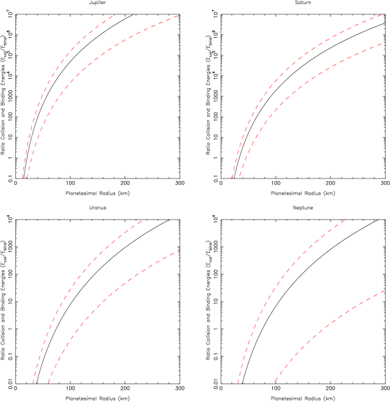
Figure 1: Ratio of collision energy $E_{{\rm col}}$ to gravitational binding energy $E_{{\rm bind}}$ as a function of the “small body” (planetesimal) radius. The (red) dashed lines represent one $\sigma$ error for the measured collision energies. The (red) dashed lines correspond to the measured uncertainty of $E_{{\rm col}}$

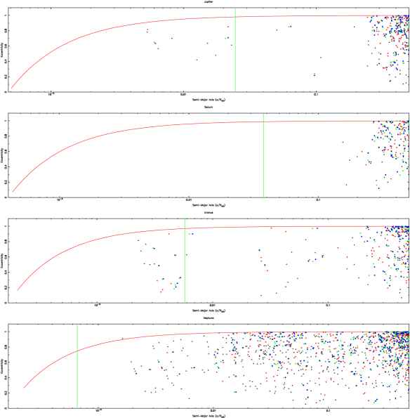
Figure 2: Eccentricity plotted as a function of Semi-Major axis for the conglomerate generated by the collision of two objects within Jupiter’s Hill sphere. The region above the (red) line correspond to the bound orbits that pass within Jupiter’s radius thereby resulting in a collision with the planet and the vertical (green) line the semi-major axis of the “regular” moon orbiting farthest from the planet. There are no restrictions placed on the collision energy for the points plotted above and the average value for $V_{col}^{2}$ is $\sim 4\times 10^{3}\mu_{sb}/r_{col}$, the binding energy per unit object of the small body where we assumed $r_{col}\sim 10{\rm\,km}$. The different points correspond to different object ratios between the colliding objects: (black) triangle are 1 to 1, (red) diamonds are 10 to 1, (green) pentagons are 100 to 1 and (blue) hexagons are 1000 to 1.

5.1 Probability of a Bound Orbit and the Resulting Orbital Parameters

The majority of collisions that occurred in a planet’s Hill sphere did not result in the object remaining gravitationally bound to that planet. The magnitude of the kinetic energy of a typical collision is extremely high (figure 1) and is large enough to completely destroy objects with radii $\lower 2.0pt\hbox{$\,\buildrel\scriptstyle<\over{\scriptstyle\sim}\,$}20{\rm\,km}$. Furthermore, even if the two objects were able to coalesce, the majority of collisions did not remove sufficient orbital energy from the combined object to result in a bound orbit.

However, to simplify matters, we can make some initial assumptions about the dynamics of a collision needed to be made in order to determine which collisions would result in a bound orbit or not and revisit these assumptions given the results. The first assumption was that the two objects would “stick” together, or

$$\big{|}\mathbf{v_{1}}-\mathbf{v_{2}}\big{|}<\sqrt{2G\rho r_{sb}^{2}}$$ (29)

where the objects have a density, $\rho_{sb}$, equal to the density of the Earth, $\rho_{\oplus}\approx 5{\rm g\,}{\rm cm}^{-3}$. We understand that this is not the case, but calculating the orbital characteristics of the resulting inelastic collision is simpler and can serve as a lower limit for the probability of objects being captured. Although technically not an assumption, the trajectories known to pass through a given volume bin ($d\lower 2.0pt\hbox{$\,\buildrel\scriptstyle<\over{\scriptstyle\sim}\,$}0.01{\rm\,AU}$, where $d$ is the distance between the two objects) were “forced” to collide by translating the small bodies to the average position vector with their given velocity. This translation results in a error of $\lower 2.0pt\hbox{$\,\buildrel\scriptstyle<\over{\scriptstyle\sim}\,$}1\%$, and the probability of a collision occurring was already determined in equation 5. Furthermore the ensemble required to produce even one collision is prohibitively large, “forcing” trajectories to “cross paths” is a reasonable approximation (assumption). Lastly, provided equation (29) is satisfied, a collision results in a bound orbit provided,

$$V_{cm}^{2}<2\frac{GM_{{\rm\,planet}}}{r_{col}}$$ (30)

where $\mathbf{V_{cm}}=(m_{1}\mathbf{v_{1}}+m_{2}\mathbf{v_{2}})/(m_{1}+m_{2})$ is the center of mass velocity, $\mathbf{r_{col}}=(\mathbf{r_{1}}+\mathbf{r_{2}})/2$ is the point where the collision is “forced” to occur and that the agglomerate doesn’t smash into the planet (i.e. $a(1-e)>r_{{\rm\,planet}}$).

Initial conditions for trajectories corresponding with all of the “close encounters” for each planet were stored so that we could use each unique initial condition to integrate trajectories and determine collision characteristics. Limiting ourselves to 500 unique initial conditions, we assign an initial condition to one object, then step through the remaining conditions counting the total number of “assumed” collisions ($d<\sqrt{2}\Delta x$), $N_{c}$, and the number that result in a bound orbit, $N_{b}$ (resulting object satisfying equation 30). This results in

$$\sum_{i=2}^{500}i\left(i-1\right)\sim 4\times 10^{7}$$

integrations. These integrations produced $\sim 10^{5}$ collisions of which $\lower 2.0pt\hbox{$\,\buildrel\scriptstyle<\over{\scriptstyle\sim}\,$}10$ resulted in a bound orbit (table LABEL:tab:ProbBound).

Figure (2) are plots of the eccentricity as a function of semi-major axis for an irregular satellite captured by the planets via an inelastic collision between two planetesimal. This plot shows that the eccentricities of orbits arising from these collisions are essentially random, although slightly skewed with a mean of $\sim 0.7$. The region above the line corresponds to orbits with periapse less than or equal to the radius of the planet (in this case Jupiter). These orbits would result in a collision with the planet. Additionally, figure (4) shows the distribution of inclinations from the resulting bound orbits. These distributions are essentially random distributions with a couple of the planets having a slightly higher probability of orbits with marginally retrograde orbits with inclinations $\sim 120\deg$.

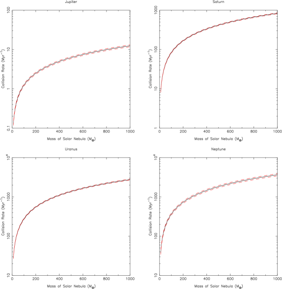
Figure 3: Collision rates for small body collisions occurring within the planet’s Hill sphere. The number of small bodies from calculated using equation (27) is used in conjunction with equation (5) to calculate collisions per Myr. The (red) dashed lines correspond with the propagated measurement uncertainty of $\langle dt/t_{tof}\rangle_{r}$ and $\langle t_{\rm planet}/t_{int}\rangle$

(a) Jupiter

(b) Saturn

(c) Uranus

(d) Neptune

Figure 4: Distribution of the angle of inclination for the bound orbits represented in figure 2. As stated in the assumptions, these inclinations are the result of a collision between to planetesimals within a Jovian planets’ Hill sphere where the two objects “stuck” together.

6 Results

We ran 2000 random simulations resulting in $\lower 2.0pt\hbox{$\,\buildrel\scriptstyle>\over{\scriptstyle\sim}\,$}2\times 10^{8}$ close encounters between a given planet and a test mass that revealed the mean fractional times, $\langle t_{{\rm\,planet}}/t_{int}\rangle$ spent around Jupiter, Saturn, Uranus and Neptune are $5.48\times 10^{-5}$, $5.32\times 10^{-5}$, $1.31\times 10^{-5}$ and $6.29\times 10^{-5}$ respectively (described in § 5). As stated in § 4.1, numerical integrations simulated periods of $\sim 8{\rm\,Myrs}$ unless the test mass was ejected or collided with either a planet or the Sun prior to the 1 Myr period being completed. Although we attempted to place the test masses on known unstable orbits around the Sun determined from Ito (2002), $\sim 40\%$ of the simulations ran the entire $8{\rm\,Myrs}$, $\sim 25\%$ ended $\lower 2.0pt\hbox{$\,\buildrel\scriptstyle<\over{\scriptstyle\sim}\,$}1{\rm\,Myr}$ and the remaining $35\%$ uniformly distributed between $1-5{\rm\,Myrs}$.

Table 1: Collision Rate of Irregular Satellites (Myr^-1)

Object Radius (km)	Jupiter	Saturn	Uranus	Neptune
$1\leq r\leq 10$	$0.601\pm 0.304$	$40.30\pm 1.25$	$133.1\pm 4.2$	$176.3\pm 11.0$
$10\leq r\leq 100$	$(1.90\pm 0.11)\times 10^{-3}$	$(1.28\pm 0.04)\times 10^{-1}$	$(4.21\pm 0.13)\times 10^{-1}$	$(5.57\pm 0.35)\times 10^{-1}$
$100\leq r\leq 1000$	$(6.01\pm 0.34)\times 10^{-7}$	$(4.03\pm 0.01)\times 10^{-3}$	$(1.33\pm 0.04)\times 10^{-3}$	$(1.76\pm 0.11)\times 10^{-3}$

Using the formulae presented in § 5, we found that the fractional time that a test mass spends around any given planet was $\sim 10^{-5}$, therefore if an object remained gravitationally bound to the Sun on an unstable orbit for $1{\rm\,Myr}$ it would be likely to spend $\sim 50{\rm\,yr}$ within the Hill sphere of any one of Jovian planets. Assuming that the MMSN is $\sim 100\,\rm\,M_{\oplus}$, collision rates for varying object sizes are presented in table (1). For object radii between 1 and 10 km, collision rates are $0.601\pm 0.304\,{\rm\,Myr}^{-1}$for Jupiter, $40.3\pm 1.25\,{\rm\,Myr}^{-1}$for Saturn $133.1\pm 4.2\,{\rm\,Myr}^{-1}$ for Uranus and $176.3\pm 11.0\,{\rm\,Myr}^{-1}$ (figure 3) for Neptune. Although these collision rates may appear to be large and imply that there should be a significantly larger population of irregular satellites, when combined with the probability that a collision between two planetesimal results in a bound orbit, capture rates for objects with radii between 1 and 10 km are (table 2) $(2.00\pm 0.22)\times 10^{-5}\,{\rm\,Myr}^{-1}$, $(6.74\pm 0.64)\times 10^{-4}\,{\rm\,Myr}^{-1}$, $(4.19\pm 0.46)\times 10^{-3}\,{\rm\,Myr}^{-1}$, $(6.40\pm 0.52)\times 10^{-3}\,{\rm\,Myr}^{-1}$, for Jupiter, Saturn, Uranus and Neptune respectively, for a MMSN of $\sim 100\rm\,M_{\oplus}$. Given energies plotted in figure 1, it is possible that a collision between an object with radius $\sim 10{\rm\,km}$ collided with one with a radius of $\sim 100{\rm\,km}$, which would have resulted in the larger of the two being broken apart. Another point of interest is that Jupiter has a “capture” rate significantly lower than the other planets. This is most likely due to the fact that as these objects move closer to the Sun, their speed increases, thereby requiring more energy to be removed when the two planetesimals collide in order to capture the satellite.

Table 2: Capture Rate of Irregular Satellites (Myr^-1)

Object Radius (km)	Jupiter	Saturn	Uranus	Neptune
$1\leq r\leq 10$	$(2.00\pm 0.10)\times 10^{-5}$	$(6.74\pm 0.64)\times 10^{-4}$	$(6.74\pm 0.64)\times 10^{-4}$	$(4.19\pm 0.46)\times 10^{-3}$
$10\leq r\leq 100$	$(6.32\pm 0.69)\times 10^{-8}$	$(2.13\pm 0.20)\times 10^{-6}$	$(1.33\pm 0.15)\times 10^{-5}$	$(2.02\pm 0.17)\times 10^{-5}$
$100\leq r\leq 1000$	$(2.00\pm 0.22)\times 10^{-10}$	$(6.74\pm 0.64)\times 10^{-9}$	$(4.19\pm 0.46)\times 10^{-8}$	$(6.40\pm 0.52)\times 10^{-8}$

7 Conclusions

The Jovian planets are known to have between $\sim 20$ and $\sim 60$ irregular satellites orbiting them depending on the planet (Jupiter $\lower 2.0pt\hbox{$\,\buildrel\scriptstyle>\over{\scriptstyle\sim}\,$}60$, Neptune $\sim 10$). Assuming that these satellites were all captured over a period of 1-2 Myrs, the “capture rates” for the planets would be $\sim 0.001{\rm\,Myr}^{-1}$. In § 6 we present the probability that a collision resulted in a bound orbit $P_{\rm bound}\sim 10^{-5}$ per Myr for a total MMSN containing about $100\,\rm\,M_{\oplus}$ and object radii $1{\rm\,km}\leq r\leq{\rm\,km}$. The collision energy scaled by the binding energy of an object with a 100 km radius (figure 1) shows that collisions between the different objects would have to have a mass ratio $\lower 2.0pt\hbox{$\,\buildrel\scriptstyle<\over{\scriptstyle\sim}\,$}0.1$ to ensure that both weren’t completely destroyed and a ratio of $\sim 1$ to be broken apart and not reduced to rubble. Using a MMSN based upon asteroid measurements presented by Morbidelli et al. (2009), which is $\eta_{MMSN}\sim 10^{6}{\rm\,AU}^{-2}$ and size distribution given in (Nesvorný et al., 2003; Charnoz & Morbidelli, 2003), $dN\propto D^{-3.5}dD$, the rate the Jovian planets could expect to capture irregular satellites through collisions is $\sim 10^{-3}{\rm\,Myr}^{-1}$ (figure 3). This would be consistent with the Goldreich et al. (2004b) oligarchy models with the exception that objects primarily consist of $\lower 2.0pt\hbox{$\,\buildrel\scriptstyle>\over{\scriptstyle\sim}\,$}10-100$ km sized objects, not $\sim 1$ km and requiring a slightly larger MMSN in order to populate the Edgeworth-Kuiper belt, asteroid belt and Oort cloud. Since the probability is highly dependent upon the size distribution of planetesimals as well as the mass of the protoplanetary disk, we also investigated size distributions of $dN\propto D^{1.8}dD$ (Bottke et al., 2010b), $dN\propto D^{-2.2}dD$ and $dN\propto D^{-2.8}dD$ (Terai & Itoh, 2010) all producing similar results for object radii $10{\rm\,km}\leq r\leq 100{\rm\,km}$ (e.g. same order of magnitude). However for $1{\rm\,km}\leq r\leq 10{\rm\,km}$, collision rates for a size distribution $dN\propto D^{-1.8}dD$ is approximately half that for $dN\propto D^{-3.5}dD$ and for the radii $100{\rm\,km}\leq r\leq 1000{\rm\,km}$ its approximately doubled. As the magnitude of the power law increases, naturally the probability of collisions increases for smaller objects because there are a larger number of them. Furthermore, allowing planets to migrate as in the Nice model or simulated by Lykawka et al. (2009), each planet would sweep through a larger effective area, thereby marginally increasing the probability of a collision between objects.

The results presented above are subject to some caveats.

• The two objects colliding, “stick” together and form a single object as a result of the collision, which can not be the case because the collision energies are $\lower 2.0pt\hbox{$\,\buildrel\scriptstyle>\over{\scriptstyle\sim}\,$}10$ times the gravitational binding energy. This assumption can result in an underestimation in the orbital energy removed from the collision and lead to an underestimation of the number of bound satellites.

• The objects are assumed to never achieve a “quasi-bound” orbit, which is known to occur where objects can remain “bound” to the planet for more than 100 years. Although these objects are rare, the amount of time spent within the Hill sphere is $\lower 2.0pt\hbox{$\,\buildrel\scriptstyle>\over{\scriptstyle\sim}\,$}10^{4}$ times those scattering off of the planet. Furthermore since these objects are already on a “quasi-bound” orbit around the planet, less energy needs to be removed from the collision. Each of the impacts from this assumption, like the first, would lead to an underestimate of the number of bound satellites. Horner & Wyn Evans (2006) have shown that the Centaurs can be capture like Trojan satellites and even irregular satellites are able to be temporarily captured by Jupiter for $\lower 2.0pt\hbox{$\,\buildrel\scriptstyle>\over{\scriptstyle\sim}\,$}10^{4}$ years. Also, in recent years a number of comets, Gehrels, Shoemaker-Levy 9 and Oterma Ohtsuka et al. (2008) and references therein. Furthermore, Horner & Lykawka (2010) have shown such captures to be quite frequent. Such events could significantly boost our capture rates.

• All of the planets formed at there present location. It has already been accepted that, at least, Neptune has migrated outward since its formation (Malhotra, 1993). As planet migrated away from the Sun, there Hill sphere increases, which would mean that for planets moving outward (Neptune and Uranus), their Hill spheres would have been over estimated, hence the probability of capture as well. We believe that this over estimation is compensated by the fact that as the planet(s) migrated the annulus swept out by their orbit(s) grows giving them “access” to a larger number of objects. However, for planets that migrated inward, their Hill spheres were underestimated, this coupled with the “growth” of their orbital annulii would lead to an underestimation of the number of bound satellites.

• The density of objects colliding is $\sim\rho_{\oplus}$, where in actuality the density is less than the density of the Earth because the Earth and Mercury are the objects with the greatest known density. This will lead to an underestimate in the number of objects (planetesimals), hence produce an artificially low collision rate.

We found that collisions between objects with a mass ratio as large as 1000 to 1 only marginally reduce the capture rate (probability of bound orbits listed in table LABEL:tab:ProbBound). It is possible for a large mass to collide with a smaller mass and, though the smaller of the two would be destroyed because the collision is large enough to reduce the small mass to rubble, the larger mass would fare much better and would most likely simply be broken apart, resulting in some of the debris from the collision remaining bound to the planet. Furthermore, since $\sim 1000$ 1 km radius objects are contained in a mass with a 100 km radius, it is possible that only a small fraction of the remnants from the collision could remain bound to the planet were the remainder did not have enough energy dissipated by the collision. A detailed analysis of the collisions of these objects and simulations of the distribution would need to be done to determine what fraction of these remnants would remain bound to the planets.

We found that the average semi-major axes for bound orbits are essentially randomly distributed between 0.3 and 2 Hill radii, which is consistent with observation with the exception that many of the objects captured in the simulation had highly eccentric orbits and many with a semi-major axis $\lower 2.0pt\hbox{$\,\buildrel\scriptstyle>\over{\scriptstyle\sim}\,$}5$ Hill radii, which is not what has been observed. This is most likely because these objects were probably stripped from the planet by the Sun’s gravity or interacted with the regular satellites to produce more circular orbits, closer to the planet. The act of satellites being stripped from the planets’ orbit is yet another factor not accounted for in the analysis above. Since nearly half the capture objects have orbits that are on the outer cusp of the Hill sphere, either their orbits would have to decay, or they would be stripped from the planet.

Although it is unlikely that all of the irregular satellites were captured via collisions with the host planet’s Hill sphere, we have shown that there is a finite probability that irregular satellites can be capture through collisions, which would serve as a lower limit based on the assumptions that have been made. Additionally, the large collision energies that we measured would be consistent with the observations of Nesvorný et al. (2004) who state that some of Jupiter’s irregular satellites can be clustered into specific groups with similar orbital elements and spectral characteristics.

8 Further Work

There are several issues that need to be addressed in future work, which can be subdivided into two different sections. One section incorporates the assumptions made in the simulations performed and the other the short comings of the current model.

The conditions modeled in this research most closely mimic those presented by Goldreich et al. (2004a) where the planets are formed at their current orbital locations. It differs in the sense that the energy of planetesimal orbits is not dissipated, “cooled”, and steadily increases through interactions with the planets, “heating”. Goldreich et al. (2004a) state that interactions between planetesimal will effectively remove much of this energy by dispersing it amounts the entire planetesimal population referred to as “cooling”. Planetesimal cooling will effectively reduce the energy of these objects and the resulting collision energy, therefore should increase the probability of a bound state.

In addition to accounting for orbital “cooling”, dependence on the migration of planet orbits presented in Tsiganis et al. (2005) and Lykawka et al. (2009) must be investigated. Nesvorný et al. (2007) present a mechanism of capture based upon a three body interaction between to gas giants and a planetesimal passing between them during a close encounter. This theory can recreate the observed orbits for irregular satellites around Saturn, Uranus and Neptune, but fails for Jupiter since there are no known cases of Jupiter encountering the other planets. Nesvorný et al. (2007) go on to state that Jupiter would have to capture its satellites through some other means. It would be beneficial to determine if this migration increases collision rates by increasing the effective area of the feeding zones for the planets, hence the number objects passing through the planets’ Hill spheres as well as produce bound orbits similar to those observed by Nesvorný et al. (2007) and comparable to observed orbits.

Lastly, due to the high magnitude of the collision energy and low probability of a collision between two objects resulting in a bound orbit, it is important study the dynamics of the collisions themselves. Since it is most likely that the objects are broken apart during the collision, the kinematics of these inelastic collisions and the kinetic energy of the remnants should be carefully studied in asteroid families to determine the probability that enough energy has been removed from the remnants of the collision to remain bound to the planet. It is likely that this would result in a much higher probability of bound orbit.

9 Acknowledgments

FEK would like to thank both D. Nesvorný and J. Horner for their constructive criticism and useful comments regarding the assumptions made, analysis and general methodology.

References

- Bottke et al. (2010a) Bottke, W. F., Nesvorný, D., Vokrouhlický, D., & Morbidelli, A. 2010a, Astronomical Journal, 139, 994
- Bottke et al. (2010b) Bottke, W. F., Walker, R. J., Day, J. M. D., Nesvorny, D., & Elkins-Tanton, L. 2010b, Science, 330, 1527
- Chamberlin & Yeomans (2010) Chamberlin, A. & Yeomans, D. 2010, Planetary Satellite Mean Orbital Paramters
- Chambers (1999) Chambers, J. E. 1999, Monthly Notices of the Royal Astronomical Society, 304, 793
- Charnoz & Morbidelli (2003) Charnoz, S. & Morbidelli, A. 2003, Icarus, 166, 141
- Colombo & Franklin (1971) Colombo, G. & Franklin, F. A. 1971, Icarus, 15, 186
- Gladman et al. (2001) Gladman, B., Kavelaars, J. J., Holman, M., Nicholson, P. D., Burns, J. A., Hergenrother, C. W., Petit, J.-M., Marsden, B. G., Jacobson, R., Gray, W., & Grav, T. 2001, Nature, 412, 163
- Goldreich et al. (2004a) Goldreich, P., Lithwick, Y., & Sari, R. 2004a, Astrophysical Journal, 614, 497
- Goldreich et al. (2004b) —. 2004b, Annual Review of Astronomy and Astrophysics, 42, 549
- Heppenheimer & Porco (1977) Heppenheimer, T. A. & Porco, C. 1977, Icarus, 30, 385
- Holman et al. (2004) Holman, M. J., Kavelaars, J. J., Grav, T., Gladman, B. J., Fraser, W. C., Milisavljevic, D., Nicholson, P. D., Burns, J. A., Carruba, V., Petit, J.-M., Rousselot, P., Mousis, O., Marsden, B. G., & Jacobson, R. A. 2004, Nature, 430, 865
- Horner & Lykawka (2010) Horner, J. & Lykawka, P. S. 2010, MNRAS, 402, 13
- Horner & Wyn Evans (2006) Horner, J. & Wyn Evans, N. 2006, MNRAS, 367, L20
- Ito (2002) Ito, T. andTanikawa, K. 2002, Monthly Notices of the Royal Astronomical Society, 336, 483
- Jewitt & Sheppard (2005) Jewitt, D. & Sheppard, S. 2005, Space Science Reviews, 116, 441
- Kokubo & Ida (1998) Kokubo, E. & Ida, S. 1998, Icarus, 131, 171
- Lykawka et al. (2009) Lykawka, P. S., Horner, J., Jones, B. W., & Mukai, T. 2009, MNRAS, 398, 1715
- Malhotra (1993) Malhotra, R. 1993, Nature, 365, 819
- Morbidelli et al. (2009) Morbidelli, A., Bottke, W. F., Nesvorný, D., & Levison, H. F. 2009, Icarus, 204, 558
- Nesvorný et al. (2003) Nesvorný, D., Alvarellos, J. L. A., Dones, L., & Levison, H. F. 2003, Astronomical Journal, 126, 398
- Nesvorný et al. (2004) Nesvorný, D., Beaugé, C., & Dones, L. 2004, Astronomical Journal, 127, 1768
- Nesvorný et al. (2007) Nesvorný, D., Vokrouhlický, D., & Morbidelli, A. 2007, Astronomical Journal, 133, 1962
- Ohtsuka et al. (2008) Ohtsuka, K., Ito, T., Yoshikawa, M., Asher, D. J., & Arakida, H. 2008, A & A, 489, 1355
- Pollack et al. (1979) Pollack, J. B., Burns, J. A., & Tauber, M. E. 1979, Icarus, 37, 587
- Press et al. (1997) Press, W. H., Teukolsky, S. A., Vetterling, W. T., & Flannery, B. P. 1997, Numerical Recipes in C: The Art of Scentific Computing 2nd Ed. (Cambridge University Press), 724–729
- Sheppard et al. (2006) Sheppard, S. S., Jewitt, D., & Kleyna, J. 2006, Astronomical Journal, 132, 171
- Terai & Itoh (2010) Terai, T. & Itoh, Y. 2010, ArXiv e-prints
- Tsiganis et al. (2005) Tsiganis, K., Gomes, R., Morbidelli, A., & Levison, H. F. 2005, Nature, 435, 459
- Weidenschilling (2002) Weidenschilling, S. J. 2002, Icarus, 160, 212