Approaching the ground states of the random maximum two-satisfiability problem by a greedy single-spin flipping process

Abstract

In this brief report we explore the energy landscapes of two spin glass models using a greedy single-spin flipping process, Gmax. The ground-state energy density of the random maximum two-satisfiability problem is efficiently approached by Gmax. The achieved energy density $e(t)$ decreases with the evolution time $t$ as $e(t)-e(\infty)=h(\log_{10}t)^{-z}$ with a small prefactor $h$ and a scaling coefficient $z>1$, indicating an energy landscape with deep and rugged funnel-shape regions. For the $\pm J$ Viana-Bray spin glass model, however, the greedy single-spin dynamics quickly gets trapped to a local minimal region of the energy landscape.

There are extensively many competing interactions in a spin glass or a discrete combinatorial optimization problem. These competing interactions cause strong frustrations among the spin values of different variables, leading to a complex energy landscape. The energy landscape structure has a fundamental influence on the equilibrium and dynamical properties of a thermodynamical system, and it has been extensively studied in the fields of protein folding Onuchic and Wolynes (2004) and supercooled liquids Debenedetti and Stillinger (2001). But to work out the detailed energy landscapes for some representative models has been very difficult, and numerical approaches are limited to systems with $10^{2}$-$10^{3}$ particles (see, e.g., Kim et al. (2007); Carmi et al. (2009)). Some properties of the energy landscapes of mean-field spin glasses were investigated using the replica and the cavity method of statistical mechanics Mézard and Montanari (2009). These properties include (1) the energy level at which the equilibrium configuration space starts to split into exponentially many ergodic subspaces (referred to as Gibbs states), (2) the energy level at which a subexponential number of Gibbs states start to dominate the equilibrium configuration space, and (3) the ground-state energy density. But we know little about the distribution of minimal energies and the distribution of energy barrier heights Dall’Asta et al. (2009). Great efforts were devoted to the special case of the ground-states being unfrustrated, for which we enjoy a rather complete knowledge on the evolution of the ground-state configuration space Mézard et al. (2002); Mézard and Zecchina (2002); Achlioptas and Ricci-Tersenghi (2006); Krzakala et al. (2007); Zhou and Wang (2010). Efficient stochastic search algorithms were designed to construct unfrustrated spin configurations (see, e.g., Mézard et al. (2002); Alava et al. (2008); Gomes et al. (2008)). Very recently, the cavity method of statistical physics was extended to study the evolution of a single Gibbs state with temperature Zdeborova and Krzakala (2010).

In this brief report we explore the energy landscapes of two mean-field spin glass models using stochastic local dynamics. For the random maximum $2$-satisfiability (Max-$2$-SAT) problem, we find that although the system is in the spin glass phase at low temperatures, its ground-state energy density (GSED) can be efficiently approached by a greedy (zero-temperature) single-spin flipping process Gmax. The achieved energy density $e(t)$ by Gmax decreases with the evolution time $t$ as $e(t)=e_{0}+h(\log_{10}t)^{-z}$, with a small prefactor $h$ and a scaling coefficient $z>1$. The asymptotic value $e_{0}$ is extremely close to the lower bound of mean GSED as calculated by the first-step replica-symmetry-broken (1RSB) mean-field theory Mézard and Parisi (2003). These results are quite surprising, as we anticipated that the ground-states of a spin glass system can only be approached by sophisticated processes (such as simulated annealing Kirkpatrick et al. (1983), exchange Monte Carlo Hukushima and Nemoto (1996), extremal optimization Boettcher and Percus (2001)) but not by a simple greedy local dynamics. The logarithmic decaying dynamics indicates that Gmax is exploring rugged funnel-shape regions of the energy landscape, whose bottom energy densities being very close to the ground-state energy density. Quite different dynamical behavior is observed for the $\pm J$ Viana-Bray model, which is equivalent to a modified random Max-$2$-SAT problem with short loops. This work suggests that the energy landscapes of different spin glass systems may have qualitatively different statistical properties.

Max-$2$-SAT and Mean-field results.—A $2$-SAT formula can be represented as a bipartite graph in which $N$ binary variables $i$ (with spin $\sigma_{i}=\pm 1$) are constrained by $M$ clauses $a$. Each clause $a$ is connected to two variables (say $i$ and $j$) by edges of fixed binary coupling constants $J_{a}^{i}$ and $J_{a}^{j}$; its energy is zero (clause satisfied) if $\sigma_{i}=J_{a}^{i}$ or $\sigma_{j}=J_{a}^{j}$, otherwise its energy is unity (clause violated). The total energy of a spin configuration $\{\sigma_{i}\}$ is

$$E_{2sat}(\sigma_{1},\sigma_{2},\ldots,\sigma_{N})=\sum\limits_{a=1}^{M}\frac{(1-J_{a}^{i}\sigma_{i})(1-J_{a}^{j}\sigma_{j})}{4}\ .$$ (1)

The energy density is defined as the configuration energy divided by variable number $N$. Constructing spin configurations of the global minimum energy for this model (the Max-$2$-SAT problem) is a NP-hard computational task (for work on approximate algorithms, see Lewin et al. (2002) and references therein). We focus on the ensemble of random $2$-SAT formulas. In a random $2$-SAT formula, the two direct neighbors of each clause are chosen uniformly at random from the $N$ variables, and the quenched coupling $J_{a}^{i}$ between a clause $a$ and a variable $i$ takes $\pm 1$ values with equal probability. The ground-state energy density of the random Max-$2$-SAT problem, as a function of the clause density $\alpha\equiv M/N$, can be estimated theoretically, giving us an opportunity to quantitatively measure the performance of a heuristic algorithm.

Figure 1: (Color online) Stability analysis on the $T=0$ 1RSB mean-field theory for the random Max-$2$-SAT problem. $y_{I}$ and $y_{II}$ are, respectively, the type-I and type-II stability threshold for the reweighting parameter $y$. $y^{*}$ is the value of $y$ at which the GSED is calculated. The 1RSB theory is stable at $y=y^{*}$ only if $y_{II}<y^{*}<y_{I}$. The inset shows the spin glass transition temperature $T_{s}$.

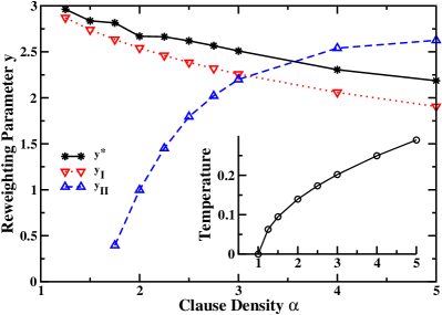
A phase transition occurs for the random Max-$2$-SAT problem at $\alpha=1$, where the mean GSED starts to be positive. The system is then in the spin glass phase at low temperatures for $\alpha>1$. We have determined the spin glass transition temperature $T_{s}(\alpha)$ using the 1RSB mean-field theory Mézard and Parisi (2001); Montanari et al. (2008) (see inset of Fig. 1). At temperature $T=T_{s}(\alpha)$, the equilibrium configuration space divides into exponentially many Gibbs states. The mean GSED is calculated within the 1RSB theory by letting $T=0$ and weighting each Gibbs state by a factor $e^{-yE_{\gamma}^{m}}$, where $E_{\gamma}^{m}$ is the minimum energy of Gibbs state $\gamma$ and the reweighting parameter $y$ is set to a particular value $y=y^{*}$ Mézard and Parisi (2003). At each value of clause density $\alpha$, the 1RSB mean-field theory has two stability thresholds $y_{I}$ and $y_{II}$ Montanari et al. (2004); Mertens et al. (2006); for the mean-field theory to be stable at $y=y^{*}$, it is required that $y_{II}<y^{*}<y_{I}$. As we show in Fig. 1, this condition is violated at $\alpha\geq 1$, suggesting that the GSED obtained by the 1RSB theory is a lower-bound of the true GSED Franz and Leone (2003).

Greedy single-spin flipping for Max-$2$-SAT.—A single-spin flipping process, Gmax, is used to construct low-energy spin configurations for single $2$-SAT formulas. The process starts from a random initial spin configuration $\{\sigma_{i}(0)\}$ at evolution time $t=0$. The evolution time then increases with step $\Delta t=1/N$. A spin configuration $\{\sigma_{i}(t)\}$ at time $t$ is associated with a candidate variable set $C(t)$. A variable belongs to $C(t)$ if and only if reversing its spin does not cause an increase of the configuration energy. A variable $i$ is chosen from the set $C(t)$ uniformly at random, and at evolution time $t^{\prime}=t+\Delta t$, the spin configuration is updated to $\{\sigma_{i}(t^{\prime})\}$ which differs from $\{\sigma_{i}(t)\}$ only at variable $i$. After this spin flipping, the candidate set is also updated to $C(t^{\prime})$.

Figure 2: (Color online) The energy density reached by Gmax as a function of evolution time $t$. The energy trajectory is an averaging over $16$ repeated running of Gmax on a single random $2$-SAT formulas of size $N=10^{6}$ and $\alpha=5.0$. The solid line is the fitting curve of the form $e(t)=e_{0}+h/(\lg t)^{z}$, with parameters $(e_{0},h,z)$ being $(0.433372(8),0.005063(8),1.375(7))$. The asymptotic value $e_{0}$ is very close to the 1RSB lower bound of $0.43273$. Inset shows two segments of a single evolution trajectory.

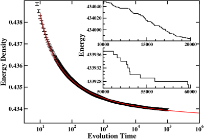
Gmax is a greedy process, the configuration energy never increases with $t$. The density $e(t)$ of energy at time $t$ is $e(t)\equiv E(\sigma_{1}(t),\sigma_{2}(t),\ldots,\sigma_{N}(t))/N$. As an example, Fig. 2 shows the evolution of $e(t)$ for a random $2$-SAT formula with $N=10^{6}$ variables and clause density $\alpha=5.0$. We notice that initially $e(t)$ decreases very fast with $t$. As $t$ increases, the decreasing rate becomes slower and slower and the time interval between two consecutive energy decreases becomes longer and longer (inset of Fig. 2). However, the energy of a single trajectory keeps decreasing even for $t>10^{5}$, suggesting that Gmax is not being trapped by a local energy minimum. The decreasing of $e(t)$ can be well fitted by the following form

$$e(t)=e_{0}+\frac{h}{(\log_{10}t)^{z}}\ ,$$ (2)

with parameters $e_{0}$, $h$, and $z$. The value $e_{0}$ is the asymptotic value of $e(t)$ at $t\rightarrow\infty$, its value is slightly different for different random $2$-SAT instances with the same $N$ and $\alpha$. The fitting parameter $h\sim 10^{-3}$ is much smaller than $e_{0}$, and the scaling exponent $z$ is larger than unity. The observations, (i) $e(t)$ can be expressed as a function of $\log(t)$, and (ii) the asymptotic value $e_{0}$ is very close to the 1RSB lower bound of the mean GSED, suggest that the random Max-$2$-SAT problem has a funnel-shaped energy landscape, to some extent similar to those of protein sequences Onuchic and Wolynes (2004). Gmax visits different funnel-shaped regions when repeated on the same $2$-SAT formula starting from different initial spin configurations, and the bottom energies of these different funnels are very close to each other. However, if Gmax is made to be more greedy, e.g., by preferentially flipping those spins that lead to an energy decrease, the modified dynamics is usually trapped by local minimal regions of the energy landscape.

Figure 3: (Color online) Comparison between the energy density reached by a single run of Gmax on a random $2$-SAT formula of $N=10^{6}$ variables and $\alpha N$ clauses (crosses) and the 1RSB lower bound of mean GSED (solid line). The inset shows the mean energy density reached by a single run of Gmax on $16$ random $2$-SAT formula of fixed clause density $\alpha=5.0$ (diamonds) and $\alpha=10.0$ (squares) and different variable numbers $N$, with the dashed lines marking the corresponding 1RSB lower bounds. The waiting time of Gmax is set to $t=10^{4}$ in all these simulations.

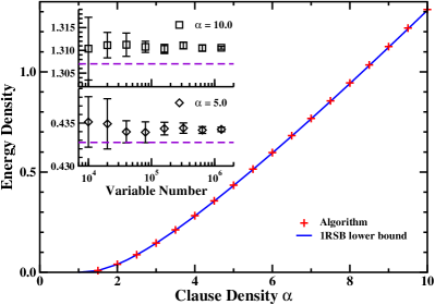
Figure 3 shows the energy density reached by a single run of Gmax at evolution time $t=10^{4}$ on a random $2$-SAT formula of $N=10^{6}$ variables and clause density $\alpha\in[1,10]$. The simulation results are in excellent agreement with the energy density lower bound as obtained by the 1RSB mean-field theory, indicating that Gmax is able to approach the GSED of a large random $2$-SAT formula within a reasonable waiting time. As a stochastic greedy local search process, Gmax is also very fast. We have compared the performance of Gmax with that of the message-passing algorithm SP-y on several large random $2$-SAT problem instances with $N=10^{6}$ and $\alpha=5$ and $\alpha=10$. Gmax is about ten times faster than SP-y and it reaches noticeably lower energy values. The global algorithm SP-y is inspired by the 1RSB spin glass theory Mézard and Montanari (2009); Mézard et al. (2002); Mézard and Zecchina (2002); it contains several adjustable parameters, including the reweighting parameter $y$. As the 1RSB mean-field theory is not sufficient for the random $2$-SAT problem, the message-passing routine of SP-y does not converge. One has to run the non-convergent SP-y process many times with different $y$ values to get good results. The best results obtained by repeated running of SP-y are typically worse than the result of a single run of Gmax.

The inset of Fig. 3 shows the mean energy density value reached by a single run of Gmax at evolution time $t=10^{4}$ on random $2$-SAT formulas of fixed clause density $\alpha$ and different sizes $N$. The reached energy density has only a tiny gap of about $0.002$ above the 1RSB lower bound at $t=10^{4}$, and this gap does not increase with $N$. Such a tiny gap can be further reduced simply by waiting longer.

Gmax for Viana-Bray model.—The $\pm J$ Viana-Bray model on random graphs is equivalent to the random $2$-exclusive-or-satisfiability ($2$-XORSAT) problem, its energy function can be written as

$$E_{2xor}(\sigma_{1},\sigma_{2},\ldots,\sigma_{N})=\sum\limits_{a=1}^{M}\frac{1-J_{a}\sigma_{i}\sigma_{j}}{2}\ .$$ (3)

The coupling constant $J_{a}$ of a clause $a$ takes $\pm 1$ values with equal probability, and the involved two variables $i$ and $j$ of a clause $a$ are chosen from the whole set of $N$ variables uniformly at random. The ground-state energy density of Eq. (3) is positive at clause density $\alpha\equiv M/N>0.5$. For $\alpha>0.5$, the random $2$-XORSAT is in the spin glass phase at low temperatures. A lower bound for the GSED can be obtained using the zero-temperature 1RSB mean-field theory.

Figure 4: (Color online) Comparison between the energy density reached by a single run of Gmax on a random $2$-XORSAT formula of $N=10^{6}$ variables and $\alpha N$ clauses (crosses) and the 1RSB lower bound of mean GSED (solid line). The inset shows the evolution trajectory of a single run of Gmax on a problem instance with $N=10^{6}$ and $\alpha=5.0$.

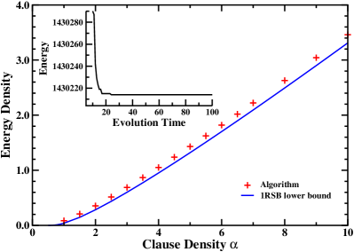
Figure  4 compares the results of a single run of Gmax on a random $2$-XORSAT formula with $N=10^{6}$ variables and $M=\alpha N$ clauses and the energy density 1RSB lower bound. We notice that (see inset of Fig. 4), Gmax quickly comes to a local minimum region of the energy landscape and it is then not able to escape. This is dramatically different from the dynamical behavior observed for the random Max-$2$-SAT problem. There is a noticeable gap between the energy density reached by Gmax and the 1RSB lower-bound.

A $2$-XORSAT constraint $a$ can be expressed in terms of two $2$-SAT constraints: $(1-J_{a}\sigma_{i}\sigma_{j})/2\equiv(1-\sigma_{i})(1+J_{a}\sigma_{j})/4+(1+\sigma_{i})(1-J_{a}\sigma_{j})/4$. These two SAT constraints form a short loop between the two involved variables $i$ and $j$. Therefore, a random $2$-XORSAT formula with clause density $\alpha$ can be converted to a modified random $2$-SAT formula with clause density $2\alpha$. The GSED of the random $2$-XORSAT problem at clause density $\alpha$ is only slightly higher than that of the random $2$-SAT problem at clause density $2\alpha$ (for example, according to the 1RSB mean-field theory, the GSED of random $2$-XORSAT is $1.320$ at $\alpha=5.0$ and that of random $2$-SAT is $1.307$ at $\alpha=10$). The existence of an extensive number of short loops in the modified random $2$-SAT problem therefore does not have much influence on the GSED. However, it changes the system’s energy landscape significantly.

Discussion.—The random Max-$2$-SAT problem is in the spin glass phase at low temperatures. However we found that, for single large Max-$2$-SAT problem instances, a simple greedy single-spin flipping process Gmax is able to reach spin configurations with energy densities extremely close to the lower bound of mean ground-state energy density as predicted by the 1RSB mean-field theory. Such an observation is contrary to the conventional belief that greedy dynamics will be trapped into local stable regions of the energy landscape, whose energy densities are markedly higher than the ground-state value Ricci-Tersenghi (2010). From the logarithmic dependence of the energy density $e(t)$ with the evolution time $t$ [Eq. (2)], we infer that, as the reached energy density is close to the asymptotic value $e_{0}$, the configuration energy is further decreased by accumulating spin local modifications into configuration rearrangements of larger and larger scale Zhou and Wang (2010). This dynamical behavior is consistent with an energy landscape with many rugged and deep funnel-shaped regions. On the other hand, the energy landscape of the Max-$2$-XORSAT problem (the Viana-Bray model) appears to have a very different structure.

Our findings call for understanding from the theoretical side. Gmax is simply a single-spin Glauber dynamics quenched at zero temperature. It is highly desirable to have a theoretical understanding on the empirical observation Eq. (2). At the spin glass transition temperature $T_{s}$, many Gibbs states start to form in the equilibrium configuration space. Suppose they are uniformly sampled, what is their energy depth distribution? And how will this distribution change if the Gibbs states at $T_{s}$ are sampled according to the Boltzmann distribution? The theoretical framework of Zdeborova and Krzakala (2010) may be useful for answering these questions.

For random Max-$K$-SAT problems with $K\geq 3$, our simulation results (not shown) suggest that Gmax is not able to find spin configurations with energy densities extremely close to the 1RSB-predicted ground-state value. However, the gap between the reached energy density and the ground-state energy density is still very small (for example, Gmax reaches an energy density of $0.3315$ at $10^{4}$ evolution steps for a random $3$-SAT formula of $10^{6}$ variables and $\alpha=10$, close to the GSED value of $0.3114$ by 1RSB theory; for a single random $4$-SAT formula of $10^{6}$ variables and $\alpha=20$, these two energy densities are $0.2960$ versus $0.2493$).

This work was partially supported by NSFC Grants 10774150, 10834014, and the 973-Program Grant 2007CB935903. Simulations were performed on the HPC computer cluster of ITP-CAS.

References

- Onuchic and Wolynes (2004) J. N. Onuchic and P. G. Wolynes, Curr. Opin. Struct. Biol. 14, 70 (2004).
- Debenedetti and Stillinger (2001) P. G. Debenedetti and F. H. Stillinger, Nature 410, 259 (2001).
- Kim et al. (2007) S.-Y. Kim, S. J. Lee, and J. Lee, Phys. Rev. B 76, 184412 (2007).
- Carmi et al. (2009) S. Carmi, S. Havlin, C. Song, K. Wang, and H. A. Makse, J. Phys. A: Math. Theor. 42, 105101 (2009).
- Mézard and Montanari (2009) M. Mézard and A. Montanari, Information, Physics, and Computation (Oxford Univ. Press, New York, 2009).
- Dall’Asta et al. (2009) L. Dall’Asta, P. Pin, and A. Ramezanpour, Phys. Rev. E 80, 061136 (2009).
- Mézard et al. (2002) M. Mézard, G. Parisi, and R. Zecchina, Science 297, 812 (2002).
- Mézard and Zecchina (2002) M. Mézard and R. Zecchina, Phys. Rev. E 66, 056126 (2002).
- Achlioptas and Ricci-Tersenghi (2006) D. Achlioptas and F. Ricci-Tersenghi, in Proceedings of the 38th annual ACM symposium on Theory of Computing (Seattle, WA, USA, 2006), pp. 130–139.
- Krzakala et al. (2007) F. Krzakala, A. Montanari, F. Ricci-Tersenghi, G. Semerjian, and L. Zdeborova, Proc. Natl. Acad. Sci. USA 104, 10318 (2007).
- Zhou and Wang (2010) H. Zhou and C. Wang, J. Stat. Mech.: Theor. Exp., P10010 (2010).
- Alava et al. (2008) M. Alava, J. Ardelius, E. Aurell, P. Kaski, S. Krishnamurthy, P. Orponen, and S. Seitz, Proc. Natl. Acad. Sci. USA 105, 15253 (2008).
- Gomes et al. (2008) C. P. Gomes, H. Kautz, A. Sabharwal, and B. Selman, in Handbook of Knowledge Representation, edited by F. van Harmelen, V. Lifschitz, and B. Porter (Elsevier Science, Amsterdam, 2008), chap. 2, pp. 89–134.
- Zdeborova and Krzakala (2010) L. Zdeborova and F. Krzakala, Phys. Rev. B 81, 224205 (2010).
- Mézard and Parisi (2003) M. Mézard and G. Parisi, J. Stat. Phys. 111, 1 (2003).
- Kirkpatrick et al. (1983) S. Kirkpatrick, C. D. Gelatt Jr., and M. P. Vecchi, Science 220, 671 (1983).
- Hukushima and Nemoto (1996) K. Hukushima and K. Nemoto, J. Phys. Soc. Jpn 65, 1604 (1996).
- Boettcher and Percus (2001) S. Boettcher and A. G. Percus, Phys. Rev. Lett. 86, 5211 (2001).
- Lewin et al. (2002) M. Lewin, D. Livnat, and U. Zwick, Lect. Notes Comput. Sci. 2337, 67 (2002).
- Mézard and Parisi (2001) M. Mézard and G. Parisi, Eur. Phys. J. B 20, 217 (2001).
- Montanari et al. (2008) A. Montanari, F. Ricci-Tersenghi, and G. Semerjian, J. Stat. Mech.: Theor. Exper., P04004 (2008).
- Montanari et al. (2004) A. Montanari, G. Parisi, and F. Ricci-Tersenghi, J. Phys. A: Math. Gen. 37, 2073 (2004).
- Mertens et al. (2006) S. Mertens, M. Mézard, and R. Zecchina, Rand. Struct. Algorithms 28, 340 (2006).
- Franz and Leone (2003) S. Franz and M. Leone, J. Stat. Phys. 111, 535 (2003).
- Ricci-Tersenghi (2010) F. Ricci-Tersenghi, Science 230, 1639 (2010).