Extremely Correlated Fermi Liquid Description of Normal State ARPES in Cuprates
Abstract
The normal state single particle spectral function of the high temperature superconducting cuprates, measured by the angle resolved photoelectron spectroscopy (ARPES), has been considered both anomalous and crucial to understand. Here, we report an unprecedented success of the new Extremely Correlated Fermi Liquid theory by Shastry to describe both laser and conventional synchrotron ARPES data (nodal cut at optimal doping) on Bi2Sr2CaCu2O8+δ and synchrotron data on La1.85Sr0.15CuO4. It fits all data sets with the same physical parameter values, satisfies the particle sum rule and successfully addresses two widely discussed “kink” anomalies in the dispersion.
pacs:
71.10.Ay,74.25.Jb,74.72.Gh,79.60.-iAngle resolved photo-electron spectroscopy (ARPES) was the first probe to provide a detailed view of the anomalous nature of high temperature cuprate superconductors, discovering unexpectedly broad spectra with intense and asymmetric tails that have remained an enduring mystery for the last two decades. Conventional data taken with high energy ( eV) photons from synchrotron light sources have recently been supplemented with laser ARPES data Koralek et al. (2006); Zhang et al. (2008) from lower energy (6 or 7 eV) sources. The latter show considerably sharper features near the Fermi energy. A drastic possibility to account for this distinction is that the sudden approximation could break down for the smaller photon energies used in laser ARPES 111In the sudden approximation, the ARPES intensity . Here, is the momentum and is the energy of the final state (as we set in this Letter), where is the number of electrons in the initial state. is the single particle spectral function, is the dipole matrix element, constant for an EDC, and is the Fermi-Dirac function. At the chemical potential .
An important un-answered question is whether the results of the two spectroscopies could be reconciled in a single theoretical framework that does not abandon the sudden approximation. More broadly, can we understand the wide variety of observed lines shapes in a theoretical framework with a sound microscopic basis and a single set of parameters?
In this Letter, we confront a recent theory of Extremely Correlated Fermi Liquids (ECFL) proposed by Shastry Shastry (2011a) with the above challenge. The new formalism is complex and requires considerable further effort to yield numerical results in low dimensions. In the limit of high enough dimensions, however, a remarkably simple expression for the Green’s function emerges; it is significantly different from the standard Fermi Liquid Dyson form, while satisfying the usual sum rules. We use this simple version of ECFL Green’s function in this Letter, motivated by the attractive spectral shapes produced with very few parameters Shastry (2011a). In this Letter we show that already the simplest version of the ECFL theory, with very few parameters, is successful to an unprecedented extent in detailed fitting of a wide variety of normal state cuprate ARPES line shapes. Interesting predictions are made for the higher temperature spectral line skew.
Our focus in this Letter is on the data of optimally doped Bi2Sr2CaCu2O8+δ (Bi2212) and La1.85Sr0.15CuO4 (LSCO) superconductors in the normal state, taken with along the nodal direction connecting to . Most of the data is taken from the published literature, while some original data are also presented (Bi2212 data in Figs. 4,5). Our sample is an optimally doped Bi2212 ( = 91 K), grown by the floating zone method at the Brookhaven National Laboratory (BNL), and was measured at the Stanford Synchrotron Radiation Lightsource (SSRL) beam line 5-4 using 25 eV photons. The resolutions are 15 meV (energy) and 0.3∘ (angle).
Line shape model: The ECFL spectral function is given as a product of an auxiliary Fermi Liquid (aux-FL) spectral function and a second frequency dependent “caparison” factor Shastry (2011a, b):
| (1) |
where is the number of electrons per CuO2 unit cell, , , where is the bare one-electron band dispersion (see later). Here, with
| (2) |
where , is the temperature, and is to be understood as . Here, is the aux-FL energy scale (i.e. high cutoff), and governs the lifetime, and, by causality, the quasi-particle weight (i.e. the wave function renormalization) of the aux-FL, , as identified from 222 where is the Dawson function. and where and are parameters defined in Ref. [Shastry, 2011a]..
The ECFL energy scale measures the “average intrinsic in-elasticity” of the aux-FL. It is given Shastry (2011a) as
| (3) |
where denotes averaging over the first Brillouin zone.
The parameters that enter this description are now listed. The “primary parameters” defining the ECFL fit consist of the dispersion taken from band theory, the density , temperature , and the aux-FL parameters , , , . Of the last four parameters, only two are free parameters. For instance, and can be taken as free parameters, and and can be calculated using the equation for and Eq. 3, respectively.
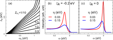
The parameter in Eq. (2) is an additional “secondary parameter” 333By secondary, we mean “intrinsic (i.e. part of ) but dependent on the effective sample quality.” with respect to the ECFL theory Shastry (2011a). Its origin is in impurity scattering as argued in Abrahams and Varma (2000), and additionally, in scattering with surface imperfections. Our fits determine eV for laser ARPES and eV for conventional ARPES. Greater penetration depth in laser ARPES suggests that it should be less sensitive to surface imperfections, thereby yielding a smaller . We therefore propose that this parameter summarizes the effective sample quality in different experiments. The difference in line shapes arising from these values of is demonstrated in Figs. 1(b,c).
Our strategy is to fix a common set of intrinsic parameters for all the materials, and allow to be determined separately for each class of data. The most time consuming part is the calculation of , the results of which are summarized in Fig. 1(a).
In our line shape analysis (1) we first set , corresponding to the optimal doping. (2) Here is taken to be the un-renormalized band dispersion, taken from the literature Markiewicz et al. (2005), and then scaled to fit the observed occupied band width, 1.5 eV, of the Bi2212 ARPES result Meevasana et al. (2007)444Also, a minor -shift of the theory was necessary ( Å) to match the slightly different values reported in different experiments. (3) We choose , to account for the dispersion renormalization due to the high energy kink Graf et al. (2007); Meevasana et al. (2007), which in this theory is caused by the energy scale (cf. Fig. 5). (4) Finally, in all simulations, we include the finite energy resolution effect and the finite angle resolution effect as a combined Gaussian broadening (10 meV FWHM for laser ARPES and 25 meV FWHM for conventional ARPES) in energy 555The minor effect of the finite angular resolution, significant only for the conventional ARPES data, can be modelled well by an energy broadening..
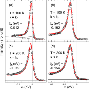
Line shape fit for laser ARPES: Fig. 2 shows the fit of the laser ARPES data with the ECFL line shape. These fits were made using a procedure that is somewhat more restrictive than that in the recent work of Casey and Anderson Casey et al. (2008); Anderson (2006), using the equations of Doniach-Sunjic, Anderson-Yuval, and Nozieres-de Dominicis Doniach and Sunjic (1970); *nozieres_singularities_1969; *yuval_exact_1970 (CADS): we are using global, rather than per-spectrum, fit parameters. However, our fit is somewhat less restricted than other fits shown in this Letter: here we allow a small variation of as in Ref. Casey et al., 2008. We find an excellent fit quality, at least comparable to CADS Casey et al. (2008). The gray line in panel (a) shows our calculation for . Our expectation is that, were the data for available, we would find a reasonable fit in this region as well Koralek (2006), as for other data sets below.
Line shape fit for conventional ARPES: We find that the magnitude of the parameter ( eV) determined from the fit of the sharp laser data works very well also for the conventional ARPES data 666When it is allowed to vary but -independent, it is 0.5 eV within 10 %.. Thus, all parameters other than are fixed, with one small exception in Fig. 4(d), where a slight change in produces a much better fit over a larger energy range for LSCO.
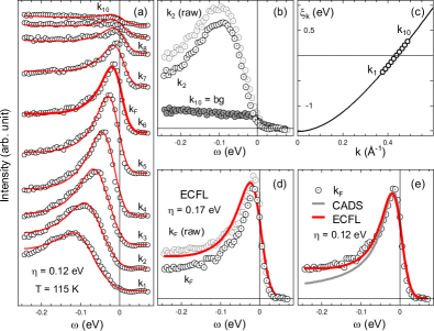
Fig. 3 shows our fit of the data in Ref. Kaminski et al., 2001 with a single free parameter . The amount of the “extrinsic background” (bg) in ARPES is an issue of importance Olson et al. (1990); Gweon et al. (2003); Kaminski et al. (2004), especially when analyzing the conventional ARPES data. Here we fit the bg subtracted data, as well as the raw data (panel d). For subtracting the bg, we use an often-used procedure Kaminski et al. (2004); Valla et al. (1999) of equating the background to a fraction (“bg scaling factor”) of the data far beyond the Fermi surface crossing ( for this data set). The bg scaling factor, 1/2 for this figure, is determined to be the maximum value for which the resulting intensity is not negative. As shown in the panel d, the ECFL fit remains good by adjusting , whether or not the extrinsic background is subtracted. In contrast, we find that the CADS theory, notwithstanding its notable successes Anderson (2008); Casey et al. (2008), cannot cope with even the background subtracted data (Fig. 3e), giving too steep a fall off towards the left. Likewise, the MFL fits Varma et al. (1989); Abrahams and Varma (2000) have been shown to compare well with the data only after substantial background subtraction Valla et al. (1999); Kaminski et al. (2005).
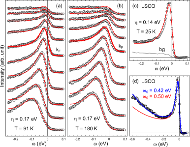
Our own data on Bi2212 data, taken at and well above , covering a similar temperature range as the laser data of Fig. 2, can be fit equally well with the same background subtraction procedure, i.e. with the “bg scaling factor” (1/2), as shown in Fig. 4.
We also find that the data for a lower- cuprate LSCO can be fit very well with the same intrinsic parameters. Here, we shall discuss only the data for brevity. In this case, we determine that the “bg scaling factor” be 1. The subtracted “bg” data Yoshida et al. (2007); Yoshida (2001) is shown as the gray curve in Fig. 4(c). Given their weak superconductivity features Yoshida et al. (2007); Yoshida (2001), these LSCO data are taken to represent the normal state property even if the temperature is slightly lower than . As for the Bi2212 case, the data can be fit well even without the background subtraction, if a somewhat greater value ( eV) is used. It is clear, from Fig. 4(c), that the data at a temperature as low as 25 K can be fit very well with the ECFL line shape. In addition, in working with LSCO line shapes, we noticed a steady and rapid rise in intensity beyond = 0.25 eV, a behavior different from that of Bi2212. We leave the full discussion of this non-universal behavior for future work. However, we find it exceptional that the current theory is able to describe the line shape of LSCO up to very high energy, as shown in Fig. 4(d).
Kinks in the spectra: The two independent energy scales and are determined from our fit as eV and eV. These are natural candidates for the two main dispersion anomalies in the cuprates Graf et al. (2007); Lanzara et al. (2001) as in Fig. 5. Well-defined energy distribution curve (EDC: intensity curve at a fixed value) peaks disappear in a wide energy from eV to 1 eV, as observed experimentally for the high energy kink Graf et al. (2007); Meevasana et al. (2007). As this feature already exists in aux-FL, it cannot be associated with but rather with . The (numerical) dynamical mean field theory Byczuk et al. (2007) can already account for this feature as can the present ECFL (analytical) theory.
Turning to the low energy ARPES kink at meV, Figs. 5(c,d,e) illustrate the observed weak dispersion anomaly in the normal state data (c), reproduced in the ECFL theory (d) but not in the aux-FL theory (e). Here we use a visualization method for momentum distribution curve (MDC: intensity curve at a fixed value), an object discussed primarily for low energy kinks. Thus this feature originates from the scale , it causes an increased asymmetry and the (blue) shift of the peak to high hole energy, when the third term in the caparison factor () of Eq. 1 becomes important. To our knowledge, the ECFL theory is a unique analytical theory that has both these kink features arising from purely electronic (extreme) correlations.
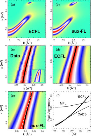
In Fig. 5(f), we show the temperature dependence of the dimensionless peak skew or asymmetry, defined as (HL - HR) / (HL + HR), where HR (HL) is the half-width at half maximum on the right (left) side of the peak. The predicted -dependent asymmetry, predicted even greater for eV (synchrotron data; not shown), would be interesting to explore in the future.
Further work is necessary to refine the picture suggested in this Letter. For example, as increases, the line shape becomes somewhat too asymmetric. Work is also in progress to apply the theory to two particle response as seen, e.g., in optical conductivity. We have checked that the bubble approximation (conductivity as a product of two ’s) shows an agreement in the order of magnitude of the frequency scale and the conductivity.
Conclusions: We have shown that it is possible to understand both ARPES data sets (laser or conventional) comprehensively, with identical physical parameters. Work going beyond the nodal cut and the optimal doping value is in progress. The theory is very tolerant of the uncertainty in the background subtraction for the conventional ARPES data. Additionally, the theory satisfies the global particle sum rule, and contains two inter-dependent energy scales ( and ) that correspond well to the energy scales of the two kinks. Thus the simplest version of the ECFL theory using a small number of parameters, provides a framework to understand the ARPES line shape data for the normal state of the cuprates: it works extremely well across techniques, samples and temperatures.
Portions of this research were carried out at the SSRL, a Directorate of SLAC National Accelerator Laboratory and an Office of Science User Facility operated for the U.S. DOE Office of Science by Stanford University, and at the BNL, supported by the U.S. DOE under Grant No. DE-AC02-98CH10886. The work by GHG was supported partially by COR-FRG at UC Santa Cruz. BSS was supported by U.S. DOE under Grant No. FG02-06ER46319.
References
- Koralek et al. (2006) J. D. Koralek et al., Phys. Rev. Lett. 96, 017005 (2006).
- Zhang et al. (2008) W. Zhang et al., Phys. Rev. Lett. 100, 107002 (2008).
- Note (1) In the sudden approximation, the ARPES intensity . Here, is the momentum and is the energy of the final state (as we set in this Letter), where is the number of electrons in the initial state. is the single particle spectral function, is the dipole matrix element, constant for an EDC, and is the Fermi-Dirac function. At the chemical potential .
- Shastry (2011a) B. S. Shastry, Phys. Rev. Letts. 107, 056403 (2011a).
- Shastry (2011b) B. S. Shastry, arxiv/1104.2633 (2011b).
- Note (2) where is the Dawson function. and where and are parameters defined in Ref. [\rev@citealpshastry_extremely_2011].
- Note (3) By secondary, we mean “intrinsic (i.e.part of ) but dependent on the effective sample quality.”.
- Abrahams and Varma (2000) E. Abrahams and C. M. Varma, Proc. Nat. Acad. Sci. 97, 5714 (2000).
- Markiewicz et al. (2005) R. S. Markiewicz et al., Phys. Rev. B 72, 054519 (2005).
- Meevasana et al. (2007) W. Meevasana et al., Phys. Rev. B 75, 174506 (2007).
- Note (4) Also, a minor -shift of the theory was necessary ( Å) to match the slightly different values reported in different experiments.
- Graf et al. (2007) J. Graf et al., Phys. Rev. Lett. 98, 067004 (2007).
- Note (5) The minor effect of the finite angular resolution, significant only for the conventional ARPES data, can be modelled well by an energy broadening.
- Casey et al. (2008) P. A. Casey et al., Nat Phys 4, 210 (2008).
- Anderson (2006) P. W. Anderson, Nat Phys 2, 626 (2006).
- Doniach and Sunjic (1970) S. Doniach and M. Sunjic, J. Phys. C: Sol. St. Phys. 3, 285 (1970).
- Nozieres and De Dominicis (1969) P. Nozieres and C. T. De Dominicis, Physical Review 178, 1097 (1969).
- Yuval and Anderson (1970) G. Yuval and P. W. Anderson, Phys. Rev. B 1, 1522 (1970).
- Koralek (2006) J. Koralek, Ph.D. thesis, University of Colorado (2006).
- Kaminski et al. (2001) A. Kaminski et al., Phys. Rev. Lett. 86, 1070 (2001).
- Note (6) When it is allowed to vary but -independent, it is 0.5 eV within 10 %.
- Olson et al. (1990) C. G. Olson et al., Phys. Rev. B 42, 381 (1990).
- Gweon et al. (2003) G. Gweon, J. W. Allen, and J. D. Denlinger, Phys. Rev. B 68, 195117 (2003).
- Kaminski et al. (2004) A. Kaminski et al., Phys. Rev. B 69, 212509 (2004).
- Valla et al. (1999) T. Valla et al., Science 285, 2110 (1999).
- Anderson (2008) P. W. Anderson, Phys. Rev. B 78, 174505 (2008).
- Varma et al. (1989) C. M. Varma et al., Phys. Rev. Lett. 63, 1996 (1989).
- Kaminski et al. (2005) A. Kaminski et al., Phys. Rev. B 71, 014517 (2005).
- Yoshida et al. (2007) T. Yoshida et al., J. Phys.: Cond. Matt. 19, 125209 (2007).
- Yoshida (2001) T. Yoshida, Ph.D. thesis, University of Tokyo (2001).
- Lanzara et al. (2001) A. Lanzara et al., Nature 412, 510 (2001).
- Byczuk et al. (2007) K. Byczuk et al., Nat Phys 3, 168 (2007).